Spin dynamics simulations - a powerful method for the study of critical dynamics

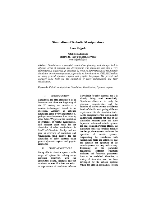
Simulation of Robotic ManipulatorsLeon ŽlajpahJožef Stefan InstituteJamova 39, 1000 Ljubljana, Slovenialeon.zlajpah@ijs.siAbstract: Simulation is a powerful visualization, planning, and strategic tool in different areas of research and development. The simulation has also a very important role in robotics. In the paper we focus on different tools for the dynamic simulation of robot manipulators, especially on those based on MATLAB/Simulink or using general dynamic engines and graphic languages. We present and compare some tools for the simulation of robot manipulators and their visualization.Keywords: Robotic manipulators, Simulation, Visualization, Dynamic enginesI INTRODUCTION Simulation has been recognized as an important tool since the beginning of the 20th century and robotics as a modern technological branch is no exception. Actually, in robotics simulation plays a very important role, perhaps more important than in many other fields. We present the simulationof dynamics of robotic manipulators, and compare some tools for the simulation of robot manipulators in MATLAB/Simulink. Finally and we give an overview of simulation and visualization tools suitable for the simulation of robot systems using general dynamic engines and graphic languages.II SIMULATIONTOOLS Being able to simulate opens a wide range of options for solving many problems creatively. You can investigate, design, visualize, and test an object or even if it does not exists.A large amount of simulation software is available for robot systems, and it is already being used extensively. Simulation allows us to study the structure, characteristics and the function of a robot system at different levels of details each posing different requirements for the simulation tools.As the complexity of the system under investigation increases the role of the simulation becomes more and more important. Advanced robotic systems are quite complex systems. Hence, the simulation tools can certainly enhance the design, development, and even the operation of robotic systems. Augmenting the simulation with visualization tools and interfaces, one can simulate the operation of the robotic systems in a very realistic way. Depending on the particular application different structural attributes and functional parameters have to be modelled. Therefore, a variety of simulation tools has been developed for the robotic systems which are used in mechanical designof robotic manipulators, design of control systems, off-line programmingsystems, to design and test the robotcells, etc. The majority of the robotsimulation tools focus on the motion ofthe robotic manipulator in differentenvironments. As the motionsimulation has a central role in allsimulation systems they all includekinematic or dynamic models of robotmanipulators.The simulation tools for roboticsystems can be divided into two majorgroups: tools based on generalsimulation systems and special toolsfor robot systems.Tools based on general simulationsystems are usually special modules,libraries or user interfaces whichsimplify the building of robot systemsand environments within these generalsimulation systems. One of theadvantages of such integratedtoolboxes is that they enable you touse other tools available in thesimulation system to perform differenttasks. For example, to design controlsystem, to analyse simulation results,to visualize results, etc. The mostpopular general simulation tools whichare used also for simulation of robotsystems are MATLAB/Simulink,Dymola/Modelica, 20-sim, Mathemati-ca, etc.Special simulation tools for robotscover one or more tasks in roboticslike off-line programming, design ofrobot work cells, kinematic anddynamic analysis, mechanical design.They can be specialized for specialtypes of robots like mobile robots,underwater robots, parallelmechanisms, or they are assigned topredefined robot family.2.1 MATLAB-based Tools MATLAB is definitely one of the mostused platforms for the modelling andsimulation of various systems and it isnot surprising that it has been usedintensively for the simulation ofrobotics systems. Among others themain reason for that are its capabilitiesof solving problems with matrixformulations and easy extensibility. Asan extension to MATLAB, SIMU-LINK adds many features for easiersimulation of dynamic systems, e.q.graphical model and the possibility tosimulate in real-time. Among specialtoolboxes that have been developed forMATLAB we have selected forcomparison the following four:(a) Planar Manipulators Toolbox(PMT) [1] is intended for thesimulation of planar manipulators withrevolute joints and is based onLagrangian formulation. PlanarManipulators Toolbox can be used tostudy kinematics and dynamics, todesign control algorithms, for trajecoryplanning. It enables also real timesimulation. Due to its concept it is verygood tool for education. To gain thetransparency, special blocks have beendeveloped to calculate the kinematicand dynamic models. These blocks arethen used to build the desired model.Figure 1 shows the dynamic modelwhere an external force acts on theend-effector. The block dymodallwhich calculates the system vectorsand matrices x, J, ˙J, H, h and g andthen joint accelerations are calculatedusing Lagrangian equation.(b) SD/FAST [2] can be used toperform analysis and design studies onany mechanical system which can bemodelled as a set of rigid bodies inter-Figure 1Dynamic model (PMT)connected by joints, influenced by forces, driven by prescribed motions, and restricted by constraints. Here thedynamic model is calculated using SD/FAST library which is based on the advanced Kane’s formulation.(Order(n) formulation). Then using the SD/FAST compiler the dynamic model is generated. The simulation of thewhole system is based on PMT. The only difference is that a special S-function is used to interface SD/FASTprocedures and Simulink.(c) The Robotics Toolbox (RT) [3] provides many functions that are required in robotics and addresses areas such as kinematics, dynamics, and trajectory generation. RT is useful for simulation as well as for analysing the results from experiments with real robots, and can be a powerful tool for education. RT is based on a general method of representing the kinematics and dynamics of serial-link manipulators by description matrices.The inverse dynamics is calculatedusing the recursive Newton-Euler formulation. Although it was initiallymeant to be used with MATLAB, itcan be used also with Simulink. Figure2 shows the block scheme of thedynamic model using RoboticsToolbox.(d) SimMechanics (SM) [4] extendsSimulink with the tools for modellingFigure 2Dynamic model (RT)and simulating mechanical systems.With SimMechanics, you can model and simulate mechanical systems with a suite of tools to specify bodies andtheir mass properties, their possible motions, kinematic constraints, and coordinate systems, and to initiate andmeasure body motions. To get a dynamic model of a robot manipulator we have first to build the link model,i.e. to connect link masses with joints as it is shown on Figure 3. All linkmodels are then connected together tothe complete model. Figure 3Model of one link (SM) 2.2 Other General Simulation Tools Similar as in MATLAB the robotsystem can be simulated in Dymolaand Modelica, or 20-sim. Here, theMulti-Body libraries provide 3-dimen-sional mechanical components tomodel rigid multibody systems, suchas robots. The robot system is built byconnecting blocks representing parts ofthe robot like link bodies, joints, actuators, etc. Figure 4 shows the simulation of KUKA robot in Modelica [5] and Figure 5 shows the simulation of a parallel robotmanipulator with 20-sim [6].Figure 4Simulation of a robot with ModelicaFigure 5Simulation of a Tripod with 20-sim 3DMechanics Toolbox2.3 Multibody Dynamic Enginess In the last years new simulation tools have been available based on general engines for the simulation of physics environments [8, 9, 2]. These engines provide libraries for simulating the multi-body dynamics, i.e. the physics of motion of an assembly of constrained or restrained bodies. As such they encompass the behaviour of nearly every object and among them are, of course, also robot manipulators. These dynamic engines have beside the dynamics simulation engine also acollision detection engine. The collision engine is given information about the shape of each body and then it figures out which bodies touch each other and passes the resulting contact point information to the user. The user can then take the proper actions. Building the model of a robot is straightforward. First you have to create all bodies and connect them if desired with proper joints. For example, the 3DOF model can be defined using Open Dynamic Engine (ODE) as shown in Figure 6.// create worldcontactgroup.create (0); world.setGravity (9.81,0,0);dWorldSetCFM (world.id(),1e-5); dPlane plane(space,0,0,1,0); // fixed robot basexbody[0].create(world);xbody[0].setPosition(0,0,SIDE/2);box[0].create(space,SIDE,SIDE,SIDE); box[0].setBody(xbody[0]);bjoint = dJointCreateFixed (world,0); dJointAttach (bjoint,xbody[0],0); dJointSetFixed (bjoint); // robot linksfor (i=1; i<=NUM; i++) { xbody[i].create(world);xbody[i].setPosition(0,(i-0.5)*LENG,(i+0.5)*SIDE); m.setBox(1,SIDE,LENG,SIDE); m.adjust(MASS);xbody[i].setMass(&m);box[i].create(space,SIDE,LENG,SIDE); box[i].setBody(xbody[i]); }// robot jointsfor (i=0; i<NUM; i++) { joint[i].create(world);joint[i].attach(xbody[i],xbody[i+1]);joint[i].setAnchor(0,(i)*LENG,(i+1)*SIDE); joint[i].setAxis(0,0,1);}Figure 63R planar manipulator simulated with ODEUnfortunately, most of dynamics engines do not support functionality necessary to include robot models in the control algorithms. Advanced control algorithms including robot models include Jacobian matrices, inertia matrices, gravity forces, etc., and they are not explicitly defined. The user can use some implicit algorithms or other tools to get this parameters. The dynamic simulation of multibody systems becomes very important when introducing robotics into human environments [10, 11, 12], where the success will not depend only on the capabilities of the real robots but also on the simulation of such systems. For example, in applications like virtual prototyping, teleoperation, training, collaborative work, and games, physical models are simulated and interacted with both human usersand robots.Figure 7A force-closure grasp of the mug using the DLRhandFor example, the dynamics engine within a robotic grasping simulator known as GraspIt! [13] computes the motions of a group of connected robot elements, such as an arm and a hand, under the influence of controlled motor forces, joint constraint forces, contact forces and external forces. This allows users to dynamically simulate an entire grasping task, as well as test custom robot control algorithms. Fig. 12 shows how a robot hand can grasp a mug. In this example, all contacts between the fingers and the mug and related forces are analysed.III COMPARISONFor comparison reasons we have simulated only the dynamics, without any task controller. In all four cases it has been very easy to build the robot system. One of the differences is that special toolboxes for robots have predefined more specific functions and blocks as the general toolboxes and the other is the execution time. In Fig. 5 we give the execution time for the dynamic model for all four approaches. First we can see that SD/FAST is significantly faster than other and is increasing more slowly versus the degrees-of freedom than other. Next, Planar Manipulators Toolbox is fast for small number of degrees-of-freedom and the execution time increases fast with the number of degrees-of-freedom. The Robotics Toolbox is relatively fast as long as we use only the inverse dynamics. Otherwise, e.g. for the calculation of the Jacobian matrix, it is significantly slower, because the calculation is based on M-functions.ConclusionWe have presented that the simulationis widely used in robotics Actually, advanced robot systems require sophisticated simulation tools which can model accurately enough the physical world at sufficient speed and allow user interaction. New challengesin the simulation of robotic systems are multi-body dynamics that computes robot and object motionsunder the influence of external forces, fast collision detection and contact determination, realistic visualization of the robot and environment, and haptic interaction. Advanced simulation tools are the foundation for the design of sophisticated robot systems, for the application of robots in complex environments and for the development of new control strategies and algorithms. The simulation being once a tool for the analysis of a robot system and task planning has become an open platform for developing new robot systems. In the end, I believe simulation in robotics has reached a very important role and by using different simulation software, the current and future capabilities of complex robotic systems can besignificantly improved.Figure 8Calculation time of a dynamic model of 3Rplanar robot manipulator References[1]L. Žlajpah: Integrated environ-ment for modelling, simulationand control design for roboticmanipulators. J. of Intelligent.and Robotic Systems, 32(2):219-234, 2001[2]Symblic Dynamics, Inc. SD/FASTUser’s Manual, 1994 [3]P. I. Corke: A Robotics Toolboxfor MATLAB. IEEE Robotics &Automation Magazine, 3(1):24-32, 1996[4]The Mathworks. SimMechanics,User’s Guide, 2005[5]Kazi, G. Merk: Experience withRealSim for Robot Applications.Technical report, KUKA RoboterGmbH, 2002[6]20-sim, Controllab Products,/[7]J. F. Nethery, M. W. Spong:Robotica: a Mathematica packagefor robot analysis. IEEE Robotics& Automation Magazine, 1(1),1994[8]Open Dynamics Engine,/ode.html[9]Newton Game Dynamics,/[10]O. Khatib, O. Brock, K.-S.Chang, F. Conti, D. Ruspini:Human-Centered Robotics andInteractive Haptic Simulation. Int.Journal of Robotic Research,23(2):167-178, 2002[11]A. T. Miller, H. I. Christensen:Implementation of multi-rigid-body dynamics within a roboticgrasping simulator. In Proc. IEEEInt. Conf. on Robotics andAutomation, pages 2262-2268,Taipei, Taiwan, 2003[12]J. Go, B. Browning, M. Veloso:Accurate and flexible simulationfor dynamic, vision-centricrobots. In Proceedings ofInternational Joint Conference onAutonomous Agents and Multi-Agent Systems (AAMAS’04), 2004 [13]A. Miller and P. K. Allen:Graspit!: A versatile simulator forrobotic grasping. IEEE Roboticsand Automation Magazine,11(4):110-122, Dec 2004。

a r X i v :c o n d -m a t /0605703v 2 [c o n d -m a t .m e s -h a l l ] 11 A u g 2006Nuclear Spin Effect in Metallic Spin ValveJ.Danon 1and Yu.V.Nazarov 11Kavli Institute of NanoScience,Delft University of Technology,2628CJ Delft,The Netherlands(Dated:February 6,2008)We study electronic transport through a ferromagnet normal-metal ferromagnet system and we investigate the effect of hyperfine interaction between electrons and nuclei in the normal-metal part.A switching of the magnetization directions of the ferromagnets causes nuclear spins to precess.We show that the effect of this precession on the current through the system is large enough to be observed in experiment.In recent years considerable theoretical and experimen-tal work is aimed at the controlled manipulation of elec-tron spin in nanoscale solid state systems,a field com-monly referred to as spintronics [1].The main moti-vations for this research are applications in conventional computer hardware [2]as well as the futuristic possibility of quantum computation [3],using single electron spins as information carrying units (qubits ).For both purposes,understanding the mechanisms of spin polarization,re-laxation,and dephasing in solid state systems is crucial.The branch of metallic spintronics has quickly evolved after the discovery of the giant magnetoresistance (GMR)in hybrid ferromagnetic normal metal structures [4,5].Theoretical and experimental studies on magnetic mutlilayers have not only revealed interesting physics,but also already led to several applications in magneto-electronic devices.Magnetic recording read heads based on the GMR were first developed some ten years ago [6],but nowadays can be found in nearly all hard disk drives.In the context of quantum computation,semiconduc-tor quantum dots are regarded as promising candidates for storing electron spin based qubits [7].Recent progress in quantum manipulation of single spins [8]has over-come the effects of various spin relaxation processes in these devices.The unavoidable hyperfine interaction be-tween electron and nuclear spin presently attracts much attention.It has been identified as the main source of spin relaxation in high-purity samples at low tempera-tures [9,10]and can even govern the electron transport in double dots [11].At present,hyperfine interaction is seen as the main obstacle to demonstrate quantum com-putation with electron spins in solid state devices.In many other fields,for instance nuclear magnetic res-onance (NMR)experiments,hyperfine interactions play a central role already for decades.The Overhauser ef-fect [12]is a common way to increase the degree of nu-clear polarization in metals enhancing NMR peaks.In semiconductors,optical orientation techniques [13]are used to polarize the nuclear system.In the context of metallic devices,hyperfine interaction has been thought to be too weak to influence charge transport directly,and it has been regarded merely as an extra source of spin re-laxation [1].In this paper,we predict a clearly observable hyper-fine effect on electron transport in a metallic device.Thereby we demonstrate that hyperfine interactions may be important and possibly even dominant also for metal-lic spintronic devices.We consider electronic transport through a ferromagnet normal-metal ferromagnet multi-layer.This so-called spin valve is the basic magnetoelec-tronic device and the core component of all GMR based read heads.By changing the magnetization directions of the two ferromagnetic leads,one alters the total resis-tance of the device as well as the degree and direction of electronic polarization in the normal metal part in the presence of a current.Although the spin and particle transport properties of spin valves are well investigated and understood [14],effects of hyperfine interaction in magnetic multilayers have been hardly studied at all.One may think that these effects are negligible owing to the small value of the hyperfine interaction constant A ≃10−6eV in met-als.We show,however,that electron spins accumulating in the normal metal part can build up a significant po-larization of nuclear spins.The direction of this polar-ization is determined by the magnetizations of the leads.If the magnetizations are suddenly changed,this affects the electronic spin distribution in the normal metal part immediately (at a time scale τe ≃10−11s).The nuclear spin polarization reacts on a much longer time scale and will start to precess slowly around its new equilibrium direction.In this paper we are mainly interested in the feedback of the nuclear polarization on the electronic sys-tem.We show that due to such feedback the precession manifests itself as oscillations in the net current through the device.The amplitude of these oscillations is esti-mated as A/E th .Here E th is the Thouless energy char-acterizing the typical electron dwell time in the valve.The estimation is valid provided this time is shorter than the spin relaxation time τsf ,which sets an upper bound for the effect,Aτsf /¯h .For typical parameters,the rela-tive magnitude of the current oscillations can be of the order 10−4∼10−5,which is clearly large enough to be measured in experiments.We model our system as a small metallic island con-nected to two ferromagnetic leads (Fig.1).We assume the island to be smaller than the spin diffusion length l sf and the time an electron spends in the island much2FNFFIG.1:A schematic picture of the system considered.Asmall metallic island is connected to two large ferromagnetic reservoirs with magnetizations m L and m R .The contacts are charcterized by conductances G L and G R ,which consist of spin-dependent parts G ↑and G ↓,and a mixing conductance G ↑↓.The length of the normal metal part is significantly smaller than the spin diffusion length.smaller than τsf ,which allows us to disregard spin-orbitrelaxation mechanisms in the island.We also assume that the resistance of the junctions by far exceeds the resistance of the island itself.In this case,we can de-scribe the electronic states in the island with a single coordinate-independent distribution function f (E,t ).The two ferromagnetic leads are modeled as large reser-voirs in local equilibrium,with magnetizations in arbi-trary directions m L and m R .Assuming for simplicity T =0,we approximate the electronic distribution func-tion in the leads as f L (R )(E )=θ(µL (R )−E ).The dif-ference in chemical potentials is due to the bias voltage applied eV b =µL −µR .We can disregard temperature provided eV b ≫k B T .In our model,the electron spin polarization is mainly determined by the balance of spin-polarized currents flowing into and out of the ferromagnetic leads.However,a significant correction to this balance comes from hyper-fine coupling between the electron and nuclear spins.The resulting change of the polarization affects the net electric current in the device.So we will first derive an expres-sion for hyperfine induced polarization of electrons and nuclei,and then we combine the result with the known expressions for spin transport through spin valves.The Hamiltonian we use to describe the electronic and nuclear states in the island consists of an electronic part and a part describing the hyperfine interactions,ˆH=ˆH el +ˆH hf ˆH el = kǫk ˆa†k ↑ˆa k ↑+ˆa †k ↓ˆa k ↓ ˆHhf =n A n ˆ S n (t )·ˆΨ†(r n )1dt≈ i¯h2ˆH (t ), ˆH (t ′),ˆa †kαˆakβ ,(2)where the indices αand βnow span a 2×2spin space.We see that the expansion can be completely expressedin the commuting operators ˆ S n and ˆa (†).Using Wick’s theorem,we write the terms with fourand six creation and annihilation operators as products of pairs,which then again can be interpreted as distribu-tion functions f (E,t ).Further,we assume that the elec-trons are distributed homogeneously on the island and approximate A n =A/n 0,A being the hyperfine coupling energy of the material and n 0the density of nuclei with non-zero spin [15].We find up to the second orderd fs ¯h S (t ) × f s (t )−12− fs (t )· S (t )f s (t )+13collinear magnetizations.This yieldsd f s τefs (t )+1τeαR [−f p (t )]+βR m R · f s (t ) m R .(4)Following [14],wedescribeeach spin-active junction withfour conductances,G ↑,G ↓and G ↑↓=(G ↓↑)∗.(If the junction is not spin-active,G ↑=G ↓=G ↑↓=G ↓↑=G ).The electron spin is subject to an effective fieldBe =−1Re(G ↑↓L +G ↑↓R ),and we introduce dimensionless parameters characteriz-ing the spin activity of the junctions αL (R )=G ↑L (R )−G ↓L (R )G ↑L (R )+G ↓L (R )βL (R )=2Re(G ↑↓L (R ))−G ↑L (R )−G ↓L (R )dt=1P L[1−f p (t )]−αRdthf=−νeV bd fs dthf+d fs dt=0.(7)As to nuclear polarization at constant voltage and mage-tization,it is of the order of 1owing to a sort of Over-hauser effect produced by non-equilibrium electrons pass-ing the island.Indeed,it follows from Eq.6that the sta-tionary 2 S= f s /[f p (1−f p )+| f s |2].We see that S and fs are parallel under stationary conditions.This is disappointing since this will not result in any precession.The essential ingredient of our proposal is to change in time the magnetization(s)of the leads.Let us consider the effect of sudden change of the magnetization in one of the leads at t =0.The electrons will find their new distri-bution,characterized by fnew ,on a timescale of τe .As we see from (6),the nuclear spin system will start to precessaround fnew with the frequency estimated.The precess-ing polarization will contribute to the effective field Be , B e → B e +A S (t ) /¯h in (7).This will result in a smallcorrection to fnew , f (1),which is visible in the net cur-rent through the junction,due to its oscillating nature.A simple expression for this correction is obtained in the limit of weakly polarizing junctions (αL,R ,βL,R ≪1),f(1)(t )=Aτe 2τe[P R m R −P L m L ]· f(1)(t ).(9)The time dependence of nuclear polarization is still gov-erned by Eq.6.Combining Eqs 8and 9,we find that the time-dependent current follows the behavior of S(t ) and therefore exhibits oscillations with frequency ωthat are44 6812 3 4τd (τ˜)ξb.a.τd0.060.080.10ω (ω˜)ω-10-5 0 5 10 0 1020I (t )/〈I 〉 × 105t (µs)0.5 1t (s)FIG.2:(a)Numerical calculation of the relative current fluc-tuations as a function of time.For t >20µs the t -axis is compressed.We used the parameters chosen in the text and further we took for both contacts α=0.128,β=0.115and P =0.333.The magnetizations switch at t =0from m L =(0,0,1),m R =(0,0,−1)to m L =(0,1,0),m R =(0,0,−1).(b)The dependence of the relaxation time and the frequency of the fluctuations on the asymmetry ξin the conductances,where ˜τ=¯h n 0/πA 2ν2eV b and ˜ω=AνeV b /¯h n 0.damped at the long time scale τd .The amplitude of these oscillations ∆I in the limit of small αand βreads|∆I |¯h | S old × f new ||P R m ⊥R −P L m ⊥L |,(10)again proportional to A/E th .In this equation Sold refers to the nuclear polarization before switching the magnetizations and m ⊥L (R )is the part of mL (R )perpen-dicular to fnew .This relation makes it straightforward that one needs non-collinear magnetizations to observe any effect.In the same limit,the damping time and precession frequency are given byτd =τhfn 0¯h νeV b ξ+ξ−1+2.(12)where ξ=G L /G R characterizes the asymmetry of the conductance of the contacts.In Fig.2a we plotted a numerical solution for the cur-rent ˜I(t )/ I and in 2b the dependence of ωand τd on the asymmetry in conductance of the contacts.For 2a we made use of equations (6)and (7),and inserted realistic αL,R and βL,R .For the parameters used,the estimate(10)of the amplitude is 4.4×10−5.Eqs (11)and (12)give τd =0.63s and ω=1.0×105Hz,in agreement with the plot.Typical currents through spin valves of these dimensions using a bias voltage of 10mV range be-tween 10and 100mA.Oscillations of the order of 10−5-10−4should be clearly visible in experiment.The un-avoidable shot noise due to the discrete nature of the electrons crossing the junctions will not prevent even an accurate single-shot measurement,since the measure-ment time can be of the order of τd .An estimate using (δI )2≃2eI/τd gives a relative error of 10−8-10−9,at least three orders smaller than the oscillations.So far we have assumed precisely uniform electron dis-tributions.In a realistic situation however,the finite re-sistance of the island results in a voltage drop over theisland,thus causing spatial variation of f 0and fs .Impor-tantly,this gives variations in the precession frequencyω∝A | f s |/¯h .Such variation ∆ωover the length of theisland will contribute to an apparent relaxation of the spin polarization,since precession in different points of the island occurs with a slightly different frequency.This effect adds a term 1/τ∗=∆ωto the damping rate 1/τd .Assuming a simple linear voltage drop over the normal metal part,we find 1/τ∗=(G junc /G isl )ω0,i.e.the ratio of the total conductance of the spin valve and the con-ductance of the metal island times the average oscillation frequency ω0.Although the effect can reduce the appar-ent relaxation time,provided (∆ω)τd ≫1,it will not influence the time-dependent current just after t =0.In conclusion,we have shown how hyperfine-induced nuclear precession in the normal metal part of a spin valve can be made experimentally visible.The precession should give a clear signature in the form of small oscil-lations in the net current through the valve after sudden change of the magnetizations of the leads.We found a coupled set of equations describing the nuclear and elec-tron spin dynamics resulting from a second order pertur-bation expansion in the hyperfine contact Hamiltonian.We presented a numerical solution for the net current and derived an estimate for the amplitude of the oscillations.We found that the relative amplitude of these oscillations is sufficiently big to be observable.The authors acknowledge financial support from FOM and useful discussions with G.E.W.Bauer.[1]I.ˇZuti´c ,J.Fabian,and S.Das Sarma,Rev.Mod.Phys.76,323(2004).[2]S.Parkin,X.Jiang,C.Kaiser,A.Panchula,K.Roche,and M.Samant,Proc.IEEE 91,661(2003).[3]D. D.Awschalom, D.Loss,and N.Samarth,eds.,Semiconductor Spintronics and Quantum Computation (Springer-Verlag,Berlin,2002).[4]M.N.Baibich,J.M.Broto, A.Fert,F.Nguyen VanDau,F.Petroff,P.Eitenne,G.Creuzet,A.Friederich,5and J.Chazelas,Phys.Rev.Lett.61,2472(1988). [5]G.Binasch,P.Gr¨u nberg,F.Saurenbach,and W.Zinn,Phys.Rev.B39,4828(1989).[6]S.Parkin,in Annual Review of Materials Science,editedby B.W.Wessels(Annual Review Inc.,Palo Alto,CA, 1995),vol.25,pp.357–388.[7]D.Loss and D.P.DiVincenzo,Phys.Rev.A57,120(1998).[8]J.R.Petta,A.C.Johnson,J.M.Taylor,ird,A.Yacoby,M.D.Lukin,C.M.Marcus,M.P.Hanson,and A.C.Gossard,Science309,2180(2005).[9]I.A.Merkulov,A.L.Efros,and M.Rosen,Phys.Rev.B65,205309(2002).[10]S.I.Erlingsson,Y.V.Nazarov,and V.I.Fal’ko,Phys.Rev.B64,195306(2001).[11]F.H.L.Koppens,J.A.Folk,J.M.Elzerman,R.Han-son,L.H.Willems van Beveren,I.T.Vink,H.P.Tranitz, W.Wegscheider,L.P.Kouwenhoven,and L.M.K.Van-dersypen,Science309,1346(2005).[12]A.W.Overhauser,Phys.Rev.92,411(1953).[13]F.Meier and B.P.Zakharchenya,eds.,Optical orienta-tion(Elsevier,Amsterdam,1984).[14]A.Brataas,Y.V.Nazarov,and G.E.W.Bauer,Phys.Rev.Lett.84,2481(2000).[15]J.Schliemann,A.Khaetskii,and D.Loss,J.Phys.:Con-dens.Matter15,1809(2003).[16]K.Xia,P.J.Kelly,G.E.W.Bauer,A.Brataas,andI.Turek,Phys.Rev.B65,220401(2002).。

simulation parameters and results -回复Simulation Parameters and ResultsIntroduction:Simulation is the process of creating an artificial model of areal-world system to understand its behavior and predict its outcomes. It has become an essential tool in various fields such as engineering, economics, and social sciences. In this article, we will explore the different parameters involved in simulation and discuss how they affect the results obtained.Step 1: Defining the ProblemThe first step in simulation is to define the problem or thereal-world system that needs to be modeled. This involves understanding the objectives and constraints of the system. For example, in a manufacturing process, the objective could be to optimize production while minimizing costs.Step 2: Identifying the VariablesOnce the problem is defined, the next step is to identify the variables that affect the behavior of the system. These variables can be classified into two categories: input variables and output variables. Input variables are the ones that can be controlled or manipulated, such as production rate, machine speed, or inventory levels. Output variables are the ones that are influenced by the input variables, such as production output, average waiting time, or customer satisfaction.Step 3: Determining the ModelAfter identifying the variables, the next step is to determine the model that represents the system. The model can be a mathematical equation, a set of equations, or a computer program. The model should capture the relationships between the variables and enable the simulation of the system's behavior.Step 4: Specifying the AssumptionsIn simulation, assumptions play a crucial role in simplifying the model and making it manageable. Assumptions are necessary because it is not always possible to consider all the factors thatinfluence the system's behavior. Assumptions can be related to the behavior of the variables, the distribution patterns, or the constraints of the system. It is important to clearly state the assumptions made to avoid any confusion in the interpretation of the results.Step 5: Selecting the Simulation TechniqueThere are different simulation techniques available, depending on the nature of the system being modeled. Some common simulation techniques include discrete-event simulation, system dynamics, and agent-based simulation. The selection of the simulation technique depends on factors such as the complexity of the system, the availability of data, and the objectives of the simulation.Step 6: Setting the ParametersOnce the simulation technique is selected, it is essential to set the parameters that define the system's behavior. These parameters can include the initial conditions, the rules governing the system's dynamics, and the decision-making process. For example, in a supply chain simulation, the parameters could be the lead time,order quantities, and reorder points.Step 7: Running the SimulationAfter setting the parameters, the simulation can be run using appropriate software or programming tools. The simulation generates a sequence of values for the output variables based on the specified values of the input variables. The simulation runs for a specific duration or until a predefined condition is met.Step 8: Analyzing the ResultsOnce the simulation is completed, the results need to be analyzed to gain insights into the system's behavior. The analysis can include statistical measures such as mean, standard deviation, or percentiles. It can also involve visualization techniques such as histograms or line graphs to understand the patterns and trends in the data obtained.Step 9: Validating the ModelValidation is the process of comparing the simulation results withreal-world data or observations to ensure the accuracy of the model. If the simulation results closely match the observed behavior, it can be concluded that the model is valid and can be used to make predictions or test scenarios.Step 10: Sensitivity Analysis and Scenario TestingSensitivity analysis involves studying how changes in the input variables affect the output variables. It helps in understanding the critical factors that influence the system's behavior. Scenario testing involves simulating different scenarios to explore the system's response under various conditions. Both sensitivity analysis and scenario testing help in making informed decisions and improving the system's performance.Conclusion:Simulation is a powerful tool for understanding complex systems and making informed decisions. By carefully defining the problem, identifying variables, determining the model, and setting the parameters, accurate results can be obtained. However, it isimportant to interpret the results with caution and validate the model against real-world data. Simulation provides a valuable platform for experimentation and optimization, ultimately leading to better system design and performance.。

Espoo Feb2004'$BEYOND MOLECULAR DYNAMICSHerman J.C.BerendsenBiophysical Chemistry,University of Groningen,the NetherlandsGroningen Institute for Biosciences and Biotechnology(GBB)CSC,EspooLecture nr4,Thursday,5Februari,2004Molecular dynamics with atomic details is limited to time scales in the order of100ns.Events that are in micro-or millisecond range and beyond,as well as systemsizes beyond100,000particles,call for methods to simplify the system.The key is to reduce the number of degrees of freedom.Thefirst task is to define important degrees of freedom.The’unimportant’degrees of freedom must be averaged-out in such a way that the thermodynamic and long time-scale propertiesare preserved.The reduction of degrees of freedom depends on the problem one wishes to solve.One approach is the use of superatoms,lumping several atoms into one interactionunit.The interactions change into potentials of mean force,and the omitted de-grees of freedom are replaced by noise and friction.On an even coarser scale onemay lump many particles together and describe the behavior in terms of densitiesrather than positions.On a mesoscopic(i.e.,nanometer to micrometer)scale,thefluctuations are still important,but on a macroscopic scale they become negligibleand the Navier-Stokes equations of continuumfluid dynamics emerge.A modern development is to handle the continuum equations with particles(DPD:dissipative particle dynamics).'$ Espoo Feb2004 REDUCED SYSTEM DYNAMICSSeparate relevant d.o.f.rand irrelevant d.o.f.rForce on r :part correlated with positions rpart correlated with velocities˙rrest is’noise’,not correlated with positions or velocities of primed par-ticles.F i(t)=−∂V mf∂r i+F frictioni+F i(t)noiseF frictioni(t)is a function of v j(t−τ).F i(t)noise=R i(t)withR i(t) =0v j(t)R i(t+τ) =0(τ>0)R(t)is characterized by stochastic properties:•probability distribution w(R i)dR i•correlation function R i(t)R j(t+τ)Projection operator technique(Kubo and Mori;Zwanzig)give ele-gant framework to describe relation between friction and noise[Van Kampen in Stochastic Processes in Physics and Chemistry(1981):“This equation is exact but misses the point.The distribution cannot be determined without solving the original equation...”)]'$ Espoo Feb2004 POTENTIAL OF MEAN FORCE-1Requirement:Preserve thermodynamics!Helmholtz free energy A:A=−k B T ln QQ=ce−βV(r)d rDefine a reaction coordinateξ(may be more than one dimension).Sep-arate integration over the reaction coordinate from the integral in Q:Q=cdξd r e−βV(r)δ(ξ(r)−ξ)Define potential of mean force V mf(ξ)asV mf(ξ)=−k B T lncd r e−βV(r)δ(ξ(r)−ξ),so thatQ=e−βV mf(ξ)dξandA=−k B T lne−βV mf(ξ)dξNote that the potential of mean force is an integral over multidimensional hyperspace.It is generally not possible to evaluate such integrals from simulations.As we shall see,it will be possible to evaluate derivatives of V mf from ensemble averages.Therefore we shall be able to compute V mf by integration over multiple simulation results,up to an unknown additive constant.'$ Espoo Feb 2004 POTENTIAL OF MEAN FORCE-2To simplify,look at cartesian coordinates.ξ=r .So r are the impor-tant coordinates,and r are the unimportant coordinates.How can we determine the PMF from simulations?Let us perform a simulation in which r is constrained,while r is freeto move.V mf(r )=−k B T lnce−βV(r ,r )d r∂V mf(r )∂r i =∂V(r ,r )∂r ie−βV(r ,r )d re−βV(r r )d r=∂V(r ,r )∂r i= F c i .Derivative of potential of mean force is the ensemble-averaged constraint force(cartesian).The constraint force follows from the coordinate resetting in constraint dynamics.(This is still true in more complex’reaction coordinates’,but there are small metric tensor corrections)'$ Espoo Feb2004DIFFUSION COEFFICIENTHow to determine the diffusion constant from constrained simulations? Determinefluctuation of constraint force∆F c(t)=F c(t)− F c . Fluctuation-dissipation theorem:∆F c(0)∆F c(t) =k B Tζ(t)ζ= ∞ζ(t)dtD=k B T ζHenceD=(k B T)2∞∆F c(0)∆F c(t) dt'$ Espoo Feb 2004LANGEVIN DYNAMICS-1General form of friction force:approximated by linear response in time,linear in velocities:F fr i(t)=m ij tγij(τ)v j(t−τ)dτThis gives(in cartesian coordinates)the generalized Langevin equation:m i d v idt=−∂V mf∂r i−m ijtγij(τ)v j(t−τ)dτ+R i(t)If a constrained dynamics is carried out with r constant(hence v =0), then the’measured’force on i approximates a representation of R i(t). So one can determine an approximation to the noise correlation functionC R ij(τ)= R i(t)R j(t+τ).(assumption:motion of r that determines R(t)is fast compared to the motion of r )There is a relation between friction and noise.Espoo Feb2004'$ LANGEVIN DYNAMICS-2Relation between friction and noiseAverage total energy should be conserved(averaged over time scale large compared to noise correlation time)•Systematic force is conservative(change in kinetic energy cancelschange in V mf)•Frictional force is dissipative:decreases kinetic energy•Stochastic force has infirst order no effect since v j(t)R i(t+τ) =0.In second order it increases the kinetic energy.The cooling by friction should cancel the heating by noise(fluctuation-dissipation theorem).This leads toR(0)R(t) =k B T mγ(t)'$ Espoo Feb 2004LANGEVIN APPROXIMATIONS(write m iγij=ζij)Generalized Langevinm i˙v i(t)=−∂V mf∂x i−jtζij(τ)v j(t−τ)dτ+R i(t)withR i(0)R j(t) =k B Tζji(t) includes coupling(space)and memory(time). Simple Langevin with hydrodynamic couplingm i˙v i(t)=−∂V mf∂x i−jζij v j(t)+R i(t)withR i(0)R j(t) =2k B Tζjiδ(t) includes coupling(space),but no memory. Simple Langevinm i˙v i(t)=−∂V mf∂x i−ζi v i(t)+R i(t)withR i(0)R j(t) =2k B Tζiδ(t)δij includes neither coupling nor memory.'$ Espoo Feb2004BROWNIAN DYNAMICS-1If systematic force does not change much on the time scale of the ve-locity correlation function,we can average over a time∆t>τc.The average acceleration becomes small and can be neglected(non-inertial dynamics):0≈F i(x)−jζij v j(t)+R iwithR i= t+∆ttR(t )dtR i(0)R j(t) =2k B Tζjiδ(t)Be aware that the average acceleration is not zero if there is a cooperative motion with large massHence v j(t)can be solved from matrix equationζv=F+R(t)Solve in time steps∆tRandom force R i withR i =0R i R j =2k B Tζji∆tR i and R j are correlated random numbers,chosen from bivariate gaus-sian distributions.'$ Espoo Feb2004BROWNIAN DYNAMICS-2Without hydrodynamic coupling:v i=F iζi+r ir i is random number chosen from(gaussian)distribution with variance 2k B T∆t/ζi.x i(t+∆t)=x i(t)+v i∆tVelocity can be eliminated.Write D=k B T/ζ(diffusion constant) yields Brownian dynamicsx(t+∆t)=x(t)+Dk B TF(t)∆t+r(t)r =0r2 =2D∆tF must assumed to be constant during∆t.The longer∆t,the smaller the noise.For slow processes in macroscopic times the noise goes to zero.Espoo Feb2004'$ REDUCED PARTICLE DYNAMICSSuperatom approachLump a number of atoms together into one particle(e.g.10monomersof a homopolymer).Design forcefield for those superatoms including bonding and nonbonding terms.For polymer:•soft harmonic spring between particles,representing Gaussian distri-bution of superatom-distance distributions•harmonic angular term in chain,representing stiffness•Lennard-Jones type interactions between particles•solvent:LJ particleDerive parameters from•experimental data(density,heat of vaporization,solubility,surfacetension,...,•atomic simulations of small system(radius of gyration,end-to-enddistance distribution,radial distribution functions,....Perform normal Molecular Dynamics.Adding friction and noise hasinfluence on dynamics,but is not needed for equilibrium properties. Example:Nielsen et al.,J.Chem.Phys.119(2003)2043.Espoo Feb2004'$DPDWe can also describe the space and time-dependent densities as the im-portant variables(e.g.described on a grid of points),and consider all detailed degrees of freedom as unimportant.This leadsfirst to meso-scopic dynamics(still including noise),and for even coarser averagingto the macroscopic Navier-Stokes equation.The Navier-Stokes equation is normally solved on a grid of points. Dissipative Particle Dynamics attempts to solve the Navier-Stokes equations using an ensemble of special particles.Originally proposed by Hoogerbrugge and Koelman,Europhys.Lett.19 (1992)155.Improved by Espa˜n ol,Warren,Flekkoy,Coveney.See article by Espa˜n ol in SIMU Newsletter Issue4,Chapter III,http://simu.ulb.ac.be/newsletters/N4III.pdf。