多目标遗传算法代码
- 格式:doc
- 大小:81.50 KB
- 文档页数:13

邻域培植多目标遗传算法ncga简介邻域培植多目标遗传算法(NCga)是一种用于解决多目标优化问题的进化算法。
与传统的单目标遗传算法不同,多目标遗传算法旨在寻找一组解,这组解中每个解都是最优解的其中之一,而不是一个单一的最优解。
NCga算法是多目标遗传算法的一种改进版本,它主要解决了传统多目标遗传算法在收敛速度和解的多样性方面的不足。
NCga算法的主要特点包括以下几个方面:1. 遗传算法的基本原理:NCga算法是基于遗传算法的基本原理设计的,包括选择、交叉、变异等基本操作。
遗传算法通过模拟生物进化的过程,不断优化种群中的个体,逐步接近最优解。
2. 邻域培植策略:NCga算法引入了邻域培植策略,通过在当前种群中选择最优解的邻域解来更新种群,以提高种群的多样性和全局搜索能力。
3. 多目标优化:NCga算法可以同时优化多个目标函数,找到一组解,这组解中每个解都是最优解的其中之一。
通过多目标优化,NCga算法可以在不同的目标之间找到平衡,得到更加全面的解集。
4. 收敛速度和解的多样性:NCga算法通过邻域培植策略,可以加速算法的收敛速度,同时保持解的多样性,避免陷入局部最优解。
5. 适用范围:NCga算法适用于各种多目标优化问题,包括工程优化、组合优化、调度问题等。
通过调整算法的参数和优化策略,可以灵活应用于不同的问题领域。
总的来说,邻域培植多目标遗传算法(NCga)是一种有效的多目标优化算法,通过结合遗传算法的基本原理和邻域培植策略,可以有效解决多目标优化问题,具有收敛速度快、解的多样性高的优点,适用于各种多目标优化问题的求解。
NCga算法在实际问题中具有广泛的应用前景,可以帮助优化问题的求解,提高问题的解的质量和效率。

多目标遗传优化算法代码
遗传算法是一种常用的优化算法,它模拟了生物进化的过程,通过种群的进化来寻找最优解。
多目标遗传优化算法是遗传算法的一种扩展,用于解决多目标优化问题。
以下是一个简单的伪代码示例,用于说明多目标遗传优化算法的基本思想:
plaintext.
初始化种群。
计算种群中每个个体的适应度(针对多个目标)。
重复执行以下步骤直到满足终止条件:
选择父代个体。
交叉产生子代个体。
变异子代个体。
计算子代个体的适应度(针对多个目标)。
更新种群。
在实际编写多目标遗传优化算法的代码时,需要根据具体的问
题定义适应度函数、选择算子、交叉算子和变异算子等。
此外,还
需要考虑种群大小、迭代次数、交叉概率、变异概率等参数的设置。
对于具体的实现代码,可以使用Python、Java、C++等编程语
言来编写。
在实际编写代码时,需要根据具体的问题进行适当的调
整和优化,以获得更好的求解效果。
总的来说,多目标遗传优化算法是一种强大的优化工具,可以
用于解决多目标优化问题,但在实际应用中需要根据具体的问题进
行适当的调整和优化。
希望这个简单的伪代码示例能够帮助你理解
多目标遗传优化算法的基本思想。
遗传算法( GA , Genetic Algorithm ) ,也称进化算法。
遗传算法是受达尔文的进化论的启发,借鉴生物进化过程而提出的一种启发式搜索算法。
因此在介绍遗传算法前有必要简单的介绍生物进化知识。
一.进化论知识作为遗传算法生物背景的介绍,下面内容了解即可:种群(Population):生物的进化以群体的形式进行,这样的一个群体称为种群。
个体:组成种群的单个生物。
基因 ( Gene ) :一个遗传因子。
染色体 ( Chromosome ):包含一组的基因。
生存竞争,适者生存:对环境适应度高的、牛B的个体参与繁殖的机会比较多,后代就会越来越多。
适应度低的个体参与繁殖的机会比较少,后代就会越来越少。
遗传与变异:新个体会遗传父母双方各一部分的基因,同时有一定的概率发生基因变异。
简单说来就是:繁殖过程,会发生基因交叉( Crossover ) ,基因突变( Mutation ) ,适应度( Fitness )低的个体会被逐步淘汰,而适应度高的个体会越来越多。
那么经过N代的自然选择后,保存下来的个体都是适应度很高的,其中很可能包含史上产生的适应度最高的那个个体。
二.遗传算法思想借鉴生物进化论,遗传算法将要解决的问题模拟成一个生物进化的过程,通过复制、交叉、突变等操作产生下一代的解,并逐步淘汰掉适应度函数值低的解,增加适应度函数值高的解。
这样进化N代后就很有可能会进化出适应度函数值很高的个体。
举个例子,使用遗传算法解决“0-1背包问题”的思路:0-1背包的解可以编码为一串0-1字符串(0:不取,1:取);首先,随机产生M个0-1字符串,然后评价这些0-1字符串作为0-1背包问题的解的优劣;然后,随机选择一些字符串通过交叉、突变等操作产生下一代的M个字符串,而且较优的解被选中的概率要比较高。
这样经过G代的进化后就可能会产生出0-1背包问题的一个“近似最优解”。
编码:需要将问题的解编码成字符串的形式才能使用遗传算法。
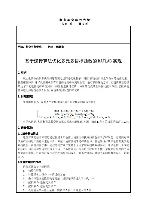
南京航空航天大学共 8 页第 1 页学院:航空宇航学院姓名: 魏德宸基于遗传算法优化多元多目标函数的MATLAB实现0.引言现实生活中的很多决策问题都要考虑同时优化若干个目标,而这些目标之间有时是彼此约束,甚至相互冲突,这样就需要从所有可能的方案中找到最合理、最可靠的解决方案。
而遗传算法是模拟达尔文的遗传选择和自然淘汰的生物进化过程的一种新的迭代的全局优化搜索算法,它能够使群体进化并行搜寻多个目标,并逐渐找到问题的最优解。
1.问题描述变量维数为5,含有2个优化目标的多目标优化问题表达式如下对于该问题,利用权重系数变换法很容易求出最优解,本题中确定f1和f2的权重系数都为0.5。
2.遗传算法2.1遗传算法简述遗传算法的基本原理是通过作用于染色体上的基因寻找好的染色体来求解问题,它需要对算法所产生的每个染色体进行评价,并基于适应度值来选择染色体,使适应性好的染色体有更多的繁殖机会,在遗传算法中,通过随机方式产生若干个所求解问题的数字编码,即染色体,形成初始种群;通过适应度函数给每个个体一个数值评价,淘汰低适应度的个体,选择高适应度的个体参加遗传操作,经过遗产操作后的个体集合形成下一代新的种群,对这个新的种群进行下一轮的进化。
2.2遗传算法的过程遗传算法的基本过程是:1.初始化群体。
2.计算群体上每个个体的适应度值3.由个体适应度值所决定的某个规则选择将进入下一代个体。
4.按概率Pc进行交叉操作。
5.按概率Pm进行变异操作。
6.没有满足某种停止条件,则转第2步,否则进入第7步。
7.输出种群中适应度值最优的染色体作为问题的满意解或最优界。
8.遗传算法过程图如图1:图1 遗传算法过程图3.遗传算法MATLAB代码实现本题中控制参数如下:(1)适应度函数形式FitnV=ranking(ObjV)为基于排序的适应度分配。
(2)交叉概率取为一般情况下的0.7,变异概率取其默认值.(3)个体数目分别为2000和100以用于比较对结果的影响。
多目标多约束优化问题算法多目标多约束优化问题是一类复杂的问题,需要使用特殊设计的算法来解决。
以下是一些常用于解决这类问题的算法:1. 多目标遗传算法(Multi-Objective Genetic Algorithm, MOGA):-原理:使用遗传算法的思想,通过进化的方式寻找最优解。
针对多目标问题,采用Pareto 前沿的概念来评价解的优劣。
-特点:能够同时优化多个目标函数,通过维护一组非支配解来表示可能的最优解。
2. 多目标粒子群优化算法(Multi-Objective Particle Swarm Optimization, MOPSO):-原理:基于群体智能的思想,通过模拟鸟群或鱼群的行为,粒子在解空间中搜索最优解。
-特点:能够在解空间中较好地探索多个目标函数的Pareto 前沿。
3. 多目标差分进化算法(Multi-Objective Differential Evolution, MODE):-原理:差分进化算法的变种,通过引入差分向量来生成新的解,并利用Pareto 前沿来指导搜索过程。
-特点:对于高维、非线性、非凸优化问题有较好的性能。
4. 多目标蚁群算法(Multi-Objective Ant Colony Optimization, MOACO):-原理:基于蚁群算法,模拟蚂蚁在搜索食物时的行为,通过信息素的传递来实现全局搜索和局部搜索。
-特点:在处理多目标问题时,采用Pareto 前沿来评估解的质量。
5. 多目标模拟退火算法(Multi-Objective Simulated Annealing, MOSA):-原理:模拟退火算法的变种,通过模拟金属退火的过程,在解空间中逐渐减小温度来搜索最优解。
-特点:能够在搜索过程中以一定的概率接受比当前解更差的解,避免陷入局部最优解。
这些算法在解决多目标多约束优化问题时具有一定的优势,但选择合适的算法还取决于具体问题的性质和约束条件。
遗传算法多目标优化matlab源代码遗传算法(Genetic Algorithm,GA)是一种基于自然选择和遗传学原理的优化算法。
它通过模拟生物进化过程,利用交叉、变异等操作来搜索问题的最优解。
在多目标优化问题中,GA也可以被应用。
本文将介绍如何使用Matlab实现遗传算法多目标优化,并提供源代码。
一、多目标优化1.1 多目标优化概述在实际问题中,往往存在多个冲突的目标函数需要同时优化。
这就是多目标优化(Multi-Objective Optimization, MOO)问题。
MOO不同于单一目标优化(Single Objective Optimization, SOO),因为在MOO中不存在一个全局最优解,而是存在一系列的Pareto最优解。
Pareto最优解指的是,在不降低任何一个目标函数的情况下,无法找到更好的解决方案。
因此,在MOO中我们需要寻找Pareto前沿(Pareto Front),即所有Pareto最优解组成的集合。
1.2 MOO方法常见的MOO方法有以下几种:(1)加权和法:将每个目标函数乘以一个权重系数,并将其加和作为综合评价指标。
(2)约束法:通过添加约束条件来限制可行域,并在可行域内寻找最优解。
(3)多目标遗传算法:通过模拟生物进化过程,利用交叉、变异等操作来搜索问题的最优解。
1.3 MOO评价指标在MOO中,我们需要使用一些指标来评价算法的性能。
以下是常见的MOO评价指标:(1)Pareto前沿覆盖率:Pareto前沿中被算法找到的解占总解数的比例。
(2)Pareto前沿距离:所有被算法找到的解与真实Pareto前沿之间的平均距离。
(3)收敛性:算法是否能够快速收敛到Pareto前沿。
二、遗传算法2.1 遗传算法概述遗传算法(Genetic Algorithm, GA)是一种基于自然选择和遗传学原理的优化算法。
它通过模拟生物进化过程,利用交叉、变异等操作来搜索问题的最优解。
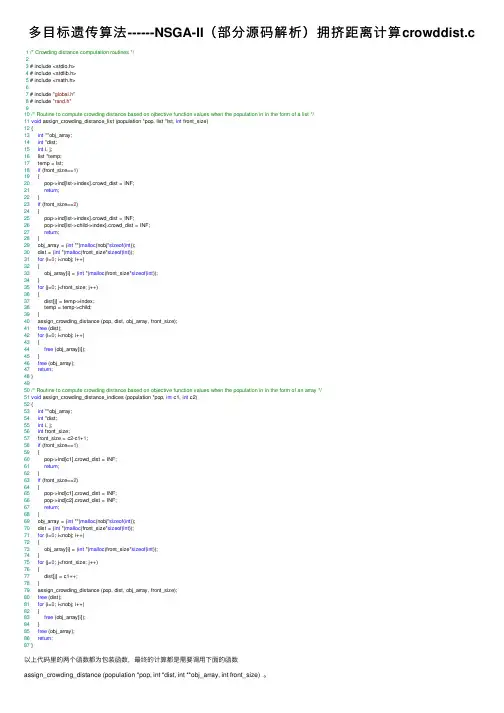
多⽬标遗传算法------NSGA-II(部分源码解析)拥挤距离计算crowddist.c 1/* Crowding distance computation routines */23 # include <stdio.h>4 # include <stdlib.h>5 # include <math.h>67 # include "global.h"8 # include "rand.h"910/* Routine to compute crowding distance based on ojbective function values when the population in in the form of a list */11void assign_crowding_distance_list (population *pop, list *lst, int front_size)12 {13int **obj_array;14int *dist;15int i, j;16 list *temp;17 temp = lst;18if (front_size==1)19 {20 pop->ind[lst->index].crowd_dist = INF;21return;22 }23if (front_size==2)24 {25 pop->ind[lst->index].crowd_dist = INF;26 pop->ind[lst->child->index].crowd_dist = INF;27return;28 }29 obj_array = (int **)malloc(nobj*sizeof(int));30 dist = (int *)malloc(front_size*sizeof(int));31for (i=0; i<nobj; i++)32 {33 obj_array[i] = (int *)malloc(front_size*sizeof(int));34 }35for (j=0; j<front_size; j++)36 {37 dist[j] = temp->index;38 temp = temp->child;39 }40 assign_crowding_distance (pop, dist, obj_array, front_size);41free (dist);42for (i=0; i<nobj; i++)43 {44free (obj_array[i]);45 }46free (obj_array);47return;48 }4950/* Routine to compute crowding distance based on objective function values when the population in in the form of an array */51void assign_crowding_distance_indices (population *pop, int c1, int c2)52 {53int **obj_array;54int *dist;55int i, j;56int front_size;57 front_size = c2-c1+1;58if (front_size==1)59 {60 pop->ind[c1].crowd_dist = INF;61return;62 }63if (front_size==2)64 {65 pop->ind[c1].crowd_dist = INF;66 pop->ind[c2].crowd_dist = INF;67return;68 }69 obj_array = (int **)malloc(nobj*sizeof(int));70 dist = (int *)malloc(front_size*sizeof(int));71for (i=0; i<nobj; i++)72 {73 obj_array[i] = (int *)malloc(front_size*sizeof(int));74 }75for (j=0; j<front_size; j++)76 {77 dist[j] = c1++;78 }79 assign_crowding_distance (pop, dist, obj_array, front_size);80free (dist);81for (i=0; i<nobj; i++)82 {83free (obj_array[i]);84 }85free (obj_array);86return;87 }以上代码⾥的两个函数都为包装函数,最终的计算都是需要调⽤下⾯的函数assign_crowding_distance (population *pop, int *dist, int **obj_array, int front_size) 。
多目标规划有关函数介绍多目标规划(Multi-Objective Programming,MOP)是一种在优化问题中同时优化多个目标函数的数学规划方法。
它与传统的单目标规划(Single-Objective Programming,SOP)方法相比,具有更高的复杂性和难度。
多目标规划的发展可以追溯到20世纪60年代,目前已经成为优化领域的重要研究领域之一、本文将介绍多目标规划中常用的几种函数及其特点。
1. 加权和函数(Weighted Sum Function)加权和函数是多目标规划中最简单和最常用的函数之一、它将多个目标函数按照一定的权重进行加权求和,得到一个综合的目标函数。
加权和函数的数学表示如下:f(x) = ∑(wi * fi(x))其中,f(x)是综合的目标函数,wi是权重系数,fi(x)是第i个目标函数。
加权和函数的特点是容易理解和计算,但存在一个重要的缺点:它偏向于解决具有明确优先级的目标。
因为加权和函数要求设定各个目标函数的权重,而这种权重的设定通常是主观的,因此,加权和函数在处理多目标问题时可能存在一定的偏向性。
2. 目标规则函数(Objective Rule Function)目标规则函数是一种将目标函数转换为约束条件的函数。
它通过将目标函数分别与一组规则进行比较,将满足规则的解视为可行解,进而将优化问题转化为一个带有约束的求解问题。
目标规则函数的数学表示如下:G(x) = (∑(max(0, fi(x) - τi))^2其中,G(x)是目标规则函数,fi(x)是第i个目标函数,τi是规则中的阈值。
目标规则函数的优点是能够帮助用户将优化问题转化为一个有约束的求解问题,从而减少了问题求解的复杂性。
但是,目标规则函数具有确定性和二值化的特性,因此可能会导致信息的丢失和解的不准确。
3. 基因函数(Genetic Function)基因函数是多目标规划中常用的一种函数,它基于遗传算法(Genetic Algorithm,GA),通过模拟自然界中的进化过程,不断演化出较好的解。
遗传算法是一种优化搜索方法,它模拟了自然选择和遗传学中的一些概念,如基因突变、交叉和选择。
这种方法可以用于解决多目标优化问题,其中多个目标之间可能存在冲突。
以下是一个使用C++和OpenCV库实现遗传算法的基本示例。
这个例子解决的是一个简单的多目标优化问题,目标是找到一个最优的图像分割方案,使得两个目标(分割的精度和计算的效率)同时最大化。
注意:这个示例是为了演示遗传算法的基本概念,并不一定适用于所有问题。
你可能需要根据你的具体需求来调整遗传算法的参数和约束条件。
```cpp#include <iostream>#include <vector>#include <algorithm>#include <opencv2/opencv.hpp>// 多目标函数优化struct ObjectiveFunction {std::vector<double> values;void operator()(const std::vector<double>& x) const {// 这里应该根据你的具体问题来定义函数的具体形式// 这里只是一个简单的示例,只考虑了分割精度和计算效率两个目标values.resize(x.size(), 0); // 初始化所有目标值为0values[0] = 1.0; // 精度目标values[1] = 1.0; // 效率目标}};class GeneticAlgorithm {public:GeneticAlgorithm(int populationSize, int generations, double crossoverRate, double mutationRate) : populationSize(populationSize), generations(generations), crossoverRate(crossoverRate), mutationRate(mutationRate) {} std::vector<std::vector<double>> optimize(const std::vector<std::vector<double>>& inputs) {std::vector<std::vector<double>>bestSolution(inputs.size(),std::vector<double>(populationSize, 0)); // 初始化最优解double bestScore = -1; // 初始最佳分数为-1,通常需要先运行一次算法以找到初始最佳分数for (int generation = 0; generation <generations; ++generation) {std::vector<std::vector<double>>population(populationSize,std::vector<double>(populationSize, 0)); // 初始化种群for (int i = 0; i < populationSize; ++i) { std::vector<double>randomSolution(inputs.size(), 0); // 随机生成解for (int j = 0; j < inputs.size(); ++j) {randomSolution[j] = inputs[j][rand() % inputs[j].size()]; // 在输入范围内随机选择一个数作为解}population[i] = randomSolution; // 将随机解加入种群}while (!population.empty()) { // 当种群不为空时继续迭代std::sort(population.begin(), population.end(), [](const std::vector<double>& a, const std::vector<double>& b) { // 对种群进行排序,根据适应度进行排序(这里适应度是解的分数)return ObjectiveFunction()(a) > ObjectiveFunction()(b); // 如果分数更高,则适应度更好,优先选择这个解作为下一代解的一部分});std::vector<double>nextGeneration(population[0]); // 选择当前种群中的第一个解作为下一代解的一部分for (int j = 1; j < populationSize; ++j) { // 对剩余的解进行交叉和变异操作,生成下一代解if (rand() / double(RAND_MAX) < crossoverRate) { // 如果满足交叉条件,则进行交叉操作for (int k = 0; k < inputs.size(); ++k) { // 将两个解的部分基因进行交叉操作,生成新的基因序列nextGeneration[k] = population[j][k]; // 将两个解的部分基因复制到下一代解中if (rand() / double(RAND_MAX) < mutationRate) { // 如果满足变异条件,则对部分基因进行变异操作,增加种群的多样性nextGeneration[k] = nextGeneration[k] * (1 - mutationRate) + population[j][k] * mutationRate; // 对部分基因进行变异操作,增加种群的多样性}}} else { // 如果不满足交叉条件,则直接复制当前解作为下一代解的一部分for (int k = 0; k < inputs.size(); ++k) { // 将当前解的部分基因复制到下一代解中 nextGeneration[k] = population[。
1、遗传算法介绍遗传算法,模拟达尔文进化论的自然选择和遗产学机理的生物进化构成的计算模型,一种不断选择优良个体的算法。
谈到遗传,想想自然界动物遗传是怎么来的,自然主要过程包括染色体的选择,交叉,变异(不明白这个的可以去看看生物学),这些操作后,保证了以后的个基本上是最优的,那么以后再继续这样下去,就可以一直最优了。
2、解决的问题先说说自己要解决的问题吧,遗传算法很有名,自然能解决的问题很多了,在原理上不变的情况下,只要改变模型的应用环境和形式,基本上都可以。
但是遗传算法主要还是解决优化类问题,尤其是那种不能直接解出来的很复杂的问题,而实际情况通常也是这样的。
本部分主要为了了解遗传算法的应用,选择一个复杂的二维函数来进行遗传算法优化,函数显示为y=10*sin(5*x)+7*abs(x-5)+10,这个函数图像为:怎么样,还是有一点复杂的吧,当然你还可以任意假设和编写,只要符合就可以。
那么现在问你要你一下求出最大值你能求出来吗?这类问题如果用遗传算法或者其他优化方法就很简单了,为什么呢?说白了,其实就是计算机太笨了,同时计算速度又超快,举个例子吧,我把x等分成100万份,再一下子都带值进去算,求出对应的100万个y的值,再比较他们的大小,找到最大值不就可以了吗,很笨吧,人算是不可能的,但是计算机可以。
而遗传算法也是很笨的一个个搜索,只不过加了一点什么了,就是人为的给它算的方向和策略,让它有目的的算,这也就是算法了。
3、如何开始?我们知道一个种群中可能只有一个个体吗?不可能吧,肯定很多才对,这样相互结合的机会才多,产生的后代才会多种多样,才会有更好的优良基因,有利于种群的发展。
那么算法也是如此,当然个体多少是个问题,一般来说20-100之间我觉得差不多了。
那么个体究竟是什么呢?在我们这个问题中自然就是x值了。
其他情况下,个体就是所求问题的变量,这里我们假设个体数选100个,也就是开始选100个不同的x值,不明白的话就假设是100个猴子吧。
基于遗传算法的多目标优化算法1、案例背景目前的多目标优化算法有很多,Kalyanmoy Deb的NSGA-II(Nondominated Sorting Genetic Algorithm II,带精英策略的快速非支配排序遗传算法)无疑是其中应用最为广泛也是最为成功的一种。
MATLAB自带的gamultiobj函数所采用的算法,就是基于NSGA-II改进的一种多目标优化算法(a variant of NSGA-II)。
gamultiobj函数的出现,为在MATLAB平台下解决多目标优化问题提供了良好的途径。
gamultiobj函数包含在遗传算法与直接搜索工具箱(Genetic Algorithm and Direct Search Toolbox, GADST)中,这里我们称gamultiobj函数为基于遗传算法的多目标优化函数,相应的算法为基于遗传算法的多目标优化算法。
本案例将以gamultiobj函数为基础,对基于遗传算法的多目标优化算法进行讲解,并详细分析其代码,同时通过一个简单的案例介绍gamultiobj函数的使用。
2、案例目录:第9章基于遗传算法的多目标优化算法9.1 案例背景9.1.1多目标优化及Pareto最优解9.1.2 gamultiobj函数9.2 程序实现9.2.1 gamultiobj组织结构9.2.2 gamultiobj函数中的一些基本概念9.2.3 stepgamultiobj函数分析9.2.3.1 stepgamultiobj函数结构及图形描述9.2.3.2 选择(selectiontournament.m)9.2.3.3 交叉、变异、产生子种群和父子种群合并9.2.3.4 计算序值和拥挤距离(nonDominatedRank.m,distancecrowding.m,trimPopulation.m)9.2.3.5 distanceAndSpread函数9.2.4 gamultiobj函数的调用9.2.4.1 通过GUI方式调用gamultiobj函数9.2.4.2 通过命令行方式调用gamultiobj函数9.3 案例分析9.3.1 模型建立9.3.2 使用gamultiobj函数求解多目标优化问题9.3.3 结果分析9.4 参考文献3、案例实例及结果:作为案例,这里将使用MATLAB自带的基于遗传算法的多目标优化函数gamultiobj求解一个简单的多目标优化问题。
nsga2算法 python代码NSGA-II(Nondominated Sorting Genetic Algorithm II)是一种多目标优化算法,适用于解决具有多个决策变量和目标函数的优化问题。
该算法引入了非支配排序和拥挤度距离的概念,能够在不依赖问题特定知识的情况下高效地搜索多目标优化问题的解集。
在NSGA-II中,算法的核心部分包括:选择、交叉和变异。
首先,通过使用快速非支配排序将种群划分为不同的前沿,并计算每个个体的拥挤度距离。
然后,通过轮盘赌选择方法,选择与给定前沿相同数量的个体作为下一代的父代。
接下来,对选择的父代进行交叉和变异操作产生新的个体,并将其添加到子代中。
最后,通过混合父代和子代的方式生成下一代种群,并重复以上步骤直到满足停止条件。
下面是一个简单的NSGA-II算法的Python实现:```pythonimport random#定义目标函数def obj_func(x):return [x[0]**2, (x[0]-2)**2]#定义个体类class Individual:def __init__(self, x):self.x = xself.obj_values = obj_func(x)self.rank = Noneself.crowding_distance = None#初始化种群def init_population(pop_size, n_var):population = []for _ in range(pop_size):x = [random.uniform(0, 5) for _ in range(n_var)]population.append(Individual(x))return population#计算个体之间的非支配关系def non_dominated_sort(population):fronts = [[]]for ind in population:ind.domination_count = 0ind.dominated_set = []for other_ind in population:if ind.obj_values[0] < other_ind.obj_values[0] and ind.obj_values[1] < other_ind.obj_values[1]:ind.dominated_set.append(other_ind)elif ind.obj_values[0] > other_ind.obj_values[0] and ind.obj_values[1] > other_ind.obj_values[1]:ind.domination_count += 1if ind.domination_count == 0:ind.rank = 0fronts[0].append(ind)curr_front = 0while len(fronts[curr_front]) > 0: next_front = []for ind in fronts[curr_front]:for other_ind in ind.dominated_set: other_ind.domination_count -= 1if other_ind.domination_count == 0: other_ind.rank = curr_front + 1 next_front.append(other_ind)curr_front += 1fronts.append(next_front)return fronts#计算个体的拥挤度距离def crowding_distance_assignment(front):n = len(front)for ind in front:ind.crowding_distance = 0for m in range(len(front[0].obj_values)):front.sort(key=lambda x: x.obj_values[m])front[0].crowding_distance = float('inf')front[n-1].crowding_distance = float('inf')for i in range(1, n-1):front[i].crowding_distance += (front[i+1].obj_values[m] - front[i-1].obj_values[m])#选择操作def selection(fronts, pop_size):new_population = []for front in fronts:crowding_distance_assignment(front)front.sort(key=lambda x: x.crowding_distance, reverse=True)new_population += frontif len(new_population) >= pop_size:breakreturn new_population[:pop_size]#交叉操作def crossover(parent1, parent2):n_var = len(parent1.x)child1 = Individual([0]*n_var)child2 = Individual([0]*n_var)#生成交叉点cxpoint1 = random.randint(0, n_var-1)cxpoint2 = random.randint(0, n_var-1)if cxpoint1 > cxpoint2:cxpoint1, cxpoint2 = cxpoint2, cxpoint1#执行交叉child1.x = parent1.x[:cxpoint1] +parent2.x[cxpoint1:cxpoint2] + parent1.x[cxpoint2:] child2.x = parent2.x[:cxpoint1] +parent1.x[cxpoint1:cxpoint2] + parent2.x[cxpoint2:] return child1, child2#变异操作def mutation(individual):n_var = len(individual.x)mutant = Individual(individual.x[:])#选择变异位点mutation_point = random.randint(0, n_var-1)#执行变异mutant.x[mutation_point] = random.uniform(0, 5) return mutant# NSGA-II算法主函数def nsga2(pop_size, n_var, n_gen):population = init_population(pop_size, n_var) for _ in range(n_gen):fronts = non_dominated_sort(population) population = selection(fronts, pop_size)for i in range(pop_size):if random.random() < 0.9:parent1 = random.choice(population)parent2 = random.choice(population)child1, child2 = crossover(parent1, parent2)population[i] = mutation(child1)else:population[i] = mutation(random.choice(population))return population#测试population = nsga2(100, 1, 100)for ind in population:print(ind.x, ind.obj_values)```该例子实现了一个目标函数为两个二次函数的一维优化问题。
多⽬标遗传算法------NSGA-II(部分源码解析)实数、⼆进制编码的变异操作muta。
遗传算法的变异操作1/* Mutation routines */23 # include <stdio.h>4 # include <stdlib.h>5 # include <math.h>67 # include "global.h"8 # include "rand.h"910/* Function to perform mutation in a population */11void mutation_pop (population *pop)12 {13int i;14for (i=0; i<popsize; i++)15 {16 mutation_ind(&(pop->ind[i]));17 }18return;19 }⼀次进化过程中的变异操作,需要调⽤变异函数 mutation_ind 种群个数popsize 次。
函数包装,判断是实数编码还是⼆进制编码并调⽤不同的变异函数。
1/* Function to perform mutation of an individual */2void mutation_ind (individual *ind)3 {4if (nreal!=0)5 {6 real_mutate_ind(ind);7 }8if (nbin!=0)9 {10 bin_mutate_ind(ind);11 }12return;13 }⼆进制编码的变异操作:每个个体的每个变量的⼆进制编码段的每个⽐特位,以变异概率 pmut_bin 进⾏变异。
(单点变异)1/* Routine for binary mutation of an individual */2void bin_mutate_ind (individual *ind)3 {4int j, k;5double prob;6for (j=0; j<nbin; j++)7 {8for (k=0; k<nbits[j]; k++)9 {10 prob = randomperc();11if (prob <=pmut_bin)12 {13if (ind->gene[j][k] == 0)14 {15 ind->gene[j][k] = 1;16 }17else18 {19 ind->gene[j][k] = 0;20 }21 nbinmut+=1;22 }23 }24 }25return;26 }实数编码情况下的变异操作:(多项式变异)1/* Routine for real polynomial mutation of an individual */2void real_mutate_ind (individual *ind)3 {4int j;5double rnd, delta1, delta2, mut_pow, deltaq;6double delta;7double y, yl, yu, val, xy;8for (j=0; j<nreal; j++)9 {10 rnd = randomperc();11if (rnd <= pmut_real)12 {13 y = ind->xreal[j];14 yl = min_realvar[j];15 yu = max_realvar[j];16 delta1 = (y-yl)/(yu-yl);17 delta2 = (yu-y)/(yu-yl);18 delta = minimum (delta1,delta2);19 rnd = randomperc();20 mut_pow = 1.0/(eta_m+1.0);21if (rnd <= 0.5)22 {23 xy = 1.0-delta1;24 val = 2.0*rnd+(1.0-2.0*rnd)*(pow(xy,(eta_m+1.0)));25 deltaq = pow(val,mut_pow) - 1.0;26 }27else28 {29 xy = 1.0-delta2;30 val = 2.0*(1.0-rnd)+2.0*(rnd-0.5)*(pow(xy,(eta_m+1.0)));31 deltaq = 1.0 - (pow(val,mut_pow));32 }33 y = y + deltaq*(yu-yl);34if (y<yl)35 {36 y = yl;37 }38if (y>yu)39 {40 y = yu;41 }42 ind->xreal[j] = y;43 nrealmut+=1;44 }45 }46return;47 }eta_m 为实数编码的多项式变异的参数,为全局设定。
一、简介Matlab非支配遗传算法(NSGA)是一种用于解决多目标优化问题的进化算法。
它通过模拟自然选择的过程,利用遗传操作来搜索问题的最优解集。
NSGA是一种被广泛应用于工程、经济学、管理和其他领域的优化方法,其代码实现在Matlab中十分方便。
二、NSGA算法原理1. 多目标优化问题多目标优化问题是指在考虑多个竞争性目标的情况下,寻找最优解的问题。
传统的单目标优化问题只考虑一个目标函数的最优解,而多目标优化问题需要找到一个最优解集,以平衡多个目标之间的权衡关系。
NSGA算法通过比较个体之间的非支配关系来维护一个解的集合,以保证最终获得均衡的最优解集。
2. NSGA算法流程NSGA算法通过遗传操作(交叉、变异)和非支配排序来进行多目标优化。
其流程包括以下步骤:- 初始化种裙- 根据非支配排序和拥挤度距离进行选择和繁衍- 进行交叉和变异- 更新种裙- 重复以上步骤直到收敛三、Matlab实现NSGA算法代码在Matlab中实现NSGA算法的代码可以遵循以下步骤:1. 定义优化问题的目标函数和约束条件在Matlab中,可以使用函数句柄来表示目标函数和约束条件,例如:```matlabfunction [y1, y2] = objective(x)y1 = x^2;y2 = (x-2)^2;end```2. 设置算法参数对于NSGA算法,需要设置种裙大小、遗传操作的概率、迭代次数等参数。
```matlabpopsize = 100; 种裙大小nvars = 1; 变量个数maxgen = 100; 迭代次数```3. 调用NSGA算法在Matlab中,可以使用现成的优化工具箱函数来调用NSGA算法进行优化。
```matlaboptions =optimoptions(gamultiobj,'PopulationSize',popsize,'MaxGenerati ons',maxgen);[x,fval] = gamultiobj(objective,nvars,[],[],[],[],[],[],options);```四、NSGA算法在工程领域的应用NSGA算法在工程领域有着广泛的应用,例如在电力系统优化、机械设计、交通规划等方面。
% function nsga_2(pro)%% Main Function% Main program to run the NSGA-II MOEA.% Read the corresponding documentation to learn more about multiobjective% optimization using evolutionary algorithms.% initialize_variables has two arguments; First being the population size% and the second the problem number. '1' corresponds to MOP1 and '2'% corresponds to MOP2.%inp_para_definition=input_parameters_definition;%% Initialize the variables% Declare the variables and initialize their values% pop - population% gen - generations% pro - problem number%clear;clc;tic;pop = 100; % 每一代的种群数gen = 100; % 总共的代数pro = 2; % 问题选择1或者2,见switchswitch procase 1% M is the number of objectives.M = 2;% V is the number of decision variables. In this case it is% difficult to visualize the decision variables space while the% objective space is just two dimensional.V = 6;case 2M = 3;V = 12;case 3 % case 1和case 2 用来对整个算法进行常规验证,作为调试之用;case 3 为本工程所需;M = 2; %(output parameters 个数)V = 8; %(input parameters 个数)K = 10;end% Initialize the populationchromosome = initialize_variables(pop,pro);%% Sort the initialized population% Sort the population using non-domination-sort. This returns two columns% for each individual which are the rank and the crowding distance% corresponding to their position in the front they belong. 真是牛X了。
chromosome = non_domination_sort_mod(chromosome,pro);%% Start the evolution process% The following are performed in each generation% Select the parents% Perfrom crossover and Mutation operator% Perform Selectionfor i = 1 : gen% Select the parents% Parents are selected for reproduction to generate offspring. The% original NSGA-II uses a binary tournament selection based on the% crowded-comparision operator. The arguments are% pool - size of the mating pool. It is common to have this to be half the% population size.% tour - Tournament size. Original NSGA-II uses a binary tournament% selection, but to see the effect of tournament size this is kept% arbitary, to be choosen by the user.pool = round(pop/2);tour = 2;%下面进行二人锦标赛配对,新的群体规模是原来群体的一半parent_chromosome = tournament_selection(chromosome,pool,tour);% Perfrom crossover and Mutation operator% The original NSGA-II algorithm uses Simulated Binary Crossover (SBX) and% Polynomial crossover. Crossover probability pc = 0.9 and mutation% probability is pm = 1/n, where n is the number of decision variables.% Both real-coded GA and binary-coded GA are implemented in the original% algorithm, while in this program only the real-coded GA is considered.% The distribution indeices for crossover and mutation operators as mu = 20% and mum = 20 respectively.mu = 20;mum = 20;% 针对对象是上一步产生的新的个体parent_chromosome%对parent_chromosome 每次操作以较大的概率进行交叉(产生两个新的候选人),或者较小的概率变异(一个新的候选人)操作,这样%就会产生较多的新个体offspring_chromosome = genetic_operator(parent_chromosome,pro,mu,mum);% Intermediate population% Intermediate population is the combined population of parents and% offsprings of the current generation. The population size is almost 1 and% half times the initial population.[main_pop,temp]=size(chromosome);[offspring_pop,temp]=size(offspring_chromosome);intermediate_chromosome(1:main_pop,:)=chromosome;intermediate_chromosome(main_pop+1:main_pop+offspring_pop,1:M+V)=offspring_chromosom e;%intermediate_chromosome=inter_chromo(chromosome,offspring_chromosome,pro);% Non-domination-sort of intermediate population% The intermediate population is sorted again based on non-domination sort% before the replacement operator is performed on the intermediate% population.intermediate_chromosome = ...non_domination_sort_mod(intermediate_chromosome,pro);% Perform Selection% Once the intermediate population is sorted only the best solution is% selected based on it rank and crowding distance. Each front is filled in% ascending order until the addition of population size is reached. The% last front is included in the population based on the individuals with% least crowding distancechromosome = replace_chromosome(intermediate_chromosome,pro,pop);if ~mod(i,10)fprintf('%d\n',i);endend%% Result% Save the result in ASCII text format.save solution.txt chromosome -ASCII%% Visualize% The following is used to visualize the result for the given problem.switch procase 1plot(chromosome(:,V + 1),chromosome(:,V + 2),'y+');title('MOP1 using NSGA-II');xlabel('f(x_1)');ylabel('f(x_2)');case 2plot3(chromosome(:,V + 1),chromosome(:,V + 2),chromosome(:,V + 3),'*');title('MOP2 using NSGA-II');xlabel('f(x_1)');ylabel('f(x_2)');zlabel('f(x_3)');end%disp('run time is:')%toc; %%%%%%%%%%%%%%%%%%%%%%%%%%%%%%%%%%%%%%%%%%%%%%% %%%%%%%function f = initialize_variables(N,problem)% function f = initialize_variables(N,problem)% N - Population size% problem - takes integer values 1 and 2 where,% '1' for MOP1% '2' for MOP2%% This function initializes the population with N individuals and each% individual having M decision variables based on the selected problem.% M = 6 for problem MOP1 and M = 12 for problem MOP2. The objective space% for MOP1 is 2 dimensional while for MOP2 is 3 dimensional.% Both the MOP's has 0 to 1 as its range for all the decision variables.min = 0;max = 1;switch problemcase 1M = 6;K = 8; % k=决策变量(M=6)+目标变量(K-M=2)=8case 2M = 12;K = 15;case 3 % case 1和case 2 用来对整个算法进行常规验证,作为调试之用;case 3 为本工程所需;M = 8; %(input parameters 个数)K = 10;endfor i = 1 : N% Initialize the decision variablesfor j = 1 : Mf(i,j) = rand(1); % i.e f(i,j) = min + (max - min)*rand(1);end% Evaluate the objective functionf(i,M + 1: K) = evaluate_objective(f(i,:),problem);end %%%%%%%%%%%%%%%%%%%%%%%%%%%%%%%%%%%%%%%%%%%%%%% %%%%%%function f = evaluate_objective(x,problem)% Function to evaluate the objective functions for the given input vector% x. x has the decision variablesswitch problemcase 1f = [];%% Objective function onef(1) = 1 - exp(-4*x(1))*(sin(6*pi*x(1)))^6;sum = 0;for i = 2 : 6sum = sum + x(i)/4;end%% Intermediate functiong_x = 1 + 9*(sum)^(0.25);%% Objective function onef(2) = g_x*(1 - ((f(1))/(g_x))^2);case 2f = [];%% Intermediate functiong_x = 0;for i = 3 : 12g_x = g_x + (x(i) - 0.5)^2;end%% Objective function onef(1) = (1 + g_x)*cos(0.5*pi*x(1))*cos(0.5*pi*x(2));%% Objective function twof(2) = (1 + g_x)*cos(0.5*pi*x(1))*sin(0.5*pi*x(2));%% Objective function threef(3) = (1 + g_x)*sin(0.5*pi*x(1));case 3f = [];%% Objective function onef(1) = 0;%% Objective function onef(2) = 0;end %%%%%%%%%%%%%%%%%%%%%%%%%%%%%%%%%%%%%%%%%%%%%%% %%%%%% Non-Donimation Sort %按照目标函数最小了好% This function sort the current popultion based on non-domination. All the% individuals in the first front are given a rank of 1, the second front% individuals are assigned rank 2 and so on. After assigning the rank the% crowding in each front is calculated.function f = non_domination_sort_mod(x,problem)[N,M] = size(x);switch problemcase 1M = 2;V = 6;case 2M = 3;V = 12;case 3 % case 1和case 2 用来对整个算法进行常规验证,作为调试之用;case 3 为本工程所需;M = 2; %(output parameters 个数)V = 8; %(input parameters 个数)K = 10;endfront = 1;% There is nothing to this assignment, used only to manipulate easily in% MATLAB.F(front).f = [];individual = [];for i = 1 : N% Number of individuals that dominate this individual 支配i的解的个数individual(i).n = 0;% Individuals which this individual dominate 被i支配的解individual(i).p = [];for j = 1 : Ndom_less = 0;dom_equal = 0;dom_more = 0;for k = 1 : Mif (x(i,V + k) < x(j,V + k))dom_less = dom_less + 1;elseif (x(i,V + k) == x(j,V + k))dom_equal = dom_equal + 1;elsedom_more = dom_more + 1;endend% 这里只要考虑到求取得是函数的最小值就可以了,此时支配的概念就会变为谁的函数值小,谁去支配别的解%——————————————————————if dom_less == 0 & dom_equal ~= M % 举个例子,其中i=a,b; j= c,d; 如果i 中的a,b全部大于individual(i).n = individual(i).n + 1; % 或者部分大于j中的c,d(但没有小于的情况),则称为i优于j,elseif dom_more == 0 & dom_equal ~= M % 当i优于j的时候,则此时把individual(i)_n加1individual(i).p = [individual(i).p j]; %如果i中的a,b全部小于或者部分小于j中的c,d(但没有大于的情况),则end %则称为j优于i, 则把此时的j放入individual(i)_P中;end %总之,就是说两个目标变量必须全部大于或者全部小于才能对individual有效。