VUMAT基本知识
- 格式:docx
- 大小:162.91 KB
- 文档页数:9
vumat子程序中props里面用到的输入参数【原创版】目录1.Vumat 子程序的概述2.Props 的定义和作用3.Vumat 子程序中 Props 的输入参数详解4.参数的应用示例5.总结正文【1.Vumat 子程序的概述】Vumat 子程序是一款用于计算机视觉和图像处理领域的深度学习模型。
该模型通过使用大量的训练数据,可以有效地对图像进行处理和分析,以完成各种任务,如目标检测、图像分类和语义分割等。
【2.Props 的定义和作用】在 Vumat 子程序中,Props 是指属性,它是一组定义输入数据的参数。
这些参数可以包括图像的大小、颜色空间、数据类型等,以确保输入数据符合模型的要求。
Props 在 Vumat 子程序中起到了至关重要的作用,因为它们可以有效地组织和管理输入数据,从而使模型训练和预测更加高效和准确。
【3.Vumat 子程序中 Props 的输入参数详解】Vumat 子程序中 Props 的输入参数主要包括以下几个方面:(1)图像大小(Image Size):图像大小是指输入图像的宽度和高度。
在 Vumat 子程序中,图像大小通常以像素为单位进行表示。
(2)颜色空间(Color Space):颜色空间是指输入图像所使用的颜色表示方法。
常见的颜色空间有 RGB、HSV 和 LAB 等。
在 Vumat 子程序中,通常使用 RGB 颜色空间进行图像处理。
(3)数据类型(Data Type):数据类型是指输入数据的类型。
在 Vumat 子程序中,输入数据的类型通常为浮点数(float32)或整数(int32)等。
(4)其他参数:除了上述参数之外,Vumat 子程序中还可能涉及到其他一些参数,如归一化方法、数据增强策略等。
这些参数的具体取值取决于模型的结构和训练需求。
【4.参数的应用示例】假设我们要使用 Vumat 子程序训练一个目标检测模型,那么我们需要为该模型设置适当的 Props 输入参数。
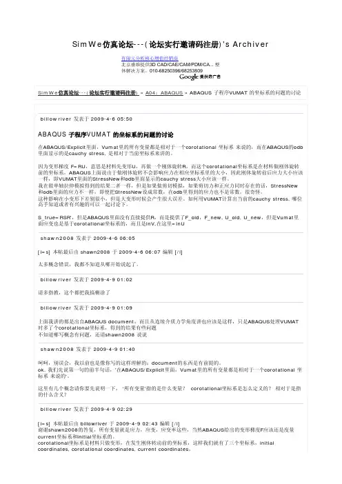
SimWe 仿真论坛---(论坛实行邀请码注册)'s Archiver SimWe 仿真论坛---(论坛实行邀请码注册) » A04:ABAQUS » ABAQUS 子程序VUMAT 的坐标系的问题的讨论billowriver 发表于 2009-4-6 05:50ABAQUS 子程序VUMAT 的坐标系的问题的讨论在ABAQUS/Explicit 里面,Vumat 里的所有变量都是相对于一个corotational 坐标系 来说的,而在ABAQUS 的odb 里面显示的是cauchy stress, 是相对于当前坐标系来讲的。
因为变形梯度 F=RU ,意思是材料先变形U ,再做一个刚体旋转R ,而这个corotational 坐标系是在材料做刚体旋转前的坐标系,ABAQUS 上面说由于做刚体旋转不会影响应力在相应坐标系里的大小,因此刚体旋转前后应力大小应该一样,即VUMAT 里面的StressNew 和odb 里面显示的cauchy stress 大小应该一样。
我在做单轴拉伸模拟得到的结果二者一样,但是如果做剪切模拟,如果剪切力和正应力同时存在的话,StressNew 和odb 里面的应力不一样,即使把StressNew 设成常数,在odb 里得到的应力也不是常数。
很奇怪。
这种影响在小变形下差别很小,但是大变形时候会产生很大误差。
如何用VUMAT 计算出当前的cauchy stress, 哪位高手知道或者有兴趣的可以一起讨论下。
S_true=RSR',但是ABAQUS 里面没有直接提供R ,而是提供了F_old ,F_new, U_old, U_new ,但是Vumat 里面应变也是基于corotational 坐标系的,而且是lnV,在这里=lnUshawn2008 发表于 2009-4-6 06:05[i=s] 本帖最后由 shawn2008 于 2009-4-6 06:07 编辑 [/i]太多概念错误,我都不知道从哪开始说起了。
vulmap 用法Vulmap是一款开源的漏洞扫描框架,用于自动化地扫描和检测Web应用程序的安全漏洞。
它能够帮助安全测试人员和开发人员发现和修复潜在的漏洞,以提高Web应用程序的安全性。
Vulmap的使用方法如下:1.安装及部署:首先,需要在支持PHP的服务器上安装Vulmap。
可以通过克隆Vulmap的GitHub仓库来获取源代码,并将源代码放置在web服务器的根目录下。
然后,通过访问Vulmap的URL来完成Vulmap的部署。
2.目标配置:在Vulmap的管理界面中,可以添加和配置目标,以指定需要扫描的Web应用程序。
目标可以是单个URL或者是URL列表。
配置目标后,可以为目标设置一些扫描参数,如漏洞扫描深度和并发请求数等。
3.漏洞扫描:在目标配置完成后,可以开始进行漏洞扫描。
Vulmap会自动化地进行漏洞检测,并将检测结果以易于阅读的报告形式呈现出来。
扫描过程中会涉及到诸多漏洞检测模块,如SQL注入、XSS、CSRF等。
除了以上基本的使用方法外,可以进一步拓展Vulmap的功能,例如:1.自定义漏洞检测规则:Vulmap提供了一些常见漏洞检测模块,但也可以根据具体需求自定义漏洞检测规则。
通过编写自定义脚本,可以检测特定的漏洞类型或者特定的漏洞细节。
2.集成到CI/CD流程:Vulmap可以与CI/CD工具集成,实现自动化的安全测试。
可以将Vulmap加入到持续集成和持续交付流水线中,定期执行漏洞扫描,并将结果与开发团队共享。
总结来说,Vulmap是一款功能强大的漏洞扫描框架,能够辅助安全测试人员和开发人员快速发现和修复Web应用程序中的安全漏洞。
它的用法包括安装及部署、目标配置、漏洞扫描等。
此外,还可以通过自定义漏洞检测规则和集成到CI/CD流程等方式进行功能拓展。
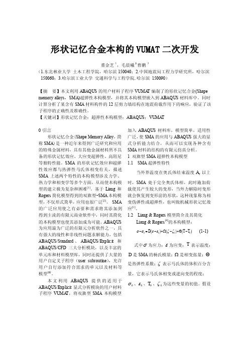
abaqus vumat 原理英文回答:VUMAT is a user-defined material subroutine in Abaqus that allows users to define their own material behavior. It is a powerful tool that can be used to model complex material behavior that cannot be captured by Abaqus' built-in material models.VUMAT is a Fortran subroutine that is called by Abaqus during the solution of a finite element analysis. The subroutine is passed a set of input parameters, including the current stress, strain, and temperature state of the material. The subroutine then calculates the new stress and strain state of the material based on the input parameters and the user-defined material model.VUMAT can be used to model a wide variety of material behaviors, including:Elastic-plastic behavior.Viscoelastic behavior.Damage behavior.Failure behavior.VUMAT is a complex subroutine to write, but it can be a very powerful tool for modeling complex material behavior.中文回答:VUMAT 是 Abaqus 中的一个用户定义材料子程序,允许用户定义自己的材料行为。
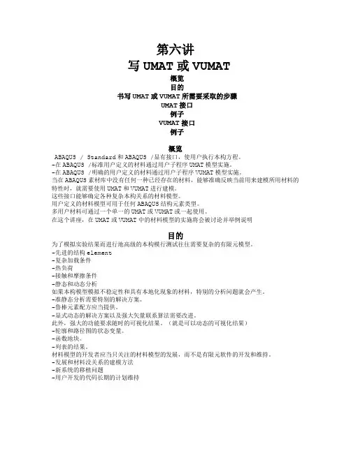
第六讲写UMAT或VUMAT概览目的书写UMAT或VUMAT所需要采取的步骤UMAT接口例子VUMAT接口例子概览ABAQUS / Standard和ABAQUS /显有接口,使用户执行本构方程。
-在ABAQUS /标准用户定义的材料通过用户子程序UMAT模型实施。
-在ABAQUS /明确的用户定义的材料通过用户子程序VUMAT模型实施。
当在ABAQUS素材库中没有任何一种已经存在的材料,能够准确反映当前用来建模所用材料的特性时,就需要使用UMAT和VUMAT进行建模。
这些接口能够确定各种复杂本构关系的材料模型。
用户定义的材料模型可用于任何ABAQUS结构元素类型。
多用户材料可通过一个单一的UMAT或VUMAT或一起使用。
在这个讲座,在UMAT或VUMAT中的材料模型的实施将会被讨论并举例说明目的为了模拟实验结果而进行地高级的本构模行测试往往需要复杂的有限元模型。
-先进的结构element-复杂加载条件-热负荷-接触和摩擦条件-静态和动态分析如果本构模型模拟不稳定性和具有本地化现象的材料,特别的分析问题就会产生。
-准静态分析需要特别的解决方案。
-鲁棒元素配方应当提供。
-显式动态的解决方案以及强大矢量联系算法需要改进。
此外,强大的功能要求随时的可视化结果。
(就是可以动态的可视化结果)-轮廓和路径图的状态变量。
-函数地块。
-列表的结果。
材料模型的开发者应当只关注的材料模型的发展,而不是有限元软件的开发和维持。
-发展和材料没关系的建模方法-新系统的移植问题-用户开发的代码长期的计划维持书写UMAT或VUMAT所需要采取的步骤需要采取的步骤书面UMAT或VUMAT:这就需要定义一个适当的本构方程,如下:-明确定义应力(柯西应力大变形应用)-定义的应力变化率(仅在corotational框架)此外,它很可能需要:-时间,温度,或外地变量这些所依赖东西的定义-内部状态变量的定义,显式的或者用带有偏微分的函数。

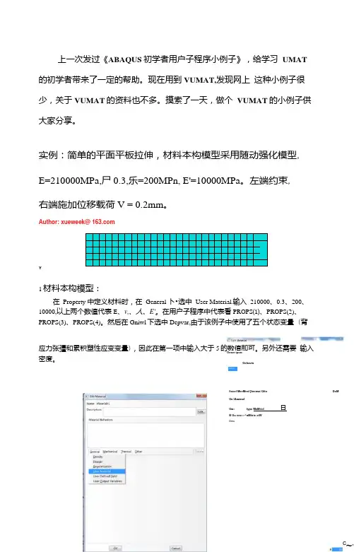
上一次发过《ABAQUS 初学者用户子程序小例子》,给学习 UMAT 的初学者带来了一定的帮助。
现在用到VUMAT,发现网上 这种小例子很少,关于VUMAT 的资料也不多。
摸索了一天,做个 VUMAT 的小例子供大家分享。
实例:简单的平面平板拉伸,材料本构模型采用随动强化模型,E=210000MPa,尸0.3,乐=200MPn, E'=10000MPa 。
左端约束,右端施加位移载荷V = 0.2mm 。
Author: xueweek@ Y1材料本构模型:在 Property 中定义材料时,在 General 卜•选中 User Material.输入 210000、0.3、200、10000,以上两个数值代表E 、v,、人、E'。
在用户子程序中代表看PROPS ⑴、PROPS(2)、 PROPS(3)、PROPS(4)。
然后在Gniwl 下选中Depvar,由于该例子中使用了五个状态变量 (背应力张彊和累积塑性应变变量),因此在第一项中输入大于5的数值即可。
另外还需要 输入密度。
fienel MecMesl [bermai Qtto DcMUs lAawnal Uw«type MxMriol日B Uu vnc»«^nMitric etWDmuOeser ipon: GehavisUse*c ,建模人家都会,故省略2 ABAQUS 中STEP 的设置由于VUMAT 需要用到Explicit 求解,因此需要在step 步骤中设置explicit 选项,如下图, 其设置可以用默认设置。
■ Create Step Name: Step-1Direct cyclic Dynamic, Implicit Dynamic, Explicit Dynamic, Temp-disp, ExplicitGeostatic Heat transfer Mass diffusion SoilsContinue...・:Edit SilWp Mncria^lMst^-al “hzo”Variable rtimber comrollin^ clement dete<<fi Sbg"/t*pi c4o 刃.Njm»cr c< wiv6x dc«xdcrtOxriptio 代Mate^UI Behftticrs*xrd Mzh.rM :dl Rcrmd QtherUm to^otfitu c deptoitnt do3CMNumber H <<Hd “HoBc : DataaoiProcedure type: GeneralInsert new step afterCancel3 ABAQUS调用VUMAT 用户子程序同UMAT用户子程序的调用方法。
vumat子程序中props里面用到的输入参数在Abaqus VUMAT(User Material)子程序中,props是一个参数数组,用于存储材料属性的值。
在VUMAT子程序中,props数组中的值对应于材料定义中的不同材料属性。
以下是props数组中常用的一些输入参数及其含义:
1.props(1):弹性模量(Young's modulus)。
2.props(2):泊松比(Poisson's ratio)。
3.props(3):本构参数(例如,可塑性材料中的流动应力等)。
4.props(4):材料密度。
5.props(5):屈服强度(Yield strength)。
6.props(6):延展性指数/应变硬化参数(strain-hardening
exponent)。
7.props(7):初始硬化参数(initial hardening parameter)。
8.props(8):材料的应变率敏感性(strain rate sensitivity)。
这些参数的具体含义和使用方式可能与你所定义的材料模型相关,不同的材料模型可能需要不同的参数。
因此,在使用VUMAT子程序时,要根据你所使用的材料模型的具体要求和文档进行参数的设置和解释。
此外,其他材料属性也可以在props 数组中定义,具体取决于你所使用的材料模型。
在编写VUMAT子程序时,确保准确理解所使用材料模型的要求和参数定义,以便正确定义和使用props数组中的输入参数。
1. 简介VUMAT子程序是ABAQUS/Standard和ABAQUS/Explicit中提供的用户可编程材料子程序,用于描述复杂的非线性材料行为。
在VUMAT子程序中,props是一组输入参数,用于定义材料的本构关系和其他相关性质。
本文将围绕VUMAT子程序中props所使用到的输入参数展开讨论。
2. 材料本构在VUMAT子程序中,props参数用于定义材料的本构关系。
材料的本构关系描述了材料的应力-应变行为,是模拟材料力学性能的重要组成部分。
props中的输入参数包括弹性模量、泊松比、屈服强度等。
这些参数通过合适的本构模型,可以描述材料在不同应变和应力条件下的响应。
3. 温度相关性质除了力学性质外,props参数还可用于定义材料的温度相关性质。
热膨胀系数、热导率等参数可以通过props输入,从而在材料模拟中考虑温度对材料性能的影响。
这些参数的准确定义对于模拟材料在高温或低温环境下的力学行为非常重要。
4. 动态行为对于需要考虑动态加载条件下材料行为的模拟,props参数也包含了相关的输入项。
材料的惯性系数、动态强度等参数可通过props输入,用于描述材料在高速加载或冲击加载下的响应。
5. 材料失效材料的失效行为也可通过props参数进行定义。
断裂韧性、疲劳强度等参数可以在props中输入,用于描述材料在不同失效机制下的行为。
这些参数对于模拟材料的寿命和可靠性具有重要意义。
6. 参数输入方式在使用VUMAT子程序时,用户需根据所选用的本构模型和材料性质,准确输入props参数。
通常情况下,props参数的输入由用户自行编写的子程序中的对应部分进行设置。
需要注意的是,输入参数的准确性和一致性对于模拟结果的准确性有着重要的影响。
7. 总结在VUMAT子程序中,props参数是用户定义材料本构关系和其他相关性质的重要输入项。
合理准确地设置props参数,对于有效模拟材料的力学行为和失效机制具有重要意义。
一、【子程序】vumat有沙漏问题么?沙漏问题和VUMAT无关,跟你选择的单元有关系,如果你采用减缩积分单元,则会存在沙漏。
有限元的一个核心就是单元模型,其思想是采用单元近似连续体,单元内采用形函数进行插值。
采用全积分的话,可以精确地积出刚度矩阵,但是采用全积分会导致有限元过刚,例如体积锁死和剪切锁死等,因此很多力学及提出了各种各样的单元模型来解决这些问题。
现在用的较多的低阶单元就是一点积分,一点积分的单元由于积分点过少而存在零能模式(沙漏),即在某些变形模式下会出现零应变,这个可以从形函数的公式中推导出来。
所以,沙漏模式是否存在取决你选用的单元,但是你采用ABAQUS的默认设置基本上就可以解决这个问题。
不知道我有没有说清楚二、【基础理论】【概念】剪切锁死、体积锁死、沙漏、零能模式1.剪切锁死(shear locking)简单地说就是在理论上没有剪切变形的单元中发生了剪切变形。
该剪切变形也常称伴生剪切(parasitic shear)。
发生的条件:1.一阶、全积分单元;2.受纯弯状态;产生的结果:使得弯曲变形偏小,即弯曲刚度太刚。
解决方法:1.采用减缩积分;2.细化网格;3.非协调单元;4.假定剪切应变法;2.体积锁死(volumetric locking)简单地说就是应该有单元的体积变化的时候体积却没发生变化。
该原因是受到了伪围压应力(Spurious pressure stresses )。
发生的条件:1.全积分单元;2.材性几乎不可压缩;二阶单元:对于弹塑性材料(塑性部分几乎属于不可压缩),二阶全积分四边形和六面体单元在塑性应变和弹性应变在一个数量级时会发生体积锁死。
二次减缩积分单元发生大应变时体积锁死也伴随出现。
但值得注意的是,一阶全积分单元当采用选择性减缩积分(selectively reduced integration)时可以避免出现体积锁死。
产生的结果:使得体积不变,即体积模量太大,刚度太刚。
NBLOCK: 在调用Vumat时需要用到的材料点的数量Ndir:对称张量中直接应力的数量(sigma11,sigma22,sigma33)Nshr:对称张量中间接应力的数量(sigma12, sigma13, sigma23)Nstatev:与材料类型相关联的用户定义的状态变量的数目Nfieldv:用户定义的外场变量的个数Nprops:用户自定义材料属性的个数Lanneal:指示是否在退火过程中被调用例程的标志。
Lanneal=0,指示在常规力学性能增量,例程被调用。
Lanneal=1表示,这是退火过程,你应该重新初始化内部状态变量,stepTime:步骤开始后的数值totalTime:总时间Dt:时间增量值Cmname:用户自定义的材料名称,左对齐。
它是通过字符串传递的。
一些内部材料模型是以“ABQ_”字符串开头给定的名称。
为了避免冲突,你不应该在“cmname”中使用“ABQ_”作为领先字符串。
coordMp(nblock,*):材料点的坐标值。
它是壳单元的中层面材料点,梁和管(pipe)单元的质心。
charLength(nblock):特征元素长度,是基于几何平均数的默认值或用户子程序VUCHARLENGTH中定义的用户特征元长度。
props(nprops):用户使用的材料属性density(nblock):中层结构的物质点的当前密度strainInc (nblock, ndir+nshr):每个物质点处的应变增量张量relSpinInc (nblock, nshr):在随转系统中定义的每个物质点处增加的相对旋转矢量tempOld(nblock):物质点开始增加时的温度。
defgradOld (nblock,ndir+2*nshr):在增量开始时,每个物质点出的变形梯度张量,在3d中形为(F11, F22,F33,F12,F23,F31,F21,F32,F13),在2d中形为(F11,F22,F33,F12,F21)stretchOld (nblock, ndir+nshr)fieldOld (nblock, nfieldv):在增量开始时,每个物质点处用户定义场变量的值stressOld (nblock, ndir+nshr):在增量开始时,每个物质点处的应力张量:stateOld (nblock, nstatev):在增量开始时,每个物质点处的状态变量:tempNew(nblock):在增量结束时,每个物质点处的温度defgradNew (nblock,ndir+2*nshr):在增量结束时,每个物质点出的变形梯度张量,在3d中形为(F11, F22,F33,F12,F23,F31,F21,F32,F13),在2d中形为(F11,F22,F33,F12,F21)fieldNew (nblock, nfieldv):在增量开始时,每个物质点处用户定义长变量的值Example: Elastic/plastic material with kinematic hardeningAs a simple example of the coding of subroutine VUMAT, consider the generalized plane strain case for an elastic/plastic material with kinematic hardening. The basic assumptions and definitions of the model are as follows.Let be the current value of the stress, and define to be the deviatoric part of the stress. The center of the yield surface in deviatoric stress space is given by the tensor , which has initial values of zero. Thestress difference, , is the stress measured from the center of the yield surface and is given byThe von Mises yield surface is defined aswhere is the uniaxial equivalent yield stress. The von Mises yield surface is a cylinder in deviatoric stress space with a radius ofFor the kinematic hardening model, R is a constant. The normal to the Mises yield surface can be written asWe decompose the strain rate into an elastic and plastic part using an additive decomposition:The plastic part of the strain rate is given by a normality conditionwhere the scalar multiplier must be determined. A scalar measure of equivalent plastic strain rate is defined byThe stress rate is assumed to be purely due to the elastic part of the strain rate and is expressed in terms of Hooke's law bywhere and are the Lamés constants for the material.The evolution law for is given aswhere H is the slope of the uniaxial yield stress versus plastic strain curve.During active plastic loading the stress must remain on the yield surface, so thatThe equivalent plastic strain rate is related to byThe kinematic hardening constitutive model is integrated in a rate form as follows. A trial elastic stress is computed aswhere the subscripts and refer to the beginning and end of the increment, respectively. If the trial stress does not exceed the yieldstress, the new stress is set equal to the trial stress. If the yield stress is exceeded, plasticity occurs in the increment. We then write the incremental analogs of the rate equations aswhereFrom the definition of the normal to the yield surface at the end of the increment, ,This can be expanded using the incremental equations asTaking the tensor product of this equation with , using the yield condition at the end of the increment, and solving for :The value for is used in the incremental equations to determine ,, and .subroutine vumat(C Read only -1 nblock, ndir, nshr, nstatev, nfieldv, nprops, lanneal,2 stepTime, totalTime, dt, cmname, coordMp, charLength,3 props, density, strainInc, relSpinInc,4 tempOld, stretchOld, defgradOld, fieldOld,3 stressOld, stateOld, enerInternOld, enerInelasOld,6 tempNew, stretchNew, defgradNew, fieldNew,C Write only -5 stressNew, stateNew, enerInternNew, enerInelasNew )Cinclude 'vaba_param.inc'CC J2 Mises Plasticity with kinematic hardening for planeC strain case.C Elastic predictor, radial corrector algorithm.CC The state variables are stored as:C STATE(*,1) = back stress component 11C STATE(*,2) = back stress component 22C STATE(*,3) = back stress component 33C STATE(*,4) = back stress component 12C STATE(*,5) = equivalent plastic strainCCC All arrays dimensioned by (*) are not used in this algorithm dimension props(nprops), density(nblock),1 coordMp(nblock,*),2 charLength(*), strainInc(nblock,ndir+nshr),3 relSpinInc(*), tempOld(*),4 stretchOld(*), defgradOld(*),5 fieldOld(*), stressOld(nblock,ndir+nshr),6 stateOld(nblock,nstatev), enerInternOld(nblock),7 enerInelasOld(nblock), tempNew(*),8 stretchNew(*), defgradNew(*), fieldNew(*),9 stressNew(nblock,ndir+nshr), stateNew(nblock,nstatev), 1 enerInternNew(nblock), enerInelasNew(nblock)Ccharacter*80 cmnameCparameter( zero = 0., one = 1., two = 2., three = 3.,1 third = one/three, half = .5, twoThirds = two/three,2 threeHalfs = 1.5 )Ce = props(1)xnu = props(2)yield = props(3)hard = props(4)Ctwomu = e / ( one + xnu )thremu = threeHalfs * twomusixmu = three * twomualamda = twomu * ( e - twomu ) / ( sixmu - two * e )term = one / ( twomu * ( one + hard/thremu ) )con1 = sqrt( twoThirds )Cdo 100 i = 1,nblockCC Trial stresstrace = strainInc(i,1) + strainInc(i,2) + strainInc(i,3) sig1 = stressOld(i,1) + alamda*trace + twomu*strainInc(i,1) sig2 = stressOld(i,2) + alamda*trace + twomu*strainInc(i,2) sig3 = stressOld(i,3) + alamda*trace + twomu*strainInc(i,3) sig4 = stressOld(i,4) + twomu*strainInc(i,4) CC Trial stress measured from the back stresss1 = sig1 - stateOld(i,1)s2 = sig2 - stateOld(i,2)s3 = sig3 - stateOld(i,3)s4 = sig4 - stateOld(i,4)CC Deviatoric part of trial stress measured from the back stresssmean = third * ( s1 + s2 + s3 )ds1 = s1 - smeands2 = s2 - smeands3 = s3 - smeanCC Magnitude of the deviatoric trial stress differencedsmag = sqrt( ds1**2 + ds2**2 + ds3**2 + 2.*s4**2 )CC Check for yield by determining the factor for plasticity,C zero for elastic, one for yieldradius = con1 * yieldfacyld = zeroif( dsmag - radius .ge. zero ) facyld = oneCC Add a protective addition factor to prevent a divide by zeroC when dsmag is zero. If dsmag is zero, we will not have exceededC the yield stress and facyld will be zero.dsmag = dsmag + ( one - facyld )CC Calculated increment in gamma (this explicitly includes theC time step)diff = dsmag - radiusdgamma = facyld * term * diffCC Update equivalent plastic straindeqps = con1 * dgammastateNew(i,5) = stateOld(i,5) + deqpsCC Divide dgamma by dsmag so that the deviatoric stresses areC explicitly converted to tensors of unit magnitude in theC following calculationsdgamma = dgamma / dsmagCC Update back stressfactor = hard * dgamma * twoThirdsstateNew(i,1) = stateOld(i,1) + factor * ds1stateNew(i,2) = stateOld(i,2) + factor * ds2stateNew(i,3) = stateOld(i,3) + factor * ds3stateNew(i,4) = stateOld(i,4) + factor * s4CC Update the stressfactor = twomu * dgammastressNew(i,1) = sig1 - factor * ds1stressNew(i,2) = sig2 - factor * ds2stressNew(i,3) = sig3 - factor * ds3stressNew(i,4) = sig4 - factor * s4CC Update the specific internal energy -stressPower = half * (1 ( stressOld(i,1)+stressNew(i,1) )*strainInc(i,1)1 + ( stressOld(i,2)+stressNew(i,2) )*strainInc(i,2) 1 + ( stressOld(i,3)+stressNew(i,3) )*strainInc(i,3) 1 + two*( stressOld(i,4)+stressNew(i,4) )*strainInc(i,4) ) CenerInternNew(i) = enerInternOld(i)1 + stressPower / density(i)CC Update the dissipated inelastic specific energy -plasticWorkInc = dgamma * half * (1 ( stressOld(i,1)+stressNew(i,1) )*ds11 + ( stressOld(i,2)+stressNew(i,2) )*ds2 1 + ( stressOld(i,3)+stressNew(i,3) )*ds3 1 + two*( stressOld(i,4)+stressNew(i,4) )*s4 ) enerInelasNew(i) = enerInelasOld(i)1 + plasticWorkInc / density(i)100 continueCreturnend。