
levelset_tutorial
- 格式:ppt
- 大小:4.25 MB
- 文档页数:92


Junior High English Tutorial Plan and StrategiesIntroduction:Junior high is a crucial phase for English language learning, as students transition from basic to more complex grammatical structures and vocabulary. An effective tutorial plan with specific measures is necessary to support students in this critical stage.Tutorial Plan:Assessment: Begin with an assessment to identify students' current English proficiency level, strengths, and areas of improvement.Goal Setting: Based on the assessment, set clear and achievable learning goals for the tutorial sessions.Curriculum Outline: Develop a curriculum outline that covers key language areas such as vocabulary, grammar, reading comprehension, and writing skills.Regular Sessions: Schedule regular tutorial sessions, ensuring consistency and frequency for effective learning.Interactive Activities: Incorporate interactive activities and games to engage students and make learning fun.Feedback and Adjustment: Provide regular feedback to students, addressing their performance and areas of improvement. Adjust the tutorial plan accordingly to ensure optimal learning outcomes.Measures:Monitoring Progress: Use standardized tests, quizzes, and assignments to monitor students' progress and adjust the tutorial plan as needed.Encourage Practice: Encourage students to practice English outside of tutorial sessions, such as through reading, watching English movies, or participating in English clubs.Collaborative Learning: Promote collaborative learning among students, encouraging them to work together on assignments and share learning resources.Parental Engagement: Involve parents in the learning process, providing updates on students' progress and seeking their support and feedback.Conclusion:A structured junior high English tutorial plan with targeted measures can significantly enhance students' language skills and confidence. It is important to tailor the plan to each student's needs, fostering a positive and effective learning environment.引言:初中阶段是英语学习的关键时期,学生需要掌握更复杂的语法结构和词汇。

level set 函数Level Set 函数是一种常用的数学工具,用于描述和处理曲线、曲面或其他几何对象的演化和变形。
它在计算机图形学、计算流体力学、图像处理等领域有着广泛的应用。
本文将从Level Set 函数的定义、性质以及应用等方面展开论述。
一、定义Level Set 函数是一种定义在n维欧氏空间中的标量函数,其值表示点到曲线、曲面或其他几何对象的距离。
它的本质是将几何对象的边界定义为函数等值线(level set)所在的位置。
形式化地,对于二维情况,可表示为:Φ(x, y) = 0其中(x, y)为欧氏空间中的点,Φ(x, y)为Level Set 函数。
二、性质Level Set 函数具有以下几个重要性质:1. 常值性:在曲线、曲面或其他几何对象外部,Level Set 函数的值为正数;在几何对象内部,Level Set 函数的值为负数。
2. 平移不变性:Level Set 函数在平移变换下保持不变,即在欧氏空间中平移几何对象不会改变Level Set 函数的形态。
3. 数值梯度:Level Set 函数的梯度是指向几何对象内部的法向量,因此可以通过计算梯度来推断几何对象的演化方向。
4. 光滑性:Level Set 函数可以通过插值或拟合等方法实现光滑化,使得几何对象的演化更加稳定和精确。
三、应用Level Set 函数在各种领域有着广泛的应用,下面列举几个常见的应用场景:1. 计算机图形学:Level Set 函数可以用于实现曲线和曲面的变形和演化,广泛应用于计算机动画、虚拟现实等领域。
2. 计算流体力学:Level Set 函数可以用于模拟流体的自由表面,通过数值计算几何对象的演化,从而实现流体的模拟和分析。
3. 图像处理:Level Set 函数可以用于图像分割、图像修复等任务,通过将图像的边界定义为Level Set 函数等值线的位置,实现对图像的自动分割和修复。
4. 形状优化:Level Set 函数可用于形状优化问题,通过数值计算几何对象的演化,寻找最优形状或最小曲率曲面。
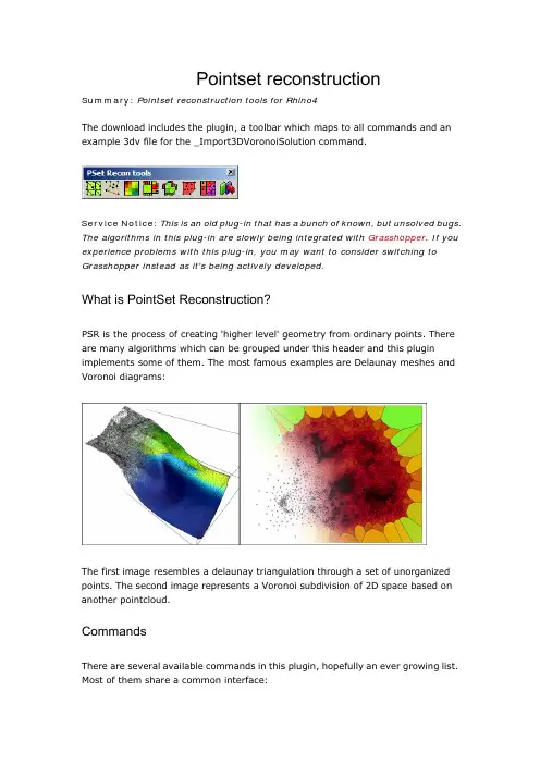
Pointset reconstructionSummary:Pointset reconstruction tools for Rhino4The download includes the plugin, a toolbar which maps to all commands and an example 3dv file for the _Import3DVoronoiSolution command.Service Notice:This is an old plug-in that has a bunch of known, but unsolved bugs. The algorithms in this plug-in are slowly being integrated with Grasshopper. If you experience problems with this plug-in, you may want to consider switching to Grasshopper instead as it's being actively developed.What is PointSet Reconstruction?PSR is the process of creating 'higher level' geometry from ordinary points. There are many algorithms which can be grouped under this header and this plugin implements some of them. The most famous examples are Delaunay meshes and Voronoi diagrams:The first image resembles a delaunay triangulation through a set of unorganized points. The second image represents a Voronoi subdivision of 2D space based on another pointcloud.CommandsThere are several available commands in this plugin, hopefully an ever growing list. Most of them share a common interface:1. Select input geometry2. Change options3. Insert solutionYou can select any amount of Points, Pointclouds,Curves or Meshes as input geometry. If you selectcurves you will be prompted for a division valuewhich will be used to sample the curves. Curves arealso always sampled at their kinks. After you haveselected the input curves, the command will eithercomplete if it has no options or it will draw a previewof the result while providing you with clickablecommand line options. Some options will cause thesolution to become invalid in which case it will haveto be recomputed. This is potentially a veryexpensive operation but you can always abort theseprocesses by pressing the escape key.The available commands are:•Delaunay(wikipedia)•Voronoi(wikipedia)•3DVoronoi(wikipedia)•PixelGrid•OcTree(wikipedia)•QuadTree(wikipedia)•Network(wikipedia)•ConvexHull(wikipedia) ^▪^•SpanningCircle(wikipedia) ^▪^DelaunayDelaunay triangulation is a 2.5Dimensional process of fitting triangles through unorganized points so that there are no gaps left in a mesh. It is well suited for recreating surfaces that are implied by a collection of points. The output is always a mesh (not a NURBs surface) and it cannot deal with z-based overlap of points. The mesh can be coloured using several different shader algorithms (see below). These colours will persist after the mesh is inserted.•Terrain » Apply standard colours which are associated with terrain. You have to specify the water-level and whether or not the terrain is lit from a certain direction as opposed to ambient lighting.•Slope » The steepest areas are coloured green and the flattest areas become yellow. The gradient is scaled to encompass the entire slope domain of the mesh.•Deviation » This shader can e used to assess the accuracy of Guides. You have to specify a deviation value (20% by default) and all vertices that exceed this distance are coloured yellow-red. The deviation is measured as a percentage of the maximum deviation.•UVW & XYZ » These shaders simply map the red, green and blue components of a vertex to its relative position within the UVW or XYZboundingbox of the entire pointset.•Texture » This shader can be used to check the distribution of (u,v) texture coordinates of the output mesh. A well balanced grid indicates a proper guide choice. This texture is not 'baked' into the resulting mesh, i.e. it will be lost once the geometry is inserted.•Occupancy » The occupancy shader colours mesh vertices based on the number of converging edges. When there are large areas of red-purple vertices the current guide is heavily deforming the projection.If the points are organised (I.e. if they are on a grid or on a circle) the solution might fail, in which case you have to increase the sampling noise. Another caveat are overlapping points. If the surface which is implied by a pointset distribution exists in more than one place on any given vertical ray the delaunay algorithm will produce garbage:the above imags shows the default triangulation of a nearly closed sphere of points. Since delaunay trianglation is a 2D process it will connect the points at the bottom of the sphere with the points at the top of the sphere. For these kinds of poorly aligned pointsets it is sometimes possible to use a projection guide. A guide will resample the points using more advanced projection algorithms such as aligned planes, spheres, NURBs surfaces oy hyperbolic singularities. If we use a hyperbolic guide on this pointset the surface can be resolved:Guides can be selected from the commandline options when the command is running. Some guides depend on existing geometry other are purely virtual.VoronoiVoronoi subdivision is the partitioning of space into discrete cells where every cell contains all possible coordinates that are closer to the local point than any other point in the set. It usually results in a very natural division of space similar to stacked soapbubbles. Voronoi diagrams too suffer from organised input so they might need noise to overcome faulty solutions.Voronoi diagrams support guides and the solution will be projected back onto the guide shape:A voronoi diagram with a null guide The same voronoi diagram with a surface guideThere are shaders available for voronoi, but the colours do not persist. The output is a group of closed polylines each one indicating the outline of a voronoi cell. The available shaders are:•Random » Assign random colours to every cell.•Area » Assign a colour gradient based on the area of the cells.•Circumference » Assign a colour gradient based on the circumference of the cells.Asymmetry » Assign a colour gradient based on the closeness of a cell site to the cell boundary divided by the diagonal of the cell boundingbox. thisshader can be used to indicate unevenly distributed areas in a voronoisolution. A completely relaxed voronoi solution tends to have hexagonalcells with the points located in the middle.3DVoronoiThree-dimensional voronoi partitioning is similar to 2D-voronoi diagrams. This command is an early release and thus extra caution is advised. Save your model before using this command. Due to the large memory footprint of this command, several memory conserving options have been added:•Geometry can now be inserted as meshes or polyline boundaries, instead of just Polysurfaces.•Solution canbe saved to a file, which results in a zero-memory footprint for the duration of the calculationWhen you choose to save the solution to a file, the command will create a .3dv file in a specified location. This file will be filled with the data while the command is still running. If the command is aborted, or crashes, the partial solution can still be inserted. The _Import3DVoronoiSolution command can be used to load .3dv files. It also exposes several options, all of which I hope are straightforward.Note that inserting many Polysurfaces is potentially a very memory intensive operation and your system simply might not be up to the task. To conserve as many bytes as possible the undo-buffer will be disabled while importing a 3D voronoi solution.PixelGridPixelGrids are tables consisting of rows and columns, the cells of which are assigned a value depending on how many points they contain. Cells with no points are omitted which means there is potentially a jagged border:PixelGrids can be used to reduce a complex point collection in a linear fashion.OcTreeOcTree subdivision is the partitioning of space into discrete blocks where every box contains a number of points from the original pointcloud and all boxes together contain all points. Boxes are subdivided if they contain more than N points, or if they exceed a certain volume value or some other threshold:There are several options available to control the method of subdivision:•Sample Threshold » Whenever a box contains more than the sample threshold number of points it will subdivide into 8 smaller boxes. The default is 1, but higher numbers will reduce the computation time.•Volume threshold » Whenever a box is larger than a certain amount of cubic units, it will subdivide into 8 smaller boxes. The default is not to use volume subdivision at all.Depending on which threshold values are active there are two additional options:•PreventSampleUnderrun » When this is active it will prevent boxes that are larger than 'Volume Threshold' from subdividing if they have fewer than'Sample Threshold' points.•PreventVolumeUnderrun » When this is active it will prevent boxes that contain more than 'Sample Threshold' points from subdividing if they aresmaller than 'Volume threshold'.OcTrees support Guides and the resulting boxes will be projected back onto the guide shape in order to reflect the internal subdivision scheme:QuadTreeQuadTree subdivision is the partitioning of space into discrete rectangles where every rectangle contains a number of points from the original pointcloud and all boxes together contain all points. Rectangles are subdivided if they contain more than N points, or if they exceed a certain area value or some other threshold:There are several options available to control the method of subdivision:•Sample Threshold » Whenever a rectangle contains more than the sample threshold number of points it will subdivide into 4 smaller rectangles. Thedefault is 1, but higher numbers will reduce the computation time.•Area threshold » Whenever a rectangle is larger than a certain amount of square units, it will subdivide into 4 smaller rectangles. The default is not to use area subdivision at all.Depending on which threshold values are active there are two additional options:•PreventSampleUnderrun » When this is active it will prevent rectangles that are larger than 'Area Threshold' from subdividing if they have fewer than'Sample Threshold' points.•PreventAreaUnderrun » When this is active it will prevent rectangles that contain more than 'Sample Threshold' points from subdividing if they aresmaller than 'Area threshold'.Octrees and QuadTrees use the same shader routines:•Random » Assign random colors to boxes.•Volume » Assign colours based on a volume gradient (this one is meaningless for QuadTrees since all tree branches have zero-volume).•Area » Assign colours based on an area gradient.•Recursion » Assign colours based on subdivision depth.QuadTrees support Guides and the resulting rectangles will be projected back onto the guide shape in order to reflect the internal subdivision scheme:NetworkConnectivity networks are about point neighbours. They can be used to map to the nearest neighbours in a large cloud. At this point, networks are still 2D entities. Connections between points can be limited to a certain amount per point, or to a certain length of the connection or both.Spanning Circles and Convex HullsSpanning circles and convex hulls are a way to encapsulate points. These commands do not offer any options at present. The results can be seen in the image below:Convex hulls are minimum area convex polygons that contain all points in a set. A minimum area spanning circle is the smallest possible circle that contains all points. The Convex hull algorithm is guaranteed to be correct, spanning circle is not. The circle is sometimes slightly larger than the optimal solution.。

T race T utorial Release 02.2023TRACE32 Online HelpTRACE32 DirectoryTRACE32 IndexTRACE32 Debugger Getting Started ..............................................................................................Trace Tutorial (1)History (3)About the Tutorial (3)What is Trace? (3)Trace Use Cases4Trace Methods (5)Simulator Demo (6)Trace Configuration (7)Trace Recording (8)Displaying the Trace Results (10)Trace List10 Displaying Function Run-Times13 Graphical Charts13 Numerical Statistics and Function Tree14 Duration Analysis15 Distance Analysis16 Variable Display17 Track Option18Searching Trace Results (19)Trace Save and Load (20)Version 10-Feb-2023 History18-Jun-21New manual.About the TutorialThis tutorial is an introduction to the trace functionality in TRACE32. It shows how to perform a tracerecording and how to display the recorded trace information.For simplicity, we use in this tutorial a TRACE32 Instruction Set Simulator, which offers a full tracesimulation. The steps and features described in this document are however valid for all TRACE32 products with trace support.The tutorial assumes that the TRACE32 software is already installed. Please refer to “TRACE32Installation Guide” (installation.pdf) for information about the installation process.Please refer to “ICD Tutorial” (icd_tutorial.pdf) for an introduction to debugging in TRACE32 PowerView. What is Trace?T race is the continuous recording of runtime information for later analysis. In this tutorial, we use the term trace synonymously with core trace. A core trace generates information about program execution on a core,i.e. program flow and data trace. The TRACE32 Instruction Set Simulator used in this tutorial supports a fulltrace simulation including the full program flow as well as all read and write data accesses to the memory. A real core may not support all types of trace information. Please refer to your Processor Architecture Manual for more information.Trace Use CasesT race is mainly used in the following cases:1.Understand the program execution in detail in order to find complex runtime errors more quickly.2.Analysis of the code performance of the target code3.Verification of real-time requirements4.Code-coverage measurementsTrace MethodsTRACE32 supports various trace methods. The trace method can be selected in the Trace configuration window, which can be opened from the menu Trace > Configuration…If a trace method is not supported by the current hardware/software setup, it is greyed out in the trace configuration window. NONE means that no trace method is selected.We use in this tutorial the trace method Analyzer. Please refer to the description of the commandTrace.METHOD for more information about the different trace methods.Simulator DemoWe use in this tutorial a TRACE32 Simulator for Arm. The described steps are however valid for the TRACE32 Simulator for other core architectures.T o load a demo on the simulator, follow these steps:1.Start the script search dialog from the menu File > Search for scripts…2.Enter in the search field “compiler demo”3.Select a demo from the list with a double click, a PSTEP window will appear. Press the“Continue” button.We will use here the demo “GNU C Example for SRAM”.Trace ConfigurationIn order to set up the trace, follow these steps:1.Open the menu Trace > Configuration… The trace method Analyzer [A] should be selected perdefault. If this is not the case, select this trace method2.Clear the contents of the trace buffer by pressing the Init button [B].3.Select the trace operation mode [C].In mode Fifo , new trace records will overwrite older records. The trace buffer includes thus always the last trace cycles before stopping the recording.In Mode Stack , the recording is stopped if the trace buffer is full. The trace buffer always includes in this case the first cycles after starting the recording.Mode Leash is similar to mode Stack , the program execution is however stopped when the trace buffer is nearly full.TRACE32 supports other trace modes. Some of these modes depend on the core architecture. Please refer to the documentation of the command Trace.Mode for more information. We will keep here the default trace mode selection, which is Fifo .4.The SIZE field [D] indicates the size of the trace buffer. As we are using a TRACE32 Simulator, the trace buffer is reserved by the TRACE32 PowerView application on the host. It is thuspossible to increase the size of this buffer. If a TRACE32 trace hardware is used with a real chip, the size of the trace buffer is limited by the size of the memory available on the trace tool.In order to have a longer trace recording, we will set the trace buffer size to 10000000.BACDThe same configuration steps can be performed using the following PRACTICE script:Trace RecordingPress the Go button to start the program execution.The trace recording is automatically started with the program execution. The state in the Trace window changes from OFF to Arm [A]. The used field displays the fill state of the trace buffer [B].In order to stop the trace recording, stop the program execution with the Break button. The state in the trace window changes to OFF .Trace.METHOD Analyzer Trace.InitTrace.Mode FifoTrace.SIZE 10000000.BACThe trace recording is automatically started and stopped when starting and stopping the program execution because of the AutoArm[C] setting in the Trace window, which is per default enabled. The trace recording can also be started/stopped manually while the program execution is running using the radio buttons Armand OFF of the Trace window [A].Displaying the Trace ResultsTRACE32 offers different view for displaying the trace results. This document shows some examples.Please note that the trace results can only be displayed if the trace state in the Trace window is OFF. It is not possible to display the trace results while recording.The caption of a TRACE32 window includes the TRACE32 command that can be executed in the TRACE32 command line or in a PRACTICE script to open this window, e.g. here Trace.ListTrace ListA list view of the trace results can be opened from the menu T race > List > Default. The same window canbe opened from the Trace configuration window by pressing the List button.The Trace.List window displays the recorded trace packets together with the corresponding assembler and source code.In our case, trace packets are program fetches (cycle fetch) or data accesses (e.g. wr-long and rd-long for 32bit write and read accesses). Each trace packet has a record number displayed in the record column. The record number is a negative index for Fifo mode.As we are using a Simulator, each assembly instruction has an own trace packet. This is not the case with a real hardware trace.The displayed information can be reduced using the Less button. By pressing Less three times, only the high-level source code is displayed. This can be reverted using the More button.A double click on a line with an assembly instruction or high-level source code opens a List window showing the corresponding line in the code.Using the TRACE32 menu Trace > List > Tracing with Source , you get a Trace.List and a List /Track window. When doing a simple click on a line in the Trace.List window, the List window will automaticallydisplay the corresponding code line.The timing information (see ti.back column) is generated in this case by the TRACE32 Instruction Set Simulator. With a real core trace, timestamps are either generated by the TRACE32 trace hardware or by the onchip trace module.Double clickSimpleclickDisplaying Function Run-TimesTRACE32 supports nested and flat function run-time analysis based on the trace results. Please refer to the video “Flat vs. Nesting Function Runtime Analysis” for an introduction to function run-time analysis inTRACE32:/tut_profiling.htmlGraphical ChartsBy selecting the menu Trace > Chart > Symbols, you can get a graphical chart that shows the distribution of program execution time at different symbols. The displayed results are based on a flat analysis:The corresponding nesting analysis can be displayed using the menu Perf > Function Runtime > Show as Timing.The In and Out buttons can be used to zoom in/out. Alternatively, you can select a position in the window and then use the mouse wheel to zoom in/out.Numerical Statistics and Function TreeThe menu entry Perf > Function Runtime >Show Numerical displays numerical statistics for each function with various information as total run-time, minimum, maximum and average run-times, ratio, and number of function calls.ABParents [A] displays for example a caller tree for the selected function. By doing a right mouse click on func1 and selecting Parents, we see the run-times of the functions func2 and func9, which have called func1 in thetrace recording.Children [B] displays the run-times of the functions called by the selected function, for example here the function subst called by the function encode.A function call tree view of all function recorded in the trace can be displayed using the menu entries Perf >Function Runtime > Show as Tree or Perf > Function Runtime > Show Detailed Tree.Duration AnalysisBy doing a right mouse click on a function in the numerical statistics window (Trace.STATistic.Func) then selecting Duration Analysis, you get an analysis of the function run-times between function entry and exit including the time spent in called subroutines, e.g. here for the function subst (P:0x114C corresponds to the start address of the subst function):The time interval can be changed using the Zoom buttons.Distance AnalysisBy doing a right mouse click on a function in the numerical statistics window (Trace.STATistic.Func) then selecting Distance Analysis, you can get run-times between two consecutive calls of the selected function,e.g. here for the function subst (P:0x114C corresponds to the start address of the subst function):Variable DisplayThe Trace.ListVar command allows to list recorded variables in the trace. If the command is used without parameters all recorded variables are displayed:Y ou can optionally add one or multiple variables as parameters.Example: display all accesses to the variables plot1 and plot2The Draw button can then be used to plot the displayed variables graphically against time. This corresponds to the following TRACE32 command:Please refer for more information about the Trace.DRAW command to “Application Note forTrace.DRAW” (app_trace_draw.pdf).Trace.ListVar Trace.ListVar %DEFault plot1 plot2Trace.DRAW.Var %DEFault plot1 plot2Track OptionThe /Track options allows to track windows that display the trace results. Y ou just need to add the /Track option after the command that opens a trace window, e.g.Trace.List /TrackThe cursor will then follow the movement in other trace windows, e.g. Trace.Chart.Func. Default is time tracking. If no time information is available, tracking to record number is performed.TRACE32 windows that displays the trace results graphically, e.g. Trace.Chart.Func, additionally accept the /ZoomTrack option. If the tracking is performed with another graphical window, the same zoom factor is used in this case.Trace.Chart.Func /ZoomTrackSearching Trace ResultsThe Find button allows to search for specific information in the trace results.Example 1: find the first call of function func21.Enter “func2” under address / expression2.Select Program under cycle3.Press the Find First button. The next entries to func2 in the trace can then be found using theNext buttonExample 2: Find all write accesses to the variable mstatic1 with the value 0x01.Enter “mstatic1” under address / expression2.Select Write under cycle3.Enter 0x0 under Data4.Press the Find All buttonPlease refer to “Application Note for Trace.Find” (app_trace_find.pdf) for more information about Trace.Find.Trace Save and LoadThe recorded trace can be stored in a file using the command Trace.SAVE , e.g.The saved file can then be loaded in TRACE32 PowerView using the command Trace.LOADThe TRACE32 trace display windows will show in this case a LOAD message in the low left cornerPlease note that TRACE32 additionally allows to export/import the trace results in different formats. Refer to the documentation of the command groups Trace.EXPORT and Trace.IMPORT for more information. Trace.SAVE file.adTrace.LOAD file.ad。