On the Rayleigh-Plateau instability

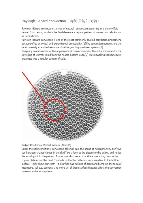
Rayleigh-Benard-convection（瑞利-贝纳尔-对流）Rayleigh–Bénard convectionis a type of natural convection,occurring in a plane offluid heated from below, in which the fluid develops a regular pattern of convection cells known as Bénard cells.Rayleigh–Bénard convection is one of the most commonly studied convection phenomena because of its analytical and experimental accessibility.[1]The convection patterns are the most carefully examined example of self-organizing nonlinear systems[1].Buoyancy is responsible for the appearance of convection cells. The initial movement is the upwelling of warmer liquid from the heated bottom layer.[2] This upwelling spontaneously organizes into a regular pattern of cells.Perfect Conditions, Perfect Pattern (Almost!)Under the right conditions, convection cells will take the shape of hexagons.Why don't we see hexagon-shaped clouds in the sky?Take a look at the picture to the below, and notice the small glitch in the pattern. It was later discovered that there was a tiny dent in the copper plate under the fluid. This tells us thatthe pattern is very sensitive to the bottom surface. Think about our earth - it's surface has millions of dents and bumps in the form of mountains, valleys, canyons, and more. All of these surface features affect the convection patterns in the atmosphere.Fluid in MotionThis picture shows a time lapse view of Rayleigh-Benard cells. The picture was taken over ten seconds, so the aluminum flakes in the fluid look like long trails instead of small particles. This helps to visulaize how the fluid is moving: up through the center of the cell, then spreading out and sinking at the edges of the cell.Development of convectionThe experimental set-up uses a layer of liquid, e.g. water, between two parallel planes. The height of the layer is small compared to the horizontal dimension.At first, the temperature of the bottom plane is the same as the top plane.The liquid will then tend towards an equilibrium, where its temperature is the same as its surroundings. (Once there, the liquid is perfectly uniform: to an observer it would appear the same from any position. This equilibrium is also asymptotically stable: after a local, temporary perturbation of the outside temperature, it will go back to its uniform state, in line with the second law of thermodynamics).Then, the temperature of the bottom plane is increased slightly yielding a flow of thermal energy conducted through the liquid. The system will begin to have a structure of thermal conductivity: the temperature, and the density and pressure with it, will vary linearly between the bottom and top plane. A uniform linear gradient of temperature will be established. (This system may be modelled by statistical mechanics).Once conduction is established, the microscopic random movement spontaneously becomes ordered on a macroscopic level, forming Bénard convection cells, with a characteristic correlation length.Convection featuresConvection cells in a gravity fieldSimulation of Rayleigh–Bénard convection in 3D.（Simulation of 3D Rayleigh-Bèrnard convection with Rayleigh number 10^4 and Prandtl number 1. Temperature is mapped onto the colors of the spectrum, and streamlines are shown in white.）The rotation of the cells is stable and will alternate from clock-wise to counter-clockwise horizontally; this is an example of spontaneous symmetry breaking.Bénard cells are metastable. This means that a small perturbation will not be able to change the rotation of the cells, but a larger one could affect the rotation; they exhibit a form of hysteresis. Moreover, the deterministic law at the microscopic level produces a non-deterministic arrangement of the cells: if the experiment is repeated, a particular position in the experiment will be in a clockwise cell in some cases, and a counter-clockwise cell in others.Microscopic perturbations of the initial conditions are enough to produce a(non-deterministic) macroscopic effect. This inability to predict long-range conditions and sensitivity to initial-conditions are characteristics of chaotic or complex systems (i.e., the butterfly effect).If the temperature of the bottom plane was to be further increased, the structure would become more complex in space and time; the turbulent flow would become chaotic.Convective Bénard cells tend to approximate regular right hexagonal prisms, particularly in the absence of turbulence[3][4][5], although certain experimental conditions can result in the formation of regular right square prisms[6] or spirals[7].The Rayleigh–Bénard InstabilitySince there is a density gradient between the top and the bottom plate, gravity acts trying to pull the cooler, denser liquid from the top to the bottom. This gravitational force is opposed by the viscous damping force in the fluid. The balance of these two forces is expressed by a non-dimensional parameter called the Rayleigh number.The Rayleigh Number is defined as:whereTu is the Temperature of the top plateTb is the Temperature of the bottom plateL is the height of the container.g is the acceleration due to gravity.ν is the kinematic viscosity.α is the Thermal diffusivityβ is the Thermal expansion coefficientAs the Rayleigh number increases, the gravitational forces become more dominant.At a critical Rayleigh number of 1708, the instability sets in, and convection cells appear.The critical Rayleigh number can be obtained analytically for a number of different boundary conditions by doing a perturbation analysis on the linearized equations in the stable state.[8] The simplest case is that of two free boundaries, which Lord Rayleigh solved in 1916.[9] and obtained Rc = 27⁄4 π4 ≈ 657.51.[10] In the case of a rigid boundary at the bottom, and a free boundary at the top (which is the situation in an kettle without a lid), the critical Rayleigh number comes out as Rc = 1,100.65Effects of surface tensionIn case of a free liquid surface in contact with air,buoyancy and surface tension effects will also play a role in how the convection patterns develop.Liquids flow from places of lower surface tension to places of higher surface tension. This is called the Marangoni effect.When applying heat from below, the temperature at the top layer will show temperature fluctuations. With increasing temperature, surface tension decreases.Thus a lateral flow of liquid at the surface will take place, from warmer areas to cooler areas. In order to preserve a horizontal (or nearly horizontal) liquid surface, cooler surface liquid will descend. This down-welling of cooler liquid contributes to the driving force of the convection cells. The specific case of temperature gradient-driven surface tension variations is known as thermo-capillary convection, or Bénard–Marangoni convection.贝纳尔—瑞利对流模型（Benard Rayleigh convective model）是由贝纳尔和瑞利分别通过实验研究提出的有关热对流作用形成机理及其影响因素的、从定性到定量的实验。

搁婴摘要袖：。

丝性约水骧变ｆ』＝ｉ爆过删ｑ，存在各种流体不稳定蛙，它们能够破坏靶丸的别称。

阽羽Ｉ完整性，使得点火火败。

在这些流体力学不稳定性中，瑞利一泰勒不稳定性较容易发，１：，它的破坏性也比较大，被认为是影响惯性约束聚变砸点火所需的最小能：最的０：要凶豢之一，因此深入地理解内爆过程中的瑞利一泰勒不稳定性的发展舭｛ｐ，列于实现点火与商增益聚变是至关重要的。

本文从一个简译的堕逍体模型出发，分别研究了平衡流以及剪切流对瑞４：Ｕ一泰勒不稳定的影ｌ胸，得到如下的结果：１）与波矢平行方向的平衡流会改挛琐烈一泰塑至稳壅的丛塾堡塑堡奎（频移作用）；２）剪叨流及磁场在锐边界条件下对瑞利一泰勒不稳定性的影响表现为：ｉ）瑞利一泰勒不稳定性可以被与扰动波矢平行的５Ｆ衡磁场抑制，如果磁场足够强，瑞利一泰恸不稳定性甚至尢法发展；ｉｉ）与现有的一些模型不同，我们发现剪切流会驱动不稳定性；ｉｉ）Ｉ曲于平衡流剪切的存在，在短波扰动、强剪切流或是较小的阿托伍德＜Ａｆ：，ｗｏｏｄ）数的时候，瑞利一泰勒不稳定性表现出的特性与＂尔文一亥姆稚旌不稳定性类似。

同时，我们给｛“了瑞利一泰勒一；稳定性增长率与扰动波数、约化流剪切、约化Ａｌｆｖｅｎ速度以及阿托伍德数之间的关系。

Ⅵ钮．２，Ｏ岛ｚ、ｆ弓ｊＡＢＳＴＲＡＣＴＡｂｓｔｒａｃｔＴｈｍｔ‘｝ｌｊ’ｔ、ＳＯ１１１３ｕｙｉｎｓ（，献）ｉｌ“ｉ＊ｉｎ１）ｌａ．。

，ｕｌａｔｈａｔｉｎｑ）ｏｓｅｉｎｌｌｃｈＣＯＩＬＳ｛－ｒａｊｉｌｔｏｔｈｅ（）Ｉ，一ＣＩ＇０ｔ．ｉｏｎｏｆｆｕｓｉｏｎＣＯｌｉｌｉｌｌｅｌｌｌｅｕｔｆａｃｉＩｉｔｉｅｓ．ＴｈｕｓｉｔｉｓｉｍｌｘａＩ；ａｎｔｔｏｉｕｖｅｓｔｉｇａｔｅ｛ｈｅｍｌｓｔａｂｌｃｐｒｏｐｍｔｉｅｓ．１ｌｔｎｃｈｏｆｗｈｋ。

１ｌｃａｎｂｅｏｂｔａｉｎｅｄｂｙｅｍＩ）ｌｏｙｉｎｇｔｈｅＭＨＤｍｏｄｅｌＴｈｅｒｅｓｌｆｉｔｓＩｎ‘ｏｖｉｄｅｓＨｉｌｌｎｙ１）ａｓｉｃｉｎｓｉｇｈｔｏｌ’｛．ｈｅｐｈｅ）ｌＯｔｌｌｅｌｌＯｌｌｏｂｓｅｒｖｅ（１ｉｎｌａｂｏｒａ，ｔｏｒｙｃｘｐｅｒｉｎｌｅｔ／ｉｓａｎｄｅｃｌｃｓｔｉａｌｏｂｓｅｒｖａｔｉｏｎｓ．Ｉｎｔｈｉｓｔｈｅｓｉｓ．ｔｈｅｈｅｌｉｃａｌｉｎｓｔａｂｉｌｉｔｙａｎｄＲａｙｌｅｉｇｈ—Ｔａｙｌｏｒｉｎｓｔａｂｉｌｉｔｙｉｓｓｔｕｄｉｅｄａｎｄ８０ｎｌｅｉｎｌｌｏｖａｔｉｏｎａｌ．ｉｍｐｏｒｔａｎｔｒｅｓｕｌｔｓａｒｅｏｂｔａｉｎｅ（】ＴｌｌｅｅｆｒｅｃｔｏｆＩｌｌａｇｎｅｔｉｃｆｉｅｌｄ．ｅｑｕｉｌｉｂｒｉｕｍｆｌｏｗ．ｃｏｍｐｒｅｓｓｉｂｉｌｉｔｙ０１１ｔｈｅｇｒｏｗｔｌｌｒａｔｅｏｆＲａｙｌｅｉｇｈ—Ｔａｙｌｏｒｉｎｓｔａｂｉｌｉｔｙａｒｅｉｎｖｅｓｔｉｇａｔｅｄｉｎｔｈｅｔｈｅｓｉｓ．Ｉｔｃａｎｂｅｃｏｎｃｌｕｄｅｄｔｈａｔ：１１ＯｎｌｙｔｈｅｅｑｕｉｌｉｂｌｉｕｍｆｌｏｗａｌｏｎｇｔｈｅｗａｖｅｖｅｃｔｏｒｈａｖｅｅｆｆｅｃｔｏｎｔｈｅＲａｙｌｅｉｇｈ—Ｔａｙｌｏｒｉｎｓ（，ａｂｉｌｉｔｙａｌｌｄｔｈｅｃｏｎｓｔａｎｔｅｑｕｌｉｌ）ｒｉｎｍｆｌｏｗｗｉｌｌｐｒｏｖｉｄｅａｆｒｅｑｕｅｎｃｙｓｔｒｉｆｔ２１Ｃ０１１３一ｐｒｅｓｓｉｂｉｌｉｔｙｗｉｌｌｓｕｐｐｒｅｓｓｔｈｅＲａｙｌｅｉｇｈ—Ｔａｙｌｏｒｉｎｓｔａｂｉｌｉｔｙ．ＴｈｅｅｆｒｅｃｔｓｏｆｓｈｅａｒｅｄｅｑｕｉｌｉｂｒｉｕｍｆｌｏｗａｎｄｍａｇｎｅｔｉｃｆｉｅｌｄｏｎｔｈｅＲａｙｌｅｉｇｈ－Ｔａｙｌｏｒｉｎｓｔ，ａｂｉｌｉ（，Ｙ（ＲＴＩ）ａｒｅｉｎｖｅｓｔｉｇａｔｅｄａｎｄｔｈｅｌｉｎｅａｒｇｒｏｗｔｈｒａｔｅｉｓｏｂｔａｉｎｅ（１ａｎａｌｙｔｉｃａｌｌｙｉｎｔｈｅｐｒｅｓｅｎｃｅｏｆａｓｈａｒｐｉｎｔｅｒｆａｃ（！．ＩｔｉＳｓｈｏｗｎｔｈａｔｔｈｅｓｈｅａｒｆｌｏｗａｃｔｓａ８ａｄｒｉｖｉｎ￡ｆｏｒｏｅａｌｌ（１ｉｓｔｈｅｄｏｍｉｎａｔｉｎｇｄｒｉｖｅｗｈｅｎＡｔｗｏｏｄｎｕｍｂｅｒＡＴ，ｗａｖｅｕｎｕｌｂｅｒ％，ｆｔｏｗｓｈｅａｒ６ｕａｎｄｇｒａｖｉｔａｔｉｏｎＭａｃｃｅｌｅｒａｌ，ｉｏｎｇｓａｒｉｓｆｙ七（１一Ａ｝）配／以Ｔ》ｇＡｓ，ＬｓｔａｂｉｌｉｚｉｎｇｆａｃｔｏｒｔｈｅｍａｇｎｅｔｉｃｆｉｅｌｄｓｕｐｐｒｅｓｓｅｓＲＴＩａｎｄｗｈｅｎｓｔｒｏｎｇｅｎｏｕｇｈｉｔｅｖｅｎｑｕｅｎｃｈｅｓｔｈｅｉｎｓｔａｂｉｌｉｔｙｔｏｔａｌｌｙ．ＡｓＡＴｉｎｃｒｅａｓｏｓｇｒｏｗｔｈｒａｔｅｉｎｃｒｅａｓｅｓｆｉｒｓｔａｎｄｔｌｌｅｉｌｆａｌｌｓｄｏｗｎｉｆ（２ｋ鹾）＜９ｉｓｓａｔｉｓｆｉｅｄ，ａｌｌｄｏｔｈｅｒｗｉｓｅｉｔｒｉｓｅｓｍｏｎｏｔｏｎｉｅＭｌｙ．Ｗｈｅｎｍａｇｎｅｔｉ（．ｓｔａ¨１ｉｚｉｌｌｚｅｆｆｅｃｔｇｏｖｅｒｎｓ，Ｉ订Ｉｏｎｌｙｏｃｃｕｒｓｉｎｔｈｅｌｏｎｇｗａｖｅｒｅｇｉｏｎａｎｄｎｏｔｏｎｌｙｔｈｅｐｅｎｎｉｔｔｅ（ｉｂａｎｄ，０＜ｋ＜ｇＡ＇Ｉ／［境一鹾（１一Ａ；。

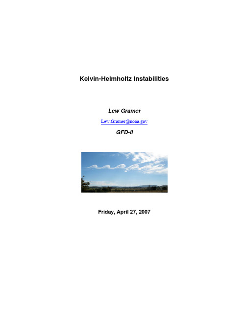
Kelvin-Helmholtz InstabilitiesLew GramerLew.Gramer@GFD-IIFriday, April 27, 2007Table of Contents1. Introduction: The nature of the problem (3)Focus of this paper (3)Further reading (4)2. Scale of Kelvin-Helmholtz instability (4)Vertical scales must be large enough (4)And lateral scales must be small enough (5)But lateral scales must not be too small (5)3. Sufficiency of two dimensions: Squire’s theorem (6)4. Simple conditions for, and limits on shear instability (6)The role of buoyancy: Helmholtz two-layer system (6)An extreme case: The “vortex sheet” (8)The Bernoulli equation: condition for parallel flow stability (9)Evolution into the continuous case (13)5. Continuous profiles: the Taylor-Goldstein equation (14)Necessary condition: Richardson number criterion (16)Why ¼? (Secondary instabilities, turbulence, and mixing) (17)Finding sufficient conditions: empirical studies (18)Limits to growth: Howard’s semi-circle theorem (21)6. Meditations on the Taylor-Goldstein equation (22)The role of viscosity: the Reynolds number (22)Comparison of barotropic and Kelvin-Helmholtz instability (23)Dynamic similarity: lateral and vertical instability (23)7. Importance of Kelvin-Helmholtz instability (25)Surface gravity waves (25)Role in transferring momentum from wind to current (25)Homogenization – ABL and oceanic ML (26)Monin-Obukhov depth scale (26)The “k parameterization” problem (27)Conclusion (28)Acknowledgements (31)References (31)1. Introduction: The nature of the problemThe topic of this paper is the Kelvin-Helmholtz instability, an instability that arises in parallel shear flows, where small-scale perturbations draw kinetic energy from the mean flow. This is inherently a small-scale, irrotational phenomenon, as we will discuss at length below. All of the dynamics that we have studied to date in GFD have been at scales where the Rossby number is small to very small, and thus where rotation is inherently important. However, the dynamics of such larger scale motions in the real world may still depend in critical ways upon smaller scales, where rotation is less important.For this reason, it is important in the context of geophysical systems at least to understand the basic dynamics of small-scale flow as well. This is particularly likely to be true of small-scale motions where there is instability – for intuition tells us that these are precisely the motions that are most likely to modify meso- and planetary-scale dynamics in important ways. And in fact, intuition may even lead us to suspect that small-scale instabilities may play a role in the forcing of larger systems in the real world. As we shall see, both of these intuitions are in fact correct.It is also worth mentioning that the consideration of small scales is an attractive topic in itself. For one thing, it obviates the need to cast our equations of motion in a rotating coordinate frame, greatly simplifying their manipulation. And it leads to another advantage also. We are generally taught by GFD to mistrust conclusions of laboratory experiment and normal physical intuition, as being fundamentally unable to reproduce some of the most important phenomena of large-scale motion. Yet small-scale dynamics not only allows us to use direct experiment. It actually requires us to do so, if we are to derive some of the most important results. And as a corollary, small scales permit us to find very intuitive examples, as we will see.Focus of this paperThe term Kelvin-Helmholtz was originally applied to a particular set of gravity-wave phenomena at discontinuities, originally investigated by von Helmholtz in 1868. Over time, this term has come to refer to a broader class of unstable small-scale motion – including some phenomena that we know do occur in the real ocean and atmosphere. We follow this more general usage in this paper. We must also at the outset distinguish Kelvin-Helmholtz instability from true (small-scale) turbulence. These two phenomena are not truly separable, and in fact, the two play a complex and interactive role in the earth system’s dynamics. However, KHI is a phenomenon that can be adequately considered in two dimensions, as we will see, while turbulence is an inherently three-dimensional phenomenon, and therefore demands a more extensive, sophisticated analysis. Further, our treatment will always assume a basic state of static stability, i.e., that heavier fluid in general lies below lighter fluid. This assumption may not precisely hold in all real geophysical situations, for example in regions of very rapid atmospheric heating from below, or where a fast ocean current interacts with a less dense water mass along a coastal front. However, it does hold in many situations of oceanographic and meteorological interest. And it allows us to ignore the complexity of a phenomenon known as Rayleigh-Taylor instability, when the complexity of the Kelvin-Helmholtz variety is already quite sufficient! So we will choose to assume static stability in all circumstances here. Along the same lines we will sometimes assume – without stating explicitly – that all fluids across a domain are chemically and mechanically miscible. This may bea poor assumption, particularly in the case of ocean wave production by wind. However whenever this assumption may limit important results, I’ll try to indication this assumption explicitly. Finally, the class of motions we choose to study here must be distinguished from the instabilities resulting from an obstruction (e.g., a rough boundary) in a fluid flow. Karman vortex streets and other such phenomena are certainly significant – not only in the laboratory, but also at lateral and vertical boundaries in real geophysical flows. However, they are dynamically distinct from the Kelvin-Helmholtz instability, which by contrast can theoretically occur across any sheared region within a fluid, and so these phenomena will not be considered here.Further readingThe original literature on general Kelvin-Helmholtz instabilities stretches back some 150 years. The most important results are attributed to seminal papers of the last half-century – e.g., Miles (1961), Howard (1961), Klebanoff et al (1962), and Thorpe (1971). Some of these authors were applied mathematicians, using their own particular notation, and many of their derivations can be extremely difficult to follow now. However the subset of these results that we will try to present here is derived in detail, in sections 11.6 through 11.13, of Pijush K. Kundu’s classic Fluid Mechanics (1990). A less rigorous, more intuitive treatment, but one that helps place these results in the context of general geophysics can be found in Cushman-Roisin (1994), sections 11.1 to 11.3. And further applications for KHI in modern geophysical modeling research is found in the upcoming 2nd edition of that eminent text, Cushman-Roisin and Beckers (2007), chapter 14.2. Scale of Kelvin-Helmholtz instabilityVertical scales must be large enough…All the derivations we perform below ultimate rely on regions of sufficiently large vertical extent. We acknowledge however, the possibility that boundaries may play a critical role in the dynamics of small-scale instabilities. An upper boundary (e.g., the free surface of an ocean, for internal KHI), as well as a lower boundary (a flat bottom – or sloped, as will be the case near the wave breaking zone on a coast) is likely to have sometimes a stabilizing, and perhaps sometimes a destabilizing effect on perturbations at a velocity shear. Thus a full treatment of small-scale instability would necessarily have to consider “shallow waves”, as well as complex three-dimensional instabilities. In effect, we would abandon the simple focus we argued for in the introduction! However we are fortunate. For as we will see in the final section of this document, some of the most important real-world applications of KHI occur in regions where we may assume there is no upper or lower boundary. One topic where consideration of small-scale instability is critical is the development of surface waves at the air-sea interface in the open ocean – where we may certainly consider the extent of both sub-domains (air and sea) to be effectively infinite.And as we’ll briefly mention below, another topic where KHI plays a key role is in finding appropriate parameterizations for viscosity in eddy-resolving models of the ocean and atmosphere circulation. Yet here also, away from the narrowest coastal regions of western boundaries, we may hope to be able to allow vertical scales large enough to examine the development of Kelvin-Helmholtz instability, without considering boundaries. As such, we will choose to leave a full treatment of unstable flows within vertically bounded regions – for example, examining the role of inflection points within a mean flow along a theoretical pipe – to the textbooks on fluid mechanics.And lateral scales must be small enough…Horizontally coherent, nearly vertical motions like that pictured on our title page and elsewhere, are observed to occur at very small scales in the real atmosphere and ocean. What is more, experiments over many decades have shown that wave-like instabilities in mean flows can easily be produced that are dynamically identical to these real-world phenomena, but under laboratory setups that have been carefully scaled and controlled to eliminate rotation. We surmise from these two facts, that such instabilities can be driven by very small-scale dynamics, without any reference at all to planetary sphericity or diurnal rotation.We will exploit this observation, to study how such instabilities develop from a purely irrotational system. This is why we made clear in the introduction, that an essential assumption in the development that follows, will be that our motion will consistently remain irrotational – both before and after modification by a perturbation. Therefore, in a real atmosphere or ocean on a rotating planet, this clearly restricts us to characteristic horizontal scales that are much smaller than the effective Rossby radius appropriate to the region of consideration: L << R d*.But lateral scales must not be too small…We have said we will only consider very small scales. And yet throughout this paper, we will choose to ignore the direct effects of such small-scale phenomena as molecular viscosity, surface tension or density diffusion. How can this be reconciled? First, diffusion by molecular processes common in either air or ocean is a slow process over macroscopic scales. Thus for the time scales of real Kelvin-Helmholtz instabilities, we will assume a priori that we may ignore its effect. Second, with respect to surface tension: we will see in a later section that the equation we find to relate a perturbation’s surface displacement to its time evolution is a simple first-order one. Yet surface tension introduces an additional term into this equation, which is of second order in displacement. The net effect of this change is to modify the effect of gravity in the dispersion relation between frequency and wavelength: In effect, surface tension acts as an additional restoring force in wave dynamics. Interfacial waves where molecular surface tension plays an equal or dominant role relative to gravity are generally referred to as capillary waves.These waves are the inevitable first “fillip”, likely to precede the development of some larger-scale instabilities. However, it can be shown (Kundu sec. 7.7) that for perturbations of wavelength greater than a certain small value (λ ≈7cm for example, at the air-sea interface), Kelvin-Helmholtz instabilities can still progress, while surface tension may be ignored. Thus for fluid interfaces, we must limit our study below to the further development of instabilities after an initial unstable perturbation has developed. By this assumption we may ignore capillary waves from this point forward. Yet it will be worthwhile for the reader to bear in mind this lower limit on wavelength (i.e., upper limit on wavenumber), when we derive criteria for wave instability in section 4 below. Finally, molecular viscosity is likely to play an important role in small-scale instabilities: below we will try to decompose its stabilizing or destabilizing effect in the absence of stratification.3. Sufficiency of two dimensions: Squire’s theoremIn the examples throughout this paper, we ignore the second horizontal dimension. We are in fact about to derive a set of bounds and criteria for instability in small-scale perturbations, relying on two-dimensional governing equations. How can we be sure that any bounds or conditions on instability that we derive from such an analysis will also hold in real, three-dimensional flows? For this, we rely on an important and striking result known as Squire’s theorem (Squire 1933). This theorem actually relies on a coordinate transform in wavenumber space. The result is a simplification of the normal mode analysis, which Squire uses to show that – for each unstable three-dimensional wave solution to a perturbed system, there must always exist a two-dimensional wave solution which is unstable at higher wavenumber. In other words, a two-dimensional system is always more unstable than any equivalent three-dimensional system, using the same analysis! The transformation is a brilliantly simple one, with pure horizontal wavenumber for the 2-D system defined by the transformation κ = (k2 + m2)1/2, while total (complex) phase speed c remains the same. Squire demonstrates that in the Flatlandian system, unstable perturbations of the transformed two-dimensional momentum equations will grow as exp(κc i), whereas three-dimensional disturbances are confined to grow at the rate kc i, where by definition kc i≤κc i. Squire’s theorem tells us that KHI and, as we will see, pure barotropic instability also, can be fully described and analyzed using equations in two dimensions. It is important to note in passing what this means: for not only is this a trick for simplifying stability analysis. Rather, the theorem defines for us a dynamic similarity, such that we may say in effect, that all instabilities in parallel mean flows are inherently two-dimensional. We will analyze the implications of this below.4. Simple conditions for, and limits on shear instabilityThe role of buoyancy: Helmholtz two-layer systemWe will follow Cushman-Roisin, by first doing a simple analysis of the classic two-layer system based on energetics, to derive a natural condition that must me met if instability in this system can possibly lead to mixing. We’ll see that here, as above, instability is always possible for sufficiently short perturbation scales. (This statement however, may be less complete than we wish. To wit, see our earlier discussion on the restoring – i.e., instability-dampening – role of surface tension.) In this section, we consider a two-dimensional domain infinite in vertical and horizontal extent. This two-layer system is essentially that which was considered by Hermann von Helmholtz.We first posit a priori that conditions do exist which allow instabilities to derive energy from the shear (U2-U1) in our mean flow. We further consider that these instabilities ultimately lead to mixing of the fluid over some finite vertical distance ∆H in the domain, centered on the initial discontinuity. This in turn results in a net gain in potential energy within the mixed region. The resulting mixed region is shown in the figure below, adapted from Cushman-Roisin 2007.Time Æ We then ask what conditions must be met by the resulting energy balance, in order for us tovalidate these assumptions. (Note this differs trivially from the treatment in Cushman-Roisin, only in that we do not assume vertical boundaries to our system. These in fact prove to play no role in the dynamics of the developing instability, under our energetic analysis.)We may characterize the available potential energy in our initial or basic system by the integrals:434404212122212121212122212/12/02H g H g H g H g H g dz gz dz gz HH H ∆−∆=∆⋅−∆+−∆=⋅+⋅∫∫∆∆∆ρρρρρρρFrom this, based on our assumption of mixing over the length ∆H , we develop into a final state with the following net gain in potential energy 21281)(H g PE ∆⋅−=∆ρρ. We understand that thenet gain in PE can only be accomplished in this (or any similar) system by a corresponding loss in kinetic energy from the sheared mean flow. By a similar vertical integration across ∆H for our initial and final states, this minimal conversion of kinetic energy to potential energy is found to beH U U KE ∆−=∆2121)(ρ. Here we define 2/)(12ρρρ+=, 2/)(12U U U +=, and we have further assumed per Boussinesq that 21ρρρ≈≈ for simplicity.For mixing to occur – as we propose that it inevitably must from an unimpeded unstable perturbation – our simple energetic analysis leads thus to the following necessary condition: 21212)()(U U H g −≤∆⋅−ρρρ (4.0) It is important to be clear that this inequality represents an upper bound on the transfer of mean flow kinetic energy required to achieve fluid mixing. As we will see later in the section on the Richardson number criterion, the inequality above clearly does not represent a least upper bound on that energy requirement. The weakness of this result can partly be attributed to the unrealistic nature of the inviscid, narrow scale-range discontinuities we are considering here; this point is nicely illustrated by the pathological example in the next sub-section.However, this weakness is really due to the fact that mixing , under the assumptions we’ve made, is not adequately explained by two-dimensional phenomena like KHI – even if they are allowed to become fully non-linear. We will hopefully discuss this further, albeit briefly in the final section.An extreme case: The “vortex sheet”A curious conclusion can be drawn from inequality (4.0). Imagine a simple system where a plane discontinuity separates two regions of parallel flow, both of the same density. In this scenario, if mixing occurs then the loss of potential energy will actually be zero. This implies that the inequality above will always be satisfied. Any perturbation in the planar discontinuity however slight should draw sufficient kinetic energy from the shear discontinuity to develop indefinitely. This is especially so for non-horizontal plane discontinuities – where we may expect any potential energy barrier to shear instability to be even smaller with increased angle from the vertical.Note that this places no constraints on the transfer of kinetic energy from the sheared mean flow either. In fact, we might presume that in the absence of momentum diffusion, the instability and resulting mixing would in fact cause no net change in total kinetic energy of the system at all! Naturally though, as the instability develops, transitions to secondary instabilities, and ultimately to turbulence and mixing, the scales of the motion (and of the energy of the system) would change. To continue our discussion, we have just concluded that where a fluid has no variation in density within a region, then instability will theoretically always be present where ever there is a shear discontinuity. This simple setup is known as a “vortex sheet” for obvious reasons, and represents an extreme case in the analysis of Kelvin-Helmholtz instability. Yet consider that homogenous water columns, over small scales at least, are actually quite common in the ocean: indeed they are a natural result of the very dynamics we study in this paper!Why then do we not observe “vortex sheets” wherever there is shear in the mean flow over a homogeneous region? To answer this question, we need only recall our decision at the outset, to ignore surface tension and boundaries, and to decouple viscosity from the effects of buoyancy. All of these factors can set constraints on the development of small-scale instability, even where buoyancy is minimal. And as this argument implies, I believe these effects must play quite a significant role in the real world, particularly in the air-sea interface and oceanic mixed layer.The Bernoulli equation: condition for parallel flow stabilityWe continue with the two-layer system, and seek to derive appropriate condition for instability by considering a wave-like perturbation at a discontinuous interface between two fluids, as a solution to Euler’s irrotational momentum equations. This setup is summarized by the figure below:Figure 1: Kelvin-Helmholtz instability developing from a wave-like perturbation of wavenumber k at the interface between two vertical regions (a); resulting in breaking (b), and ultimately in mixing like that which we assumed a priori in the previous section. (Figure from Cushman-Roisin and Becker 2007.)We develop this example at length, as it is intuitive and easy to manage. Further it will prove to be an illustrative preliminary when we consider the more realistic case of a continuous distribution of both velocity and density in the sections below on the Taylor-Goldstein equation and theRichardson number criterion. For we will find that that famous criterion begins from essentially the same equations, subject only to somewhat different boundary conditions across the interface. We have assumed that our horizontal domain scale is small relative to the Rossby radius; a motion uniform over a domain, whose shear is zero, may be considered to have zero absolute vorticity as well. This condition allows us to characterize the momentum balance in our two-dimensional system using the relatively simple Euler equations : x p z u w x u u t u ∂∂−=∂∂+∂∂+∂∂ρ1, g z p z w w x w u t w −∂∂−=∂∂+∂∂+∂∂ρ1. (4.1)For barotropic motions (ρ ≡ ρ(p)) like that of our basic state, these momentum equations lead to the following system of equations for the lateral and vertical energy balance of our system: x u dp q x t u )(221ζρ×=⎥⎦⎤⎢⎣⎡+∂∂+∂∂∫r , z u gz dp q z t w )(221ζρ×=⎥⎦⎤⎢⎣⎡++∂∂+∂∂∫r . (4.2) For scales much less than the appropriate Rossby radius the basic state is irrotational , which means that the right side of both these equations will be zero. This fact allows us to conclude that Bernoulli’s equation (see below), which generally states the conservation of total energy along streamlines, will in fact hold uniformly everywhere within the system under consideration. We characterize the basic balance of pressure P i , with kinetic and potential energy within each sub-domain by using by these conservation relations at all levels (∀z) in the domain:1112121C gz P U =++ρ, 2222221C gz P U =++ρ, with C 1,C 2 constant.From which we derive a simple boundary condition at the interface between the domains, z = 0:)()(222212121211C U C U −=−ρρ.(4.3)We now introduce at time t =0 a perturbation to the interface between these domains. If it issufficiently small, but again in absence of viscosity, diffusion and other non-linear effects we have chosen to ignore, Kelvin’s Circulation theorem tells us that the resulting system will still be irrotational . In words, we require a fluid where net viscous forces vanish uniformly throughout the domain (we have actually required an inviscid fluid ), and where there is no stratification away from the interface. In such a system, we state that any wave-like perturbation with a frequency much greater than the local Coriolis frequency (and length scale sufficient to ignore dissipation, diffusion, and surface tension) will have no relative vorticity .To place these considerations in mathematical terms, we have defined a basic state and subjected it to a certain class of perturbations, such that the resulting system can be characterized by two-dimensional velocity potential functions φ~1,2 within each region: 111~φφ+=x U , 222~φφ+=x U . (4.4) And further these functions will by definition obey the homogeneous Laplace equation : 0~12=∇φ, 0~22=∇φ.We have in the process defined our perturbations in such a way that they are therefore also characterized by potential functions, satisfying their own perturbation Laplace equations: 0,. 12=∇φ022=∇φ(Note that a velocity potential function defines a scalar field, the components of whose gradient defines two components of velocity. Where the flow is irrotational, as is the case here, the velocity potential function completely defines fluid motions in the system, as: u ≡∂φ/∂x, and v ≡∂φ/∂y.) We now subject the system to boundary conditions – the first of which is the rather weak condition that this small-scale perturbation must be finite in vertical extent:01→φ as , ∞→z 02→φ as −∞→z .We next require a somewhat more stringent “kinematic” boundary condition, namely, continuity at the interface. We in effect require that fluid, which is initially at either side of the interface between the upper and lower layers, will remain at that interface as it develops: yv x u U t dt d z ∂∂+∂∂++∂∂==∂∂ζζζζφ1111)( at z = ζ-, and y v x u U t dt d z ∂∂+∂∂++∂∂==∂∂ζζζζφ2222)( at z = ζ+.We here restrict the scale of our perturbation still further, by requiring that it be small enough for non-linear terms in the perturbation velocities to be ignored – when we examine fluid parcel motion at the basic interface at z=0. We thereby simplify the above conditions to:x U t z ∂∂+∂∂=∂∂ζζφ11 at z = 0, x U t z ∂∂+∂∂=∂∂ζζφ22 at z = 0. (4.5)We stated above a general constraint (4.3) on pressures in the basic flow state. Let us now look a little closer at how pressure will be distributed across the perturbed interface. For note that in this theoretical example, we have considered a fluid with discontinuous density and velocity interfaces. But if our system is to be mathematically tractable and further is to have any relationship at all to realistic situations, we must assume that pressure distribution across the system is continuous. We are thus lead to state as a further boundary condition that the pressures on both sides of our perturbed interface will smoothly approach the same limit.To arrive at this condition, we first consider the balance between pressure and energy terms in the perturbed system, above and below the interface. Thanks to our many careful assumptions, we may state these balances in terms of the unsteady Bernoulli equation (Kundu 4.15):11121211~)~(~C gz p t =++∇+∂∂ρφφ, 22222212~)~(~C gz p t =++∇+∂∂ρφφ. (4.6) From the above equation, it is obvious where our statement of the basic (pre-perturbation) pressure balance (4.3) came from. However, we now strengthen that balance, requiring that the perturbationpressures across the interface also be continuous: 1~p =2~p at z=ζ. We must restate this condition in terms of the potential functions and interface displacement. We can do this by restating the unsteady Bernoulli equations in terms of our decomposition (4.4), and combining the two equations into a single linear condition at z =ζ:[][]⎥⎦⎤⎢⎣⎡−+++−∂∂−=⎥⎦⎤⎢⎣⎡−+++−∂∂−ζφρζφρg w v u U t C g w v u U t C 222222221222212121121111)()( (4.7) Again utilizing the scaling of our perturbation to restate this as a linear condition at the basic interface, z=0, we then subtract our original basic state boundary condition 4.3 to simplify:⎥⎦⎤⎢⎣⎡+∂∂+∂∂=⎥⎦⎤⎢⎣⎡+∂∂+∂∂ζφφρζφφρg x U t g x U t 22221111, at z = 0. (4.8)Now we follow a procedure that will by now be very familiar to any student of large- and meso-scale geophysical dynamics. We assume that a vertically and horizontally decoupled linear solution to this system may exist, allowing us to solve for all three of our variables above:()()kz kz i r ct x ik Be Ae and ic c c but k where e −−−==+=ℜ∈=21)(2121,,,,,,,,φφφφζφφζ))))) (4.9) (In the expressions for the lower and upper vertical perturbation modes, recall we linearized our interface conditions to the level of the initial interface at z=0!) Our “kinematic” boundarycondition (4.5) of continuity at the interface then gives us immediately these solutions for A and B: ζ))(1c U i A −−= ζ))(2c U i B −= (4.9a) Substituting this with our presumed complete solutions into the unsteady Bernoulli equation, we derive an expression relating our phase speed c to the horizontal wave number k :()()()12211222ρρρρ−=−+−g c U k c U k , (4.10)Which we can easily solve for a direct expression of the (complex) phase speed, as:2/121212************⎥⎥⎦⎤⎢⎢⎣⎡⎟⎟⎠⎞⎜⎜⎝⎛+−−+−±+−=ρρρρρρρρρρρρU U k g U U c . (4.11)Clearly we find that c will have a non-zero imaginary part only in the case where the first term within the square-root is less than the second term. For a stably stratified system (ρ2>ρ1), this can only occur when U 2 ≠ U 1. From this it follows that our necessary criterion for mixing must be: g (ρ22 - ρ12) < k ρ1ρ2 (U 2 - U 1)2. (4.12)。

PY542INFORMATION Fall2008Instructor:Sidney Redner(321SCI,x2618)Office Hours:Tues.&Fri.9-10:30am,and by appointment.General:This course treats non-equilibrium statistical mechanics and transport phenom-ena.Because of the rapid developments in thefield,the breadth of topics,and the lack of an established formalism,most of the classic texts no longer seem appropriate for this course.For this reason,the“unofficial”course text is a book that I am currently writing with2co-authors.It is continuously being updated and individual chapters are posted on the course website.Other books that should be helpful during the semester include:(i)N.G.Van Kampen,Stochastic Processes in Physics and Chemistry(North-Holland). This gives an excellent treatment of stochastic processes.Buy it used if you can.I would have assigned this as the text if the price was a factor2smaller.(ii)S.Redner,A Guide to First-Passage Processes(Cambridge University Press).This book gives background on random walks and diffusion processes,as well as a reference for the portion of the course onfirst-passage phenomena.If you purchase the hardcover version,I will refund you my royalty(approximately$5.50per book),but the paperback version is much cheaper.I will also post relevant excerpts on the course website. (iii)F.Reif,Statistical and Thermal Physics(McGraw-Hill).A standard advanced un-dergraduate text for statistical mechanics.The last few chapters provide a particularly useful introduction to various aspects of non-equilibrium processes.(iv)K.Huang,Statistical Mechanics2nd edition(Wiley).Relevant chapters are3and 5that deal with kinetic theory and transport phenomena.(i)N.Wax(editor),Selected Papers on Noise and Stochastic Processes(Dover).This book contains reprints of some of the most important classic research articles on stochas-tic processes.Although out of print,it may be possible to obtain used somewhere.How-ever,the book contains reprints of articles that are generally available on the web.The most useful is“Stochastic Problems in Physics in Astronomy”by S.Chandrasekhar, Rev.Mod.Phys.15,1–89(1943).Other useful articles include“On the Theory of the Brownian Motion”,by G.E.Uhlenbeck and L.S.Orenstein,Phys.Rev.26,823–41(1930)&“On the Theory of the Brownian Motion II”by M.C.Wang and G.E. Uhlenbeck,Rev.Mod.Phys.17,323–42(1945).(v)R.Kubo,M.Toda and N.Hashitsume,Statistical Physics II(Springer-Verlag). Contains a particularly good discussion of linear response theory and thefluctuation-dissipation theorem.(vi)J.A.McLennan,Introduction to Non-Equilibrium Statistical Mechanicsi(Prentice-Hall).This book contains a thorough discussion of the Boltzmann transport equation. (vii)H.J.Kreuzer,Non-Equilibrium Thermodynamics and its Statistical Foundations (Oxford University Press).Comprehensively treats transport theory from the macro-scopic viewpoint and has an excellent discussion of the Rayleigh-B´e nard instability.Course organization:Lectures:Lectures will be held on Tuesdays and Thursdays from2:00—3:30in SCI B58.The accompanying outline represents a rough approximation to the material that will be covered this semester.Discussion:Sections will be held weekly starting Wed.Sept.3at2:00pm in PRB365.Homework:Approximately10assignments will be handed out.While some collab-oration on homework is acceptable,what is turned in should represent your personal effort.Exams and Grading:The average of the homeworks will count approximately30±5% of the total class grade.I will give one midterm exam(exact format to be determined) that will count approximately30±5%of the total class grade.For thefinal,I am currently planning a take-home but time-limitedfinal exam that will count for the approximately remaining40%of the total course grade.。

酷炫动图（三十四）：表面张力，“膜”的力量科学人果壳网科技有意思膜在生活中可是见得太多了，大家对膜都非常熟悉，水滴表面、肥皂泡等都是常见的“膜”。

但是你了解膜背后的理论吗？今天，我们就一起来提高姿势水平，学习一下“膜”的力量——表面张力。

首先，什么是表面张力？要解释表面张力，我们首先要走进微观世界，看看那些液体分子之间是如何互动的：现在我们选一个处于液体内部的水分子，对，就你，最萌的那个：因为无论往哪个方向看，看到的都是相同密度的水分子，所以吸引力和压强对于它来说都是平衡的。

现在，让我们把上半部分的水换成空气：假设上下两部分的压强相同（压强不同的情况将在第二节介绍），由于空气对水分子的吸引力小于水分子之间的吸引力，所以位于表面的水分子会受到指向液体内部的力，一部分水分子被拉进液体内部，表面层的水分子开始变稀疏，直到吸引力减弱到和空气接近时趋于平衡。

表面层水分子的间距大于r0 ，因此吸引力占上风：表面张力就是液体表面层水分子之间的吸引力（不是垂直于表面把水分子往里拉的那个力）。

这个力使液体表面像一个绷紧的橡皮膜，表面张力系数σ 的第一种定义就是：作用在液面单位长度上的张力的大小，单位为N/m。

具有“橡皮膜”一般特性的肥皂水液膜。

戳破一边后，另一边在表面张力的作用下迅速回缩。

录制者：Jubobroff垂直于液面的拉力使表面的水分子具有了势能，称为表面自由能（不引起混淆时可简称为表面能）。

当你克服表面张力扩大液体的表面积时，实际上是做功提升一部分原本位于内部的水分子来到表面（相应的，缩小表面积可对外做功），这样就有了表面张力系数σ 的第二种定义：单位面积的表面能，单位J/m2 。

这两种定义是等价的，以下我们既可以通过分析表面张力得出结论，也可以通过液体“希望”自己表面能最小的角度得出相同的结论。

膜为什么这样弯如果界面两侧有气压差，膜就会弯曲以平衡气压差，气压高的一侧会使膜向气压低的一侧凸出，这就是吹泡泡的原理。

Lecture 8 Rayleigh InstabilityRayleigh (1878) examined a common experience: a thin jet of liquid is unstable and breaks into droplets. When a jet is thin enough, the effect of gravity is negligible compared to surface energy. The jet changes its shape to reduce the total surface energy. Liquid flow sets the time.Similar instability in solids. Phenomena similar to the Rayleigh instability occur in solid state; see Rodel and Glaeser (1990) for an experimental demonstration and for a literature survey. For example, at a high temperature, a penny-shaped pore in a solid first blunts its edge, from which finger-like tunnels emerge, and the tunnels then break into small cavities (Lange and Clarke 1982).Why does a cylinder evolve into a row of droplets? Srolovitz and Safran (1986) gave a simple geometric argument. Assume that the surface energy density is isotropic, and the free energy of the system is the surface area times the surface tension. One has to show is that the cylinder has a larger surface area than the row of spheres. Consider a long cylinder of radius R, and a row of droplets, each of radius b. Imagine that the cylinder evolves to the droplets by first perturb the surface with a wavelength λ. The volume per wavelength of the cylinder equals the volume of each droplet, so that the droplet radius is given by()1/3.b=3R2λ/4The free energy per wavelength of the cylinder is 2πRλγ. The free energy per droplet is .4πb2γThe free energy of cylinder is larger than the row of droplets ifλ>9R/2.From this geometric (energetic) consideration, one expects that a fiber can evolve to a row of spheres of large enough radii.2RBut wait. Doesn't a single big sphere have the smallest surface area? Why does the cylinder evolve to many small droplets, rather than a single large sphere? The energetic consideration does not answer this question. The answer has to do with kinetics. It takes a short time for the cylinder to evolve to a row of spheres. When the cylinder evolves into droplets, mass transport stops, preventing the system from reaching the minimal energy configuration, a single large sphere. Here we have assumed a certain kind of mass transport mechanism, such as fluid flow or solid diffusion. If, instead, the cylinder is sealed in a small bag, it will evolve to a single large sphere via vapor transport.Why do atoms diffuse from the troughs to crests? I always thought that a smooth surface has a low free energy. For the cylinder to evolve to droplets, it must first become wavy.Why do atoms diffuse from the troughs to crests? The answer has to do with a simple geometric fact: the cylinder lives in three dimensions. At each point on the surface there are two principal curvatures: one corresponds to the circle in the section normal to the cylinder axis, and the other corresponds the wave in the section along the cylinder axis. We will call the two curvatures and . At a trough, the circle is small. At a crest, the circle is big. Consequently, the difference in drives atoms to diffuse from the trough to the crest, amplifying the wave amplitude. On the other hand, is positive at a crest, and negative at a trough, so that the difference in drives atoms to diffuse from the crest to the trough, decreasing the wave amplitude. The difference in is small when the wavelength is very long.1K 2K 1K 2K 2K 2K How fast will the cylinder evolve? To answer this question requires us to study the mass transport process. Perturb the radius of the cylinder in the form:()()()[]kz t R t r r cos 1,ε+=We will carry out a linear perturbation analysis. We retain terms linear in the perturbation amplitude ε.The surface has two principal curvatures. One curvature is the inverse of the radius of a cross section:()[]kz Rr K cos 1111ε−==. For the cylinder of the wavy surface, the curvature increases at troughs, and decreases at crests. The other curvature is in the cross-section of the cylinder along the axial direction:()kz Rk zr K cos 2222ε=∂∂−=. This curvature is negative at troughs, and positive at crests. As discussed before, the two principal curvatures have the opposite trends.The surface velocity is ()kz tR t r v n cos ∂∂=∂∂=ε In the governing equation , for the small perturbation, the surface Laplacian is , so that(212K K B v n +∇=)222/z ∂∂=∇ τεε=dt d , with()()424/kR kR B R −=τ . This is an ordinary differential equation for the wave amplitude ()t ε. For the initial condition ε=ε0() at t = 0, the solution to the ordinary differential equation isεt ()=ε0()exp t /τ().This shows how fast the wave amplitude will change.Wavelength selection. The characteristic time τ varies with the wavelength. When λ<2πR , the perturbation increases the free energy, τ < 0, and the perturbation diminishes with the time. When λ>2πR , the perturbation decreases the free energy, τ > 0, and the perturbation amplifies with the time. A very long wavelength, mass transport over a long distance takes a long time. Consequently,τ minimizes at an intermediate wavelength, given by R m πλ22=. If perturbations of all wavelengths have an identical initial amplitude, ε0(), the perturbation of wavelength λm grows most rapidly at t = 0. It is often assumed that this wavelength would win the race even at later times, and the fiber eventually breaks at this wavelength.0C H A R A C T E R I S T I C T I M E τΩ2M s γR 4The time scale . Corresponding to the fastest growing wavelength, the characteristic time is.B R m /44=τThis is the time scale for the Raleigh instability to occur. We could have obtained this scaling from dimensional considerations. Recall that kT D B s s s /δγΩ=. The Rayleigh instability occurs over a long time if the radius is large or the temperature is low.The above conclusion is made on the basis of the linear stability analysis, where high order terms of ε have been ignored. A complete simulation of the surface evolution is necessary to take into account of the actual initial imperfection and large shape change (Nichols 1976). Yu and Suo (1999) developed a finite element method to evolve axisymmetric surfaces.ReferencesLord Rayleigh, Proc. Longon Math. Soc. 10, 4 (1878).Lange, F.F. and Clarke, D.R. (1982) Morphological changes of an intergranular thin film in a polycrystalline spinel. J. Am. Ceram. Soc. 65, 502-506.Nichols, F.A. and Mullins, W.W. (1965) Surface- (interface-) and volume-diffusion contribution to morphological changes driven by capillarity, Trans. Metall. Soc. 233, 1840-1848.Nichols, F.A. (1976) On the spheroidization of rod-shaped particles of finite length, J. Mater.Sci.11, 1077-1082.Rodel, J. and Glaeser, M. (1990) High-temperature healing of lithographically introduced cracks in sapphire. J. Am. Ceram. Soc. 73, 592-601.Srolovitz, D.J. and Safran, S.A. (1986) Capillary instabilities in thin films. J. Appl. Phys.60, 247-260.H.H. Yu and Z. Suo, An axisymmetric model of pore-grain boundary separation. J. Mech. Phys.Solid., 47, 1131-1155 (1999).。