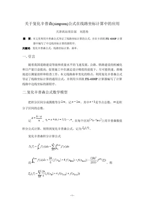
复化辛普森公式英文
- 格式:docx
- 大小:37.07 KB
- 文档页数:3
复化辛普森公式英文
The Simpson's Composite Rule Formula
The Simpson's Composite Rule is a numerical integration method used
to approximate the definite integral of a function. It provides a way to
calculate the area under a curve by dividing it into smaller intervals and
applying a specific formula. In this article, we will discuss the Simpson's
Composite Rule, its derivation, and how it can be applied in practice.
Introduction to the Simpson's Composite Rule
The Simpson's Composite Rule is an extension of the Simpson's Rule,
which is used to approximate definite integrals using quadratic
approximations. The main idea behind the Simpson's Composite Rule is to
divide the interval of integration into multiple subintervals and apply the
Simpson's Rule on each subinterval. By summing up the individual
approximations, we can obtain a more accurate approximation of the definite
integral.
Derivation of the Simpson's Composite Rule
To derive the Simpson's Composite Rule, we start by dividing the
interval of integration into n subintervals. Each subinterval has a width of h,
which is calculated by dividing the total width of the interval by the number
of subintervals (h = (b - a) / n, where a and b are the lower and upper limits
of integration, respectively). Next, we apply the Simpson's Rule on each subinterval, using three
equally spaced points to construct a quadratic approximation. The formula
for the Simpson's Rule can be expressed as:
∫[a,b]f(x)dx ≈ (h/3) * [f(x0) + 4f(x1) + f(x2)]
where x0, x1, and x2 represent the endpoints of each subinterval.
By integrating the function over each subinterval and summing up the
results, we obtain the Simpson's Composite Rule formula:
∫[a,b]f(x)dx ≈ (h/3) * [f(x0) + 4f(x1) + 2f(x2) + 4f(x3) + ... + 2f(x(n-2)) +
4f(x(n-1)) + f(xn)]
where xn represents the endpoint of the last subinterval.
Example Application
Let's say we want to approximate the definite integral of the function f(x)
= x^2 within the interval [0, 2], using the Simpson's Composite Rule with 4
subintervals.
First, we calculate the width of each subinterval:
h = (b - a) / n
= (2 - 0) / 4
= 0.5
Next, we evaluate the function at the endpoints and midpoint of each
subinterval:
x0 = 0, x1 = 0.5, x2 = 1, x3 = 1.5, x4 = 2 f(x0) = 0, f(x1) = 0.25, f(x2) = 1, f(x3) = 2.25, f(x4) = 4
Finally, we substitute these values into the Simpson's Composite Rule
formula:
∫[0,2]x^2 dx ≈ (0.5/3) * [0 + 4*(0.25) + 2*1 + 4*(2.25) + 4]
= (0.5/3) * [0 + 1 + 2 + 9 + 4]
= 0.5 * [16/3]
≈ 2.67
Therefore, the approximate value of the definite integral is 2.67.
Conclusion
The Simpson's Composite Rule is a powerful numerical integration
method for approximating definite integrals. By dividing the interval of
integration into multiple subintervals and applying the Simpson's Rule on
each subinterval, we can obtain a more accurate approximation. This method
is widely used in various fields, including physics, engineering, and finance,
where numerical integration is necessary. It is important to note that the
accuracy of the approximation improves as the number of subintervals
increases.