Nonlocal Effect of Local Nonmagnetic Impurity in High-Tc Superconductors Induced Local Mome
- 格式:pdf
- 大小:100.29 KB
- 文档页数:3


nonlocal结构
Nonlocal结构是指结构中存在着非局部效应的现象。
在传统的局部效应结构中,结构的受力和变形只与其周围的局部构件有关,而非局部效应结构中则存在着信息的非局部传递和作用,也就是说,结构的受力和变形不仅与其周围的局部构件有关,也与结构内部和远离结构的区域有关。
非局部效应的存在使得结构的设计和分析变得更为复杂。
在材料的选择和结构的组装中,需要考虑非局部效应对结构的影响,同时在结构的分析和优化中也需要考虑非局部效应的影响。
因此,非局部效应的研究和理解对于结构设计和分析具有重要的意义。
目前,非局部效应的研究主要涉及到物理学、数学和工程学等领域。
在物理学中,非局部效应主要涉及量子力学和相对论等领域;在数学中,则涉及到非局部微积分和非局部偏微分方程等内容;在工程学中,非局部效应的研究主要集中在结构力学、材料力学和计算力学等领域。
尽管非局部效应的研究还存在着一些挑战和困难,但其在结构设计和分析中的重要性已经得到了广泛的认识和重视。
未来,随着技术的不断进步和理论的不断完善,非局部效应的研究将会取得更加深入和广泛的进展。
- 1 -。

埃农映射的不动点埃农映射(Arnold's cat map)是一种具有周期性的非线性映射,最早由Vladimir I. Arnold在1968年引入,用来说明质点在二维平面上的运动轨迹。
这个映射的非线性特点使得它具有许多有趣的数学性质,其中之一是存在不动点。
埃农映射可以形象地理解为将一个正方形的平面划分为一个个小的正方形,并按照一定的规则对小正方形进行旋转和重新排列,从而得到新的平面。
这个过程可以表示为一个二维的矩阵乘法。
具体而言,给定一个矩阵```A = [[2, 1],[1, 1]]```和一个二维向量```X = [x, y]```则埃农映射可以表示为```A * X (mod 1)```其中mod 1表示取余数。
根据埃农映射的定义,我们可以通过反复将一个点进行映射来观察它在平面上的运动轨迹。
令一个初始点为(X0, Y0),经过n次映射后得到(Xn, Yn)。
当(Xn, Yn) = (X0, Y0)时,我们称它为一个周期为n的不动点,表示在n次映射后,点回到了初始的位置。
埃农映射具有非常有趣的周期性特征。
事实上,对于一个正方形的平面而言,埃农映射的周期为n的不动点共有n个。
这意味着在平面上存在很多很多的周期性轨迹,这些轨迹之间又有着复杂的交织关系。
这种周期性特征是埃农映射非线性性质的直接体现,也是它被广泛研究和应用的原因之一。
埃农映射及其不动点的研究在许多领域中都有重要的应用。
在动力系统中,埃农映射是研究混沌现象的一个重要模型。
混沌现象是指非线性动力系统中出现的无规律、无周期的运动。
埃农映射的周期特性使得它成为理解混沌现象的基础模型之一。
在密码学中,埃农映射的周期性特征被应用于设计密码算法。
利用埃农映射的特性,可以生成一系列随机数,并通过一定的操作将这些随机数转化为密码所需的扰动序列。
这种基于埃农映射的密码算法被广泛应用于信息安全领域。
此外,在图像处理和数据压缩领域,埃农映射也有一定的应用。
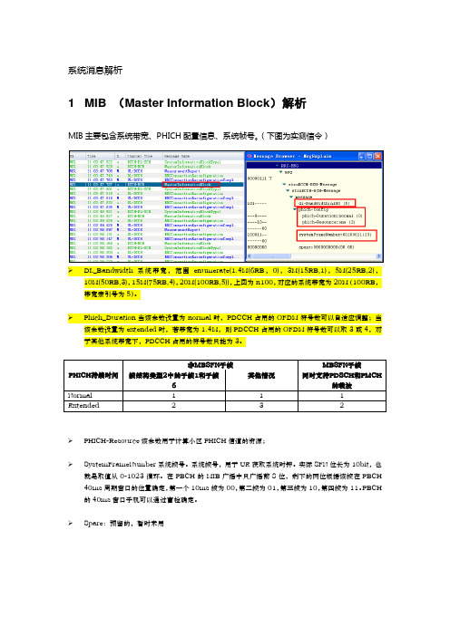
系统消息解析1 MIB (Master Information Block)解析MIB主要包含系统带宽、PHICH配置信息、系统帧号。
(下图为实测信令)➢DL_Bandwidth系统带宽,范围enumerate(1.4M(6RB,0),3M(15RB,1),5M(25RB,2),10M(50RB,3),15M(75RB,4),20M(100RB,5)),上图为n100,对应的系统带宽为20M(100RB,带宽索引号为5)。
➢Phich_Duration当该参数设置为normal时,PDCCH占用的OFDM符号数可以自适应调整;当该参数设置为extended时,若带宽为1.4M,则PDCCH占用的OFDM符号数可以取3或4,对于其他系统带宽下,PDCCH占用的符号数只能为3。
➢PHICH-Resource该参数用于计算小区PHICH信道的资源;➢SystemFrameNumber系统帧号。
系统帧号,用于UE获取系统时钟。
实际SFN位长为10bit,也就是取值从0-1023循环。
在PBCH的MIB广播中只广播前8位,剩下的两位根据该帧在PBCH 40ms周期窗口的位置确定,第一个10ms帧为00,第二帧为01,第三帧为10,第四帧为11。
PBCH 的40ms窗口手机可以通过盲检确定。
➢Spare:预留的,暂时未用2 SIB1 (System Information Block Type1)解析SIB1上主要传输评估UE能否接入小区的相关信息及其他系统消息的调度信息。
主要包括4部分:➢小区接入相关信息(cell Access Related Info)➢小区选择信息(cell Selection Info)➢调度信息(scheduling Info List)➢TDD配置信息(tdd-Config)SIB1消息解析(UE侧):RRC-MSG..msg....struBCCH-DL-SCH-Message......struBCCH-DL-SCH-Message........message..........c1............systemInformationBlockType1..............cellAccessRelatedInfo//小区接入相关信息................plmn-IdentityList//PLMN标识列表..................PLMN-IdentityInfo....................plmn-Identity ......................mcc//460 ........................MCC-MNC-Digit:0x4 (4) ........................MCC-MNC-Digit:0x6 (6) ........................MCC-MNC-Digit:0x0 (0) ......................mnc//00 ........................MCC-MNC-Digit:0x0 (0) ........................MCC-MNC-Digit:0x0 (0) ....................cellReservedForOperatorUse:notReserved (1) ................trackingAreaCode:11100(890C)//TAC跟踪区(890C)为16进制数,转换成十进制为35084,查TAC在该消息中可以查到,此条信元重要。

面特征无反射边界条件处理关键问题的直接数值模拟引言随着计算机技术的不断发展,计算流体力学(CFD)在工程和科学研究中扮演着越来越重要的角色。
而边界条件的选择对CFD模拟结果的准确性产生重要影响,特别是对于面特征无反射(PE)边界条件处理的直接数值模拟来说。
因此,在这项研究中,我们将探讨PE边界条件的处理方法以及这些方法对数值模拟结果的影响。
PE边界条件处理方法PE边界条件用于模拟声波或电磁波传播问题,其基本思想是在模拟区域的边界处反射波的振幅为零。
在处理有限差分、有限元和谱方法时,PE边界条件是很受欢迎的边界处理方法。
为了实现PE边界条件,在模拟区域的外部设置一个PE层,在模拟区域内的离散方程上应用适当的PE算子进行修正。
PE层中的修正操作使得反射波被消除,这样可以避免计算误差的积累导致结果的不准确性。
具体来说,PE算子可以用于修正采用差分方法的声波方程、电磁波方程和海洋声学方程。
影响数值模拟结果的因素PE边界条件对CFD模拟结果的影响与PE层的粗细、波的种类、角度、频率、波长以及计算网格的大小有关。
例如,当波长远大于计算网格的大小时,PE边界条件的影响可以忽略不计。
而当波的角度接近于法向时,PE边界条件就变得格外敏感。
此外,PE层的厚度和分辨率对结果精度和计算效率都有重要影响。
厚的PE层会在数值模拟中产生更大的计算负担,而过于薄的PE层则会导致边界效应被忽略或者模拟结果的振荡。
数值模拟结果的应用及未来发展方向PE边界条件的应用广泛,涉及到的领域包括声学、地球物理学、无线通信技术和医学成像等。
例如,在医学成像中,PE边界条件可以用于消除超声成像中的反射波,从而提高成像质量。
另外,在有限元分析中,PE边界条件常常被用于处理EMC(电磁兼容)和EMI(电磁干扰)问题,从而保证计算结果的准确性。
未来的研究方向是提高PE边界条件的计算效率和精度,尤其是在处理高频问题时。
目前的技术不足以满足对精度和计算资源的要求,因此有必要研究更先进的算法和技术来解决这些问题。
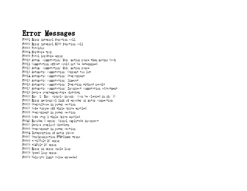
Error MessagesF9001 Error internal function call.F9002 Error internal RTOS function callF9003 WatchdogF9004 Hardware trapF8000 Fatal hardware errorF8010 Autom. commutation: Max. motion range when moving back F8011 Commutation offset could not be determinedF8012 Autom. commutation: Max. motion rangeF8013 Automatic commutation: Current too lowF8014 Automatic commutation: OvercurrentF8015 Automatic commutation: TimeoutF8016 Automatic commutation: Iteration without resultF8017 Automatic commutation: Incorrect commutation adjustment F8018 Device overtemperature shutdownF8022 Enc. 1: Enc. signals incorr. (can be cleared in ph. 2) F8023 Error mechanical link of encoder or motor connectionF8025 Overvoltage in power sectionF8027 Safe torque off while drive enabledF8028 Overcurrent in power sectionF8030 Safe stop 1 while drive enabledF8042 Encoder 2 error: Signal amplitude incorrectF8057 Device overload shutdownF8060 Overcurrent in power sectionF8064 Interruption of motor phaseF8067 Synchronization PWM-Timer wrongF8069 +/-15Volt DC errorF8070 +24Volt DC errorF8076 Error in error angle loopF8078 Speed loop error.F8079 Velocity limit value exceededF8091 Power section defectiveF8100 Error when initializing the parameter handlingF8102 Error when initializing power sectionF8118 Invalid power section/firmware combinationF8120 Invalid control section/firmware combinationF8122 Control section defectiveF8129 Incorrect optional module firmwareF8130 Firmware of option 2 of safety technology defectiveF8133 Error when checking interrupting circuitsF8134 SBS: Fatal errorF8135 SMD: Velocity exceededF8140 Fatal CCD error.F8201 Safety command for basic initialization incorrectF8203 Safety technology configuration parameter invalidF8813 Connection error mains chokeF8830 Power section errorF8838 Overcurrent external braking resistorF7010 Safely-limited increment exceededF7011 Safely-monitored position, exceeded in pos. DirectionF7012 Safely-monitored position, exceeded in neg. DirectionF7013 Safely-limited speed exceededF7020 Safe maximum speed exceededF7021 Safely-limited position exceededF7030 Position window Safe stop 2 exceededF7031 Incorrect direction of motionF7040 Validation error parameterized - effective thresholdF7041 Actual position value validation errorF7042 Validation error of safe operation modeF7043 Error of output stage interlockF7050 Time for stopping process exceeded8.3.15 F7051 Safely-monitored deceleration exceeded (159)8.4 Travel Range Errors (F6xxx) (161)8.4.1 Behavior in the Case of Travel Range Errors (161)8.4.2 F6010 PLC Runtime Error (162)8.4.3 F6024 Maximum braking time exceeded (163)8.4.4 F6028 Position limit value exceeded (overflow) (164)8.4.5 F6029 Positive position limit exceeded (164)8.4.6 F6030 Negative position limit exceeded (165)8.4.7 F6034 Emergency-Stop (166)8.4.8 F6042 Both travel range limit switches activated (167)8.4.9 F6043 Positive travel range limit switch activated (167)8.4.10 F6044 Negative travel range limit switch activated (168)8.4.11 F6140 CCD slave error (emergency halt) (169)8.5 Interface Errors (F4xxx) (169)8.5.1 Behavior in the Case of Interface Errors (169)8.5.2 F4001 Sync telegram failure (170)8.5.3 F4002 RTD telegram failure (171)8.5.4 F4003 Invalid communication phase shutdown (172)8.5.5 F4004 Error during phase progression (172)8.5.6 F4005 Error during phase regression (173)8.5.7 F4006 Phase switching without ready signal (173)8.5.8 F4009 Bus failure (173)8.5.9 F4012 Incorrect I/O length (175)8.5.10 F4016 PLC double real-time channel failure (176)8.5.11 F4017 S-III: Incorrect sequence during phase switch (176)8.5.12 F4034 Emergency-Stop (177)8.5.13 F4140 CCD communication error (178)8.6 Non-Fatal Safety Technology Errors (F3xxx) (178)8.6.1 Behavior in the Case of Non-Fatal Safety Technology Errors (178)8.6.2 F3111 Refer. missing when selecting safety related end pos (179)8.6.3 F3112 Safe reference missing (179)8.6.4 F3115 Brake check time interval exceeded (181)Troubleshooting Guide | Rexroth IndraDrive Electric Drivesand ControlsI Bosch Rexroth AG VII/XXIITable of ContentsPage8.6.5 F3116 Nominal load torque of holding system exceeded (182)8.6.6 F3117 Actual position values validation error (182)8.6.7 F3122 SBS: System error (183)8.6.8 F3123 SBS: Brake check missing (184)8.6.9 F3130 Error when checking input signals (185)8.6.10 F3131 Error when checking acknowledgment signal (185)8.6.11 F3132 Error when checking diagnostic output signal (186)8.6.12 F3133 Error when checking interrupting circuits (187)8.6.13 F3134 Dynamization time interval incorrect (188)8.6.14 F3135 Dynamization pulse width incorrect (189)8.6.15 F3140 Safety parameters validation error (192)8.6.16 F3141 Selection validation error (192)8.6.17 F3142 Activation time of enabling control exceeded (193)8.6.18 F3143 Safety command for clearing errors incorrect (194)8.6.19 F3144 Incorrect safety configuration (195)8.6.20 F3145 Error when unlocking the safety door (196)8.6.21 F3146 System error channel 2 (197)8.6.22 F3147 System error channel 1 (198)8.6.23 F3150 Safety command for system start incorrect (199)8.6.24 F3151 Safety command for system halt incorrect (200)8.6.25 F3152 Incorrect backup of safety technology data (201)8.6.26 F3160 Communication error of safe communication (202)8.7 Non-Fatal Errors (F2xxx) (202)8.7.1 Behavior in the Case of Non-Fatal Errors (202)8.7.2 F2002 Encoder assignment not allowed for synchronization (203)8.7.3 F2003 Motion step skipped (203)8.7.4 F2004 Error in MotionProfile (204)8.7.5 F2005 Cam table invalid (205)8.7.6 F2006 MMC was removed (206)8.7.7 F2007 Switching to non-initialized operation mode (206)8.7.8 F2008 RL The motor type has changed (207)8.7.9 F2009 PL Load parameter default values (208)8.7.10 F2010 Error when initializing digital I/O (-> S-0-0423) (209)8.7.11 F2011 PLC - Error no. 1 (210)8.7.12 F2012 PLC - Error no. 2 (210)8.7.13 F2013 PLC - Error no. 3 (211)8.7.14 F2014 PLC - Error no. 4 (211)8.7.15 F2018 Device overtemperature shutdown (211)8.7.16 F2019 Motor overtemperature shutdown (212)8.7.17 F2021 Motor temperature monitor defective (213)8.7.18 F2022 Device temperature monitor defective (214)8.7.19 F2025 Drive not ready for control (214)8.7.20 F2026 Undervoltage in power section (215)8.7.21 F2027 Excessive oscillation in DC bus (216)8.7.22 F2028 Excessive deviation (216)8.7.23 F2031 Encoder 1 error: Signal amplitude incorrect (217)VIII/XXII Bosch Rexroth AG | Electric Drivesand ControlsRexroth IndraDrive | Troubleshooting GuideTable of ContentsPage8.7.24 F2032 Validation error during commutation fine adjustment (217)8.7.25 F2033 External power supply X10 error (218)8.7.26 F2036 Excessive position feedback difference (219)8.7.27 F2037 Excessive position command difference (220)8.7.28 F2039 Maximum acceleration exceeded (220)8.7.29 F2040 Device overtemperature 2 shutdown (221)8.7.30 F2042 Encoder 2: Encoder signals incorrect (222)8.7.31 F2043 Measuring encoder: Encoder signals incorrect (222)8.7.32 F2044 External power supply X15 error (223)8.7.33 F2048 Low battery voltage (224)8.7.34 F2050 Overflow of target position preset memory (225)8.7.35 F2051 No sequential block in target position preset memory (225)8.7.36 F2053 Incr. encoder emulator: Pulse frequency too high (226)8.7.37 F2054 Incr. encoder emulator: Hardware error (226)8.7.38 F2055 External power supply dig. I/O error (227)8.7.39 F2057 Target position out of travel range (227)8.7.40 F2058 Internal overflow by positioning input (228)8.7.41 F2059 Incorrect command value direction when positioning (229)8.7.42 F2063 Internal overflow master axis generator (230)8.7.43 F2064 Incorrect cmd value direction master axis generator (230)8.7.44 F2067 Synchronization to master communication incorrect (231)8.7.45 F2068 Brake error (231)8.7.46 F2069 Error when releasing the motor holding brake (232)8.7.47 F2074 Actual pos. value 1 outside absolute encoder window (232)8.7.48 F2075 Actual pos. value 2 outside absolute encoder window (233)8.7.49 F2076 Actual pos. value 3 outside absolute encoder window (234)8.7.50 F2077 Current measurement trim wrong (235)8.7.51 F2086 Error supply module (236)8.7.52 F2087 Module group communication error (236)8.7.53 F2100 Incorrect access to command value memory (237)8.7.54 F2101 It was impossible to address MMC (237)8.7.55 F2102 It was impossible to address I2C memory (238)8.7.56 F2103 It was impossible to address EnDat memory (238)8.7.57 F2104 Commutation offset invalid (239)8.7.58 F2105 It was impossible to address Hiperface memory (239)8.7.59 F2110 Error in non-cyclical data communic. of power section (240)8.7.60 F2120 MMC: Defective or missing, replace (240)8.7.61 F2121 MMC: Incorrect data or file, create correctly (241)8.7.62 F2122 MMC: Incorrect IBF file, correct it (241)8.7.63 F2123 Retain data backup impossible (242)8.7.64 F2124 MMC: Saving too slowly, replace (243)8.7.65 F2130 Error comfort control panel (243)8.7.66 F2140 CCD slave error (243)8.7.67 F2150 MLD motion function block error (244)8.7.68 F2174 Loss of motor encoder reference (244)8.7.69 F2175 Loss of optional encoder reference (245)Troubleshooting Guide | Rexroth IndraDrive Electric Drivesand Controls| Bosch Rexroth AG IX/XXIITable of ContentsPage8.7.70 F2176 Loss of measuring encoder reference (246)8.7.71 F2177 Modulo limitation error of motor encoder (246)8.7.72 F2178 Modulo limitation error of optional encoder (247)8.7.73 F2179 Modulo limitation error of measuring encoder (247)8.7.74 F2190 Incorrect Ethernet configuration (248)8.7.75 F2260 Command current limit shutoff (249)8.7.76 F2270 Analog input 1 or 2, wire break (249)8.7.77 F2802 PLL is not synchronized (250)8.7.78 F2814 Undervoltage in mains (250)8.7.79 F2815 Overvoltage in mains (251)8.7.80 F2816 Softstart fault power supply unit (251)8.7.81 F2817 Overvoltage in power section (251)8.7.82 F2818 Phase failure (252)8.7.83 F2819 Mains failure (253)8.7.84 F2820 Braking resistor overload (253)8.7.85 F2821 Error in control of braking resistor (254)8.7.86 F2825 Switch-on threshold braking resistor too low (255)8.7.87 F2833 Ground fault in motor line (255)8.7.88 F2834 Contactor control error (256)8.7.89 F2835 Mains contactor wiring error (256)8.7.90 F2836 DC bus balancing monitor error (257)8.7.91 F2837 Contactor monitoring error (257)8.7.92 F2840 Error supply shutdown (257)8.7.93 F2860 Overcurrent in mains-side power section (258)8.7.94 F2890 Invalid device code (259)8.7.95 F2891 Incorrect interrupt timing (259)8.7.96 F2892 Hardware variant not supported (259)8.8 SERCOS Error Codes / Error Messages of Serial Communication (259)9 Warnings (Exxxx) (263)9.1 Fatal Warnings (E8xxx) (263)9.1.1 Behavior in the Case of Fatal Warnings (263)9.1.2 E8025 Overvoltage in power section (263)9.1.3 E8026 Undervoltage in power section (264)9.1.4 E8027 Safe torque off while drive enabled (265)9.1.5 E8028 Overcurrent in power section (265)9.1.6 E8029 Positive position limit exceeded (266)9.1.7 E8030 Negative position limit exceeded (267)9.1.8 E8034 Emergency-Stop (268)9.1.9 E8040 Torque/force actual value limit active (268)9.1.10 E8041 Current limit active (269)9.1.11 E8042 Both travel range limit switches activated (269)9.1.12 E8043 Positive travel range limit switch activated (270)9.1.13 E8044 Negative travel range limit switch activated (271)9.1.14 E8055 Motor overload, current limit active (271)9.1.15 E8057 Device overload, current limit active (272)X/XXII Bosch Rexroth AG | Electric Drivesand ControlsRexroth IndraDrive | Troubleshooting GuideTable of ContentsPage9.1.16 E8058 Drive system not ready for operation (273)9.1.17 E8260 Torque/force command value limit active (273)9.1.18 E8802 PLL is not synchronized (274)9.1.19 E8814 Undervoltage in mains (275)9.1.20 E8815 Overvoltage in mains (275)9.1.21 E8818 Phase failure (276)9.1.22 E8819 Mains failure (276)9.2 Warnings of Category E4xxx (277)9.2.1 E4001 Double MST failure shutdown (277)9.2.2 E4002 Double MDT failure shutdown (278)9.2.3 E4005 No command value input via master communication (279)9.2.4 E4007 SERCOS III: Consumer connection failed (280)9.2.5 E4008 Invalid addressing command value data container A (280)9.2.6 E4009 Invalid addressing actual value data container A (281)9.2.7 E4010 Slave not scanned or address 0 (281)9.2.8 E4012 Maximum number of CCD slaves exceeded (282)9.2.9 E4013 Incorrect CCD addressing (282)9.2.10 E4014 Incorrect phase switch of CCD slaves (283)9.3 Possible Warnings When Operating Safety Technology (E3xxx) (283)9.3.1 Behavior in Case a Safety Technology Warning Occurs (283)9.3.2 E3100 Error when checking input signals (284)9.3.3 E3101 Error when checking acknowledgment signal (284)9.3.4 E3102 Actual position values validation error (285)9.3.5 E3103 Dynamization failed (285)9.3.6 E3104 Safety parameters validation error (286)9.3.7 E3105 Validation error of safe operation mode (286)9.3.8 E3106 System error safety technology (287)9.3.9 E3107 Safe reference missing (287)9.3.10 E3108 Safely-monitored deceleration exceeded (288)9.3.11 E3110 Time interval of forced dynamization exceeded (289)9.3.12 E3115 Prewarning, end of brake check time interval (289)9.3.13 E3116 Nominal load torque of holding system reached (290)9.4 Non-Fatal Warnings (E2xxx) (290)9.4.1 Behavior in Case a Non-Fatal Warning Occurs (290)9.4.2 E2010 Position control with encoder 2 not possible (291)9.4.3 E2011 PLC - Warning no. 1 (291)9.4.4 E2012 PLC - Warning no. 2 (291)9.4.5 E2013 PLC - Warning no. 3 (292)9.4.6 E2014 PLC - Warning no. 4 (292)9.4.7 E2021 Motor temperature outside of measuring range (292)9.4.8 E2026 Undervoltage in power section (293)9.4.9 E2040 Device overtemperature 2 prewarning (294)9.4.10 E2047 Interpolation velocity = 0 (294)9.4.11 E2048 Interpolation acceleration = 0 (295)9.4.12 E2049 Positioning velocity >= limit value (296)9.4.13 E2050 Device overtemp. Prewarning (297)Troubleshooting Guide | Rexroth IndraDrive Electric Drivesand Controls| Bosch Rexroth AG XI/XXIITable of ContentsPage9.4.14 E2051 Motor overtemp. prewarning (298)9.4.15 E2053 Target position out of travel range (298)9.4.16 E2054 Not homed (300)9.4.17 E2055 Feedrate override S-0-0108 = 0 (300)9.4.18 E2056 Torque limit = 0 (301)9.4.19 E2058 Selected positioning block has not been programmed (302)9.4.20 E2059 Velocity command value limit active (302)9.4.21 E2061 Device overload prewarning (303)9.4.22 E2063 Velocity command value > limit value (304)9.4.23 E2064 Target position out of num. range (304)9.4.24 E2069 Holding brake torque too low (305)9.4.25 E2070 Acceleration limit active (306)9.4.26 E2074 Encoder 1: Encoder signals disturbed (306)9.4.27 E2075 Encoder 2: Encoder signals disturbed (307)9.4.28 E2076 Measuring encoder: Encoder signals disturbed (308)9.4.29 E2077 Absolute encoder monitoring, motor encoder (encoder alarm) (308)9.4.30 E2078 Absolute encoder monitoring, opt. encoder (encoder alarm) (309)9.4.31 E2079 Absolute enc. monitoring, measuring encoder (encoder alarm) (309)9.4.32 E2086 Prewarning supply module overload (310)9.4.33 E2092 Internal synchronization defective (310)9.4.34 E2100 Positioning velocity of master axis generator too high (311)9.4.35 E2101 Acceleration of master axis generator is zero (312)9.4.36 E2140 CCD error at node (312)9.4.37 E2270 Analog input 1 or 2, wire break (312)9.4.38 E2802 HW control of braking resistor (313)9.4.39 E2810 Drive system not ready for operation (314)9.4.40 E2814 Undervoltage in mains (314)9.4.41 E2816 Undervoltage in power section (314)9.4.42 E2818 Phase failure (315)9.4.43 E2819 Mains failure (315)9.4.44 E2820 Braking resistor overload prewarning (316)9.4.45 E2829 Not ready for power on (316)。
基站告警代码分析与处理RBS2000系列(RBS2202、RBS2301、RBS2302、RBS2206)1 1 SO CF,external condition map class 1故障代码:SO CF EC1:4故障名称:L/R SWI(BTS in local mode)故障原因:DXU处在local本地模式,BSC失去对其的控制。
故障处理:按DXU上的Local/remote按钮,使DXU进入remote远端模式。
故障代码:SO CF EC1:5故障名称:L/R TI(Local to remote while link lost)故障原因:当DXU正在由Local状态转换为remote状态时,传输中断,导致告警产生。
故障处理:在保证传输正常的情况下,对DXU进行复位。
2 2 SO CF,external condition map class 2故障代码:SO CF EC2:10故障名称:Mails fail(External power source fail)说明:适用R8A软件版本故障原因:对PSU的直流或交流供电存在断路等问题故障处理:检查如下方面:● 基站交流是否停电● -48V PSU的直流输入开关是否跳脱● 230V交流PSU的交流输入开关是否跳脱● ACCU故障,或连接错误(仅对室外型基站)故障代码:SO CF EC2:11故障名称:ALNA/TMA fault说明:适用于R8A软件版本相关故障:AO RX I1B:1 — ALNA/TMA fault故障原因:TMA塔顶放大器可能存在故障。
使用TMA的RX接收通路获得较弱的接收信号,相当于减少了3.5dB的灵敏度。
如果其它接收边也出现故障,会导致告警AO RX I1B:1的产生。
TMA的电流消耗可被CDU监测,可通过OMT进行监控。
当TMA的电流超出范围33-147mA,此告警产生。
TMA的电流值门限可以通过OMT在IDB中设臵。
A non-local algorithm for image denoisingAntoni Buades,Bartomeu Coll Dpt.Matem`a tiques i Inform`a tica,UIB Ctra.Valldemossa Km.7.5,07122Palma de Mallorca,Spain vdmiabc4@uib.es,tomeu.coll@uib.esJean-Michel MorelCMLA,ENS Cachan 61,Av du Pr´e sident Wilson 94235Cachan,France morel@cmla.ens-cachan.frAbstractWe propose a new measure,the method noise,to evalu-ate and compare the performance of digital image denois-ing methods.Wefirst compute and analyze this method noise for a wide class of denoising algorithms,namely the local smoothingfilters.Second,we propose a new algo-rithm,the non local means(NL-means),based on a non lo-cal averaging of all pixels in the image.Finally,we present some experiments comparing the NL-means algorithm and the local smoothingfilters.1.IntroductionThe goal of image denoising methods is to recover the original image from a noisy measurement,v(i)=u(i)+n(i),(1) where v(i)is the observed value,u(i)is the“true”value and n(i)is the noise perturbation at a pixel i.The best simple way to model the effect of noise on a digital image is to add a gaussian white noise.In that case,n(i)are i.i.d.gaussian values with zero mean and varianceσ2.Several methods have been proposed to remove the noise and recover the true image u.Even though they may be very different in tools it must be emphasized that a wide class share the same basic remark:denoising is achieved by ave-raging.This averaging may be performed locally:the Gaus-sian smoothing model(Gabor[7]),the anisotropicfiltering (Perona-Malik[11],Alvarez et al.[1])and the neighbor-hoodfiltering(Yaroslavsky[16],Smith et al.[14],Tomasi et al.[15]),by the calculus of variations:the Total Varia-tion minimization(Rudin-Osher-Fatemi[13]),or in the fre-quency domain:the empirical Wienerfilters(Yaroslavsky [16])and wavelet thresholding methods(Coiffman-Donoho [5,4]).Formally we define a denoising method D h as a decom-positionv=D h v+n(D h,v),where v is the noisy image and h is afiltering parame-ter which usually depends on the standard deviation of the noise.Ideally,D h v is smoother than v and n(D h,v)looks like the realization of a white noise.The decomposition of an image between a smooth part and a non smooth or oscillatory part is a current subject of research(for example Osher et al.[10]).In[8],Y.Meyer studied the suitable func-tional spaces for this decomposition.The primary scope of this latter study is not denoising since the oscillatory part contains both noise and texture.The denoising methods should not alter the original im-age u.Now,most denoising methods degrade or remove the fine details and texture of u.In order to better understand this removal,we shall introduce and analyze the method noise.The method noise is defined as the difference be-tween the original(always slightly noisy)image u and its denoised version.We also propose and analyze the NL-means algorithm, which is defined by the simple formulaNL[u](x)=1C(x)Ωe−(G a∗|u(x+.)−u(y+.)|2)(0)h2u(y)dy, where x∈Ω,C(x)=Ωe−(G a∗|u(x+.)−u(z+.)|2)(0)h2dz is a normalizing constant,G a is a Gaussian kernel and h acts as afiltering parameter.This formula amounts to say that the denoised value at x is a mean of the values of all points whose gaussian neighborhood looks like the neighborhood of x.The main difference of the NL-means algorithm with respect to localfilters or frequency domainfilters is the sys-tematic use of all possible self-predictions the image can provide,in the spirit of[6].For a more detailed analysis on the NL-means algorithm and a more complete comparison, see[2].Section2introduces the method noise and computes its mathematical formulation for the mentioned local smooth-ingfilters.Section3gives a discrete definition of the NL-means algorithm.In section4we give a theoretical result on the consistency of the method.Finally,in section5we compare the performance of the NL-means algorithm and the local smoothingfilters.2.Method noiseDefinition1(Method noise)Let u be an image and D h a denoising operator depending on afiltering parameter h. Then,we define the method noise as the image differenceu−D h u.The application of a denoising algorithm should not al-ter the non noisy images.So the method noise should be very small when some kind of regularity for the image is assumed.If a denoising method performs well,the method noise must look like a noise even with non noisy images and should contain as little structure as possible.Since even good quality images have some noise,it makes sense to evaluate any denoising method in that way,without the traditional“add noise and then remove it”trick.We shall list formulas permitting to compute and analyze the method noise for several classical local smoothingfilters:the Gaus-sianfiltering[7],the anisotropicfiltering[1,11],the Total Variation minimization[13]and the neighborhoodfiltering [16].The formal analysis of the method noise for the fre-quency domainfilters fall out of the scope of this paper. These method noises can also be computed but their inter-pretation depends on the particular choice of the wavelet basis.2.1.The GaussianfilteringThe image isotropic linearfiltering boils down to the convolution of the image by a linear symmetric kernel.The paradigm of such kernels is of course the gaussian kernelx→G h(x)=1(4πh2)e−|x|24h2.In that case,G h has standarddeviation h and it is easily seen thatTheorem1(Gabor1960)The image method noise of the convolution with a gaussian kernel G h isu−G h∗u=−h2∆u+o(h2),for h small enough.The gaussian method noise is zero in harmonic parts of the image and very large near edges or texture,where the Laplacian cannot be small.As a consequence,the Gaussian convolution is optimal inflat parts of the image but edges and texture are blurred.2.2.The anisotropicfilteringThe anisotropicfilter(A F)attempts to avoid the blurring effect of the Gaussian by convolving the image u at x only in the direction orthogonal to Du(x).The idea of suchfilter goes back to Perona and Malik[11].It is defined byA F h u(x)=G h(t)u(x+tDu(x)⊥|Du(x)|)dt,for x such that Du(x)=0and where(x,y)⊥=(−y,x) and G h is the one-dimensional Gauss function with vari-ance h2.If one assumes that the original image u is twice continuously differentiable(C2)at x,it is easily shown by a second order Taylor expansion thatTheorem2The image method noise of an anisotropicfilter A F h isu(x)−A F h u(x)=−12h2|Du|curv(u)(x)+o(h2),where the relation holds when Du(x)=0.By curv(u)(x),we denote the curvature,i.e.the signed inverse of the radius of curvature of the level line passing by x.This method noise is zero wherever u behaves locally like a straight line and large in curved edges or texture(where the curvature and gradient operators take high values).As a consequence,the straight edges are well restored whileflat and textured regions are degraded.2.3.The Total Variation minimizationThe Total Variation minimization was introduced by Rudin,Osher and Fatemi[13].Given a noisy image v(x), these authors proposed to recover the original image u(x) as the solution of the minimization problemTVFλ(v)=arg minuT V(u)+λ|v(x)−u(x)|2d xwhere T V(u)denotes the total variation of u andλis a given Lagrange multiplier.The minimum of the above min-imization problem exists and is unique.The parameterλis related to the noise statistics and controls the degree of filtering of the obtained solution.Theorem3The method noise of the Total Variation mini-mization isu(x)−TVFλ(u)(x)=−12λcurv(TVFλ(u))(x).As in the anisotropic case,straight edges are maintained because of their small curvature.However,details and tex-ture can be over smoothed ifλis too small.2.4.The neighborhood filteringWe call neighborhood filter any filter which restores a pixel by taking an average of the values of neighboring pix-els with a similar grey level value.Yaroslavsky (1985)[16]averages pixels with a similar grey level value and belong-ing to the spatial neighborhood B ρ(x ),YNF h,ρu (x )=1C (x )B ρ(x )u (y )e −|u (y )−u (x )|2h 2d y ,(2)where x ∈Ω,C (x )= B ρ(x )e −|u (y )−u (x )|22d y is the normal-ization factor and h is a filtering parameter.The Yaroslavsky filter is less known than more recent versions,namely the SUSAN filter (1995)[14]and the Bilat-eral filter (1998)[15].Both algorithms,instead of consider-ing a fixed spatial neighborhood B ρ(x ),weigh the distance to the reference pixel x ,SNF h,ρu (x )=1C (x ) Ωu (y )e −|y −x |22e −|u (y )−u (x )|2h 2d y ,(3)where C (x )= Ωe −|y −x |22e −|u (y )−u (x )|2h 2d y is the normaliza-tion factor and ρis now a spatial filtering parameter.In prac-tice,there is no difference between YNF h,ρand SNF h,ρ.If the grey level difference between two regions is larger than h ,both algorithms compute averages of pixels belonging to the same region as the reference pixel.Thus,the algorithm does not blur the edges,which is its main scope.In the experimentation section we only compare the Yaroslavsky neighborhood filter.The problem with these filters is that comparing only grey level values in a single pixel is not so robust when these values are noisy.Neighborhood filters also create ar-tificial shocks which can be justified by the computation of its method noise,see [3].3.NL-means algorithmGiven a discrete noisy image v ={v (i )|i ∈I },the estimated value NL [v ](i ),for a pixel i ,is computed as a weighted average of all the pixels in the image,NL [v ](i )=j ∈Iw (i,j )v (j ),where the family of weights {w (i,j )}j depend on the si-milarity between the pixels i and j,and satisfy the usual conditions 0≤w (i,j )≤1and j w (i,j )=1.The similarity between two pixels i and j depends on the similarity of the intensity gray level vectors v (N i )and v (N j ),where N k denotes a square neighborhood of fixed size and centered at a pixel k .This similarity ismeasuredFigure 1.Scheme of NL-means strategy.Similar pixel neighborhoods give a large weight,w(p,q1)and w(p,q2),while much different neighborhoods give a small weight w(p,q3).as a decreasing function of the weighted Euclidean distance, v (N i )−v (N j ) 22,a ,where a >0is the standard deviation of the Gaussian kernel.The application of the Euclidean distance to the noisy neighborhoods raises the following equalityE ||v (N i )−v (N j )||22,a =||u (N i )−u (N j )||22,a +2σ2.This equality shows the robustness of the algorithm since in expectation the Euclidean distance conserves the order of similarity between pixels.The pixels with a similar grey level neighborhood to v (N i )have larger weights in the average,see Figure 1.These weights are defined as,w (i,j )=1Z (i )e −||v (N i )−v (N j )||22,a2,where Z (i )is the normalizing constantZ (i )=je−||v (N i )−v (N i )||22,a2and the parameter h acts as a degree of filtering.It controls the decay of the exponential function and therefore the de-cay of the weights as a function of the Euclidean distances.The NL-means not only compares the grey level in a sin-gle point but the the geometrical configuration in a whole neighborhood.This fact allows a more robust comparison than neighborhood filters.Figure 1illustrates this fact,the pixel q 3has the same grey level value of pixel p ,but the neighborhoods are much different and therefore the weight w (p,q 3)is nearly zero.(a)(b)(c)(d)(e)(f)Figure2.Display of the NL-means weight distribution used to estimate the central pixel of every image.The weights go from1(white)to zero(black).4.NL-means consistencyUnder stationarity assumptions,for a pixel i,the NL-means algorithm converges to the conditional expectationof i once observed a neighborhood of it.In this case,thestationarity conditions amount to say that as the size of theimage grows we canfind many similar patches for all thedetails of the image.Let V be a randomfield and suppose that the noisy ima-ge v is a realization of V.Let Z denote the sequence ofrandom variables Z i={Y i,X i}where Y i=V(i)is realvalued and X i=V(N i\{i})is R p valued.The NL-meansis an estimator of the conditional expectation r(i)=E[Y i|X i=v(N i\{i})].Theorem4(Conditional expectation theorem)Let Z={V(i),V(N i\{i})}for i=1,2,...be a strictly sta-tionary and mixing process.Let NL n denote theNL-means algorithm applied to the sequence Z n={V(i),V(N i\{i})}n i=1.Then,|NL n(j)−r(j)|→0 a.sfor j∈{1,...,n}.The full statement of the hypothesis of the theorem and itsproof can be found in a more general framework in[12].This theorem tells us that the NL-means algorithm correctsthe noisy image rather than trying to separate the noise(os-cillatory)from the true image(smooth).In the case that an additive white noise model is assumed,the next result shows that the conditional expectation is thefunction of V(N i\{i})that minimizes the mean square er-ror with the true image u.Theorem5Let V,U,N be randomfields on I such thatV=U+N,where N is a signal independent white noise.Then,the following statements are hold.(i)E[V(i)|X i=x]=E[U(i)|X i=x]for all i∈Iand x∈R p.(ii)The expected random variable E[U(i)|V(N i\{i})]is the function of V(N i\{i})that minimizes the meansquare errormingE[U(i)−g(V(N i\{i}))]2Similar optimality theoretical results have been obtained in[9]and presented for the denoising of binary images.Theo-retical links between the two algorithms will be explored ina future work.5.Discussion and experimentationIn this section we compare the local smoothingfiltersand the NL-means algorithm under three well defined cri-teria:the method noise,the visual quality of the restoredimage and the mean square error,that is,the Euclidean dif-ference between the restored and true images.For computational purposes of the NL-means algorithm,we can restrict the search of similar windows in a larger”search window”of size S×S pixels.In all the experimen-tation we havefixed a search window of21×21pixels and asimilarity square neighborhood N i of7×7pixels.If N2isthe number of pixels of the image,then thefinal complexityof the algorithm is about49×441×N2.The7×7similarity window has shown to be largeenough to be robust to noise and small enough to take careof details andfine structure.Thefiltering parameter h hasbeenfixed to10∗σwhen a noise of standard deviationσis added.Due to the fast decay of the exponential kernel,large Euclidean distances lead to nearly zero weights actingas an automatic threshold,see Fig.2.Figure3.Denoising experience on a natural texture.From left to right:noisy image(standard deviation35), Gaussfiltering,anisotropicfiltering,Total variation,Neighborhoodfiltering and NL-meansalgorithm.Figure4.Method noise experience on a natural image.Displaying of the image difference u−D h(u).From left to right and from top to bottom:original image,Gaussfiltering,anisotropicfiltering,Total variation minimization, Neighborhoodfiltering and NL-means algorithm.The visual experiments corroborate the formulas of section2.In section2we have computed explicitly the methodnoise of the local smoothingfilters.These formulas are cor-roborated by the visual experiments of Figure4.Thisfig-ure displays the method noise for the standard image Lena,that is,the difference u−D h(u),where the parameter h is beenfixed in order to remove a noise of standard devia-tion2.5.The method noise helps us to understand the per-formance and limitations of the denoising algorithms,sinceremoved details or texture have a large method noise.Wesee in Figure4that the NL-means method noise does notpresent any noticeable geometrical structures.Figure2ex-plains this property since it shows how the NL-means al-gorithm chooses a weighting configuration adapted to thelocal and non local geometry of the image.The human eye is the only one able to decide if thequality of the image has been improved by the denoisingmethod.We display some denoising experiences compar-ing the NL-means algorithm with local smoothingfilters.All experiments have been simulated by adding a gaussianwhite noise of standard deviationσto the true image.Theobjective is to compare the visual quality of the restoredimages,the non presence of artifacts and the correct recon-struction of edges,texture and details.Due to the nature of the algorithm,the most favorable case for the NL-means is the textured or periodic case.In this situation,for every pixel i,we canfind a large set of samples with a very similar configuration.See Figure2e) for an example of the weight distribution of the NL-means algorithm for a periodic image.Figure3compares the per-formance of the NL-means and local smoothingfilters for a natural texture.Natural images also have enough redundancy to be re-stored by NL-means.Flat zones present a huge number of similar configurations lying inside the same object,see Fig-ure2(a).Straight or curved edges have a complete line of pixels with similar configurations,see Figure2(b)and (c).In addition,natural images allow us tofind many simi-lar configurations in far away pixels,as Figure2(f)shows. Figure5shows an experiment on a natural image.This ex-perience must be compared with Figure4,where we display the method noise of the original image.The blurred or de-graded structures of the restored images coincide with the noticeable structures of its method noise.Finally Table1displays the mean square error for theFigure5.Denoising experience on a natural image.From left to right and from top to bottom:noisy image (standard deviation20),Gaussfiltering,anisotropicfiltering,Total variation,Neighborhoodfiltering and NL-means algorithm.The removed details must be compared with the method noise experience,Figure4.Image GF AF TVF YNF NLLena12011411012968Baboon507418365381292Table1.Mean square error table.A smaller meansquare error indicates that the estimate is closerto the original image.denoising experiments given in the paper.This numericalmeasurement is the most objective one,since it does notrely on any visual interpretation.However,this error is notcomputable in a real problem and a small mean square errordoes not assure a high visual quality.So all above discussedcriteria seem necessary to compare the performance of al-gorithms.References[1]L.Alvarez,P.-L.Lions,and J.-M.Morel.Image selectivesmoothing and edge detection by nonlinear diffusion(ii).Journal of numerical analysis,29:845–866,1992.[2] A.Buades,B.Coll,and J.Morel.On image denoising meth-ods.Technical Report2004-15,CMLA,2004.[3] A.Buades,B.Coll,and J.Morel.Neighborhoodfilters andpde’s.Technical Report2005-04,CMLA,2005.[4]R.Coifman and D.Donoho.Wavelets and Statistics,chapterTranslation-invariant de-noising,pages125–150.SpringerVerlag,1995.[5] D.Donoho.De-noising by soft-thresholding.IEEE Trans-actions on Information Theory,41:613–627,1995.[6] A.Efros and T.Leung.Texture synthesis by non parametricsampling.In puter Vision,volume2,pages1033–1038,1999.[7]M.Lindenbaum,M.Fischer,and A.Bruckstein.On gaborcontribution to image enhancement.Pattern Recognition,27:1–8,1994.[8]Y.Meyer.Oscillating Patterns in Image Processing andNonlinear Evolution Equations,volume22.AMS Univer-sity Lecture Series,2002.[9] E.Ordentlich,G.Seroussi,M.W.S.Verd´u,and T.Weiss-man.A discrete universal denoiser and its application to bi-nary images.In Proc.IEEE ICIP,volume1,pages117–120,2003.[10]S.Osher,A.Sole,and L.Vese.Image decomposition andrestoration using total variation minimization and the h−1norm.Multiscale Modeling and Simulation,1(3):349–370,2003.[11]P.Perona and J.Malik.Scale space and edge detection usinganisotropic diffusion.IEEE Trans.Patt.Anal.Mach.Intell.,12:629–639,1990.[12]G.Roussas.Nonparametric regression estimation undermixing conditions.Stochastic processes and their applica-tions,36:107–116,1990.[13]L.Rudin,S.Osher,and E.Fatemi.Nonlinear total variationbased noise removal algorithms.Physica D,60:259–268,1992.[14]S.Smith and J.Brady.Susan-a new approach to low levelimage processing.International Journal of Computer Vi-sion,23(1):45–78,1997.[15] C.Tomasi and R.Manduchi.Bilateralfiltering for gray andcolor images.In Proceedings of the Sixth Internatinal Con-ference on Computer Vision,pages839–846,1998.[16]L.Yaroslavsky.Digital Picture Processing-An Introduc-tion.Springer Verlag,1985.。
a r X i v :c o n d -m a t /0607011v 1 [c o n d -m a t .s t r -e l ] 1 J u l 2006Journal of Magnetism and Magnetic Materials 0(2008)1–0/locate/jmmmNonlocal Effect of Local Nonmagnetic Impurity in High-T c Superconductors:Induced Local Moment and Huge Residual ResistivityHiroshi Kontani a ,∗,Masanori Ohno aa Departmentof Physics,Nagoya University,Furo-cho,Nagoya 464-8602,Japan.Received May 2006;revised 2006;accepted 2006In under-doped high-T c superconductors (HTSC’s),nonmagnetic impurities (such as Zn)causes nontrivial widespread change of the electronic states.For example,both the local and the staggered spin susceptibilities are strongly enhanced around the impurity,within the ra-dius of the AF correlation length ξAF .This behavior was experimentally observed in the site-selective 89Y NMR measurements for Zn-doped YBCO [1].Moreover,a small concentration of Zn causes a huge residual resistivity,much beyond the s-wave unitary scattering limit [2].These non-trivial impurity effects had been frequently considered as the evidence of the breakdown of the Fermi liquid state in under-doped HTSC’s.Pure HTSC’s samples also show various intrinsic non-Fermi liquid (NFL)behaviors free from impurity effects.Many of them had been explained based on the spin fluc-tuation theories like the SCR theory and the fluctuation-exchange (FLEX)approximation [3].For example,Curie like behavior of the Hall coefficient R H is naturally under-stood if one take the current vertex correction (CVC)due to AF fluctuations into account [4].Anomalous transport phenomena in the pseudo-gap region,such as a drastic in-crement of the Nernst coefficient,are also reproduced by246810χs(r ,r )246χs(r ,r )(1,0)(5,0)(3,0)Fig.1.Local spin susceptibility obtained by the GV I -method around the impurity site (at (0,0)).the effective interaction given by the FLEX-type diagramscomposed of ˆGI =({ˆG 00}−1−ˆI −ˆΣ0)−1.That is,ˆG I =ˆG|δΣ=0.In the GV I -method,ˆG is solved self-consistently whereas ˆVI is a partially self-consistent function.As proved in ref.[6],GV I -method is much inferior to a fully self-consistent GV -method.Hereafter,we take the unitary limit I =∞.Numerical results of the spin susceptibility given by the GV I -method in site representation,χIs (r ,r ),are explained in Ref.[6].Here,we present the local susceptibility χIs (r ,r )in Fig.1,around the impurity site (at (0,0))along the x -direction.Here,we put (t,t ′,t ′′)=(−1,1/6,−1/5),where t ′,t ′,and t ′′are the nearest,the next nearest,and the third nearest neighbor hopping integrals,respectively.We assume U =8for hole-doped system (YBCO)and U =5.5for electron-doped system (NCCO).T =0.02corresponds to 80K in real systems.At r =(7,0),χIs (r ,r )takes almost an bulk value without impurity.However,it increases gradually as one approach the impurity.The temperature dependence of χIs (r ,r )away from the impurity is moderate.On the other hand,it increases drastically around the impurity as temperature decreases.At the same time,the radius of the enlargement of χIs (r ,r )increases.The obtained result is highly consistent with NMR measurements [1].Here,we discuss the physical reason for the obtained im-purity effect.In the FLEX approximation,the AF-order (in the RPA)is suppressed by thermal and quantum fluc-tuations.In the GV I -method,the reduction of fluctuationsT12ρFig.2.Temperature dependence of ρfor NCCO with dilute impuritiesgiven by the GV I -method.due to an impurity gives rise to the enhancement of sus-ceptibility.However,this mechanism is absent in the RPA.Therefore,the enhancement of susceptibility is tiny within the RPA.Next,we discuss the transport phenomena in the pres-ence of dilute impurities on the basis of the GV I -method [6].Figure 2shows the resistivity ρfor NCCO with n imp =0,0.01and 0.02.The obtained result shows a huge parallel shift of resistivity at finite temperatures (∆ρ)due to im-purities,far beyond the s-wave unitary scattering limit.As T decreases,nonmagnetic impurities cause a “Kondo-like upturn”of ρbelow T x ,reflecting an extremely short quasi-particle lifetime around the impurities.We see that T x de-creases as n imp does.The obtained Kondo-like upturn of ρstrongly suggests that the insulating behavior of ρobserved in under-doped HTSC’s is caused by residual disorder in the CuO 2-plane,or residual apical oxygen in NCCO.The present study reveals that a single impurity strongly affects the electronic states in a wide area around the im-purity in the vicinity of the AF-QCP.Here,we developed the GV I -FLEX method,which is a powerful method to study the impurity effect in strongly correlated ing the GV I method,characteristic impurity effects in under-doped HTSC’s are well explained in a unified way,without introducing any exotic mechanisms which assume the breakdown of the Fermi liquid state.Qualita-tively,these obtained numerical results are very similar for YBCO,LSCO and NCCO.We succeeds in explaining nontrivial impurity effects in HTSC’s in a unified way in terms of a spin fluctuation theory,which strongly suggests that the ground state of HTSC is a Fermi liquid.We expect that novel impurity effects in other metals near AF-QCP,such as heavy fermion systems and organic metals,could be explained by the GV I -method.References[1] A.V.Mahajan et al.,Eur.Phy.J.B 13(2000)457.[2]Y.Fukuzumi et al.,Phys.Rev.Lett.76(1996)684.[3]H.Kontani and K.Yamada,J.Phy.Soc.Jpn.74(2005),p.155.[4]H.Kontani,K.Kanki and K.Ueda,Phys.Rev.B59(1999)p.14723.[5]H.Kontani,Phys.Rev.Lett.89(2003)237003.[6]H.Kontani and M.Ohno,Phys.Rev.B(2006).。