计量经济学第四章习题详解
- 格式:docx
- 大小:195.56 KB
- 文档页数:10
(2) 3.060 1.657ln() 1.057ln()
(0.337) (0.092) (0.215)0.992 0.991 F 1275.093
GDP CPI R =-+-===进口居民消费价格指数的回归系数的符号不能进行合理的经济意义解释可能数据中有多重共线性。
计算相关系数:
22ln Y 4.09071.2186ln () t= (-10.6458) (34.6222)
0.9828 0.9820 1198.698
GDP R R F =-+===ln Y 5.4424 2.6637ln (PI)C =-+
从修正的可决系数和F统计量可以看出,全部变量对数线性多元回归整体对样本拟合很好,著。
可是其中的lnX3、lnX4、lnX6对lnY影响不显著,而且lnX2、lnX5
可以看出lnx1与lnx2、lnx3、lnx4、lnx5、lnx6之间高度相关,许多相关系数高于作为解释变量,很可能会出现严重多重共线性问题。
在本章开始的“引子”提出的“农业的发展反而会减少财政收入吗?
表4.13 1978-2007
财政收入(亿元)CS农业增加值(亿元)NZ工业增加值(亿元)GZ建筑业增加值
1132.31027.51607
1146.41270.21769.7
1159.91371.61996.5
1175.81559.52048.4
(1)根据样本数据得到各解释变量的样本相关系数矩阵如下:样本相关系数矩阵
解释变量之间相关系数较高,特别是农业增加值、工业增加值、建筑业增加值、最终消费之间,相关系数都在这显然与第三章对模型的无多重共线性假定不符合。

《计量经济学》习题(第四章)第四章习题⼀、单选题1、如果回归模型违背了同⽅差假定,最⼩⼆乘估计量____A .⽆偏的,⾮有效的 B.有偏的,⾮有效的C .⽆偏的,有效的 D.有偏的,有效的2、Goldfeld-Quandt ⽅法⽤于检验____A .异⽅差性 B.⾃相关性C .随机解释变量 D.多重共线性3、DW 检验⽅法⽤于检验____A .异⽅差性 B.⾃相关性C .随机解释变量 D.多重共线性4、在异⽅差性情况下,常⽤的估计⽅法是____A .⼀阶差分法 B.⼴义差分法C .⼯具变量法 D.加权最⼩⼆乘法5、在以下选项中,正确表达了序列⾃相关的是____j i u x Cov D j i x x Cov C ji u u Cov B ji u u Cov A j i j i j i j i ≠≠≠≠≠=≠≠,0),(.,0),(.,0),(.,0),(.6、如果回归模型违背了⽆⾃相关假定,最⼩⼆乘估计量____A .⽆偏的,⾮有效的 B.有偏的,⾮有效的C .⽆偏的,有效的 D.有偏的,有效的7、在⾃相关情况下,常⽤的估计⽅法____A .普通最⼩⼆乘法 B.⼴义差分法C .⼯具变量法 D.加权最⼩⼆乘法8、White 检验⽅法主要⽤于检验____A .异⽅差性 B.⾃相关性C .随机解释变量 D.多重共线性9、Glejser 检验⽅法主要⽤于检验____A .异⽅差性 B.⾃相关性C .随机解释变量 D.多重共线性10、简单相关系数矩阵⽅法主要⽤于检验____A .异⽅差性 B.⾃相关性C .随机解释变量 D.多重共线性2222)(.)(.)(.)(.σσσσ==≠≠i i i i x Var D u Var C x Var B u Var A12、所谓不完全多重共线性是指存在不全为零的数k λλλ,,,21 ,有____1112211221221122.0.0..k k k k k x x x k k k k A x x x v B x x x C x x x v e D x x x v e v λλλλλλλλλλλλ++++=+++=∑?++++=++++=式中是随机误差项13、设21,x x 为解释变量,则完全多重共线性是____0.(021.0.021.22121121=+=++==+x x e x D v v x x C e x B x x A 为随机误差项)14、⼴义差分法是对____⽤最⼩⼆乘法估计其参数 11211211121121)()1(....-------+-+-=-++=++=++=t t t t t t t t t t t t t t t u u x x y y D u x y C u x y B u x y A ρρβρβρρρβρβρββββ15、在DW 检验中要求有假定条件,在下列条件中不正确的是____A .解释变量为⾮随机的 B.随机误差项为⼀阶⾃回归形式C .线性回归模型中不应含有滞后内⽣变量为解释变量D.线性回归模型为⼀元回归形式16、在下例引起序列⾃相关的原因中,不正确的是____A.经济变量具有惯性作⽤B.经济⾏为的滞后性C.设定偏误D.解释变量之间的共线性17、在DW 检验中,当d 统计量为2时,表明____A.存在完全的正⾃相关B.存在完全的负⾃相关C.不存在⾃相关D.不能判定18、在DW 检验中,当d 统计量为4时,表明____A.存在完全的正⾃相关B.存在完全的负⾃相关C.不存在⾃相关D.不能判定19、在DW 检验中,当d 统计量为0时,表明____A.存在完全的正⾃相关C.不存在⾃相关D.不能判定20、在DW 检验中,存在不能判定的区域是____A. 0﹤d ﹤l d ,4-l d ﹤d ﹤4B. u d ﹤d ﹤4-u dC. l d ﹤d ﹤u d ,4-u d ﹤d ﹤4-l dD. 上述都不对21、在修正序列⾃相关的⽅法中,能修正⾼阶⾃相关的⽅法是____A. 利⽤DW 统计量值求出ρB. Cochrane-Orcutt 法C. Durbin 两步法D. 移动平均法22、在下列多重共线性产⽣的原因中,不正确的是____A.经济本变量⼤多存在共同变化趋势B.模型中⼤量采⽤滞后变量C.由于认识上的局限使得选择变量不当D.解释变量与随机误差项相关23、在DW 检验中,存在正⾃相关的区域是____A. 4-l d ﹤d ﹤4B. 0﹤d ﹤l dC. u d ﹤d ﹤4-u dD. l d ﹤d ﹤u d ,4-u d ﹤d ﹤4-l d24、逐步回归法既检验⼜修正了____A .异⽅差性 B.⾃相关性 C .随机解释变量 D.多重共线性25、设)()(,2221i i i i i ix f u Var u x y σσββ==++=,则对原模型变换的正确形式为____ )()()()(.)()()()(.)()()()(..212222122121i i i i i i i i i i i i i i i i i i i i i i i i x f u x f x x f x f y D x f u x f x x f x f y C x f u x f x x f x f y B u x y A ++=++=++=++=ββββββββ 26、在修正序列⾃相关的⽅法中,不正确的是____A.⼴义差分法B.普通最⼩⼆乘法C.⼀阶差分法D. Durbin 两步法27、在检验异⽅差的⽅法中,不正确的是____A. Goldfeld-Quandt ⽅法B. spearman 检验法C. White 检验法28、在DW 检验中,存在零⾃相关的区域是____A. 4-l d ﹤d ﹤4B. 0﹤d ﹤l dC. u d ﹤d ﹤4-u dD. l d ﹤d ﹤u d ,4-u d ﹤d ﹤4-l d29.如果模型中的解释变量存在完全的多重共线性,参数的最⼩⼆乘估计量是()A .⽆偏的 B. 有偏的 C. 不确定 D. 确定的30. 已知模型的形式为u x y 21+β+β=,在⽤实际数据对模型的参数进⾏估计的时候,测得DW 统计量为0.6453,则⼴义差分变量是( )A. 1t t ,1t t x 6453.0x y 6453.0y ----B. 1t t 1t t x 6774.0x ,y 6774.0y ----C. 1t t 1t t x x ,y y ----D. 1t t 1t t x 05.0x ,y 05.0y ----31. 在具体运⽤加权最⼩⼆乘法时,如果变换的结果是x u x x x 1xy 21+β+β=,则Var(u)是下列形式中的哪⼀种?( )A. 2σxB. 2σ2x B. 2σx D. 2σLog(x)32. 在线性回归模型中,若解释变量1x 和2x 的观测值成⽐例,即有i 2i 1kx x =,其中k 为⾮零常数,则表明模型中存在( )A. 异⽅差B. 多重共线性C. 序列⾃相关D. 设定误差33. 已知DW 统计量的值接近于2,则样本回归模型残差的⼀阶⾃相关系数ρ近似等于( ) A. 0 B. –1 C. 1 D. 4⼆、多项选择1、能够检验多重共线性的⽅法有____A.简单相关系数法B. DW检验法C. 判定系数检验法D. ⽅差膨胀因⼦检验E.逐步回归法2、能够修正多重共线性的⽅法有____A.增加样本容量B.岭回归法C.剔除多余变量E.差分模型3、如果模型中存在异⽅差现象,则会引起如下后果____A. 参数估计值有偏B. 参数估计值的⽅差不能正确确定C. 变量的显著性检验失效D. 预测精度降低E. 参数估计值仍是⽆偏的4、能够检验异⽅差的⽅法是____A. gleiser检验法B. White检验法C. 图形法D. spearman检验法E. DW检验法F. Goldfeld-Quandt检验法5、如果模型中存在序列⾃相关现象,则会引起如下后果____A. 参数估计值有偏B. 参数估计值的⽅差不能正确确定C. 变量的显著性检验失效D. 预测精度降低E. 参数估计值仍是⽆偏的6、检验序列⾃相关的⽅法是____A. gleiser检验法B. White检验法C. 图形法D. DW检验法E. Goldfeld-Quandt检验法7、能够修正序列⾃相关的⽅法有____A. 加权最⼩⼆乘法B. Durbin两步法C. ⼴义最⼩⼆乘法D. ⼀阶差分法E. ⼴义差分法8、Goldfeld-Quandt检验法的应⽤条件是____A. 将观测值按解释变量的⼤⼩顺序排列B. 样本容量尽可能⼤C. 随机误差项服从正态分布D. 将排列在中间的约1/4的观测值删除掉9、在DW检验中,存在不能判定的区域是____A. 0﹤d﹤l dB. u d﹤d﹤4-u dC. l d﹤d﹤u dD. 4-u d﹤d﹤4-l dE. 4-l d﹤d﹤4。
第四章习题4.1没有进行t 检验,并且调整的可决系数也没有写出来,也就是没有考虑自由度的影响,会使结果存在一研究的目的和要求我们知道,商品进口额与很多因素有关,了解其变化对进出口产品有很大帮助。
为了探究和预测商品 进口额的变化,需要定量地分析影响商品进口额变化的主要因素。
二、模型的设定及其估计经分析,商品进口额可能与国内生产总值、居民消费价格指数有关。
为此,考虑国内生产总值 居民消费价格指数 CPI 为主要因素。
各影响变量与商品进口额呈正相关。
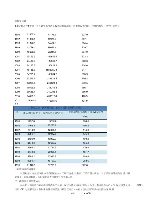
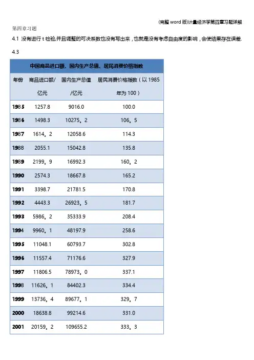
为此,设定如下形式的计量经济 模型:4.3199511048.160793.7302.8+ In+ InCP1996 11557.4 71176.6 327.9 1997 11806.5 78973.0 337.1 1998 11626.1 84402.3 334.4 1999 13736.4 89677.1 329.7 2000 18638.8 99214.6 331.0 2001 20159.2 109655.2 333.3 2002 24430.3 120332.7 330.6 2003 34195.6 135822.8 334.6 2004 46435.8 159878.3 I 347.7 2005 54273.7 183084.8 353.9 2006 63376.9 211923.5 359.2 2007 73284.6 249529.9 376.5 2008 79526.5 314045.4 398.7 2009 68618.4 340902.8 395.9 201094699.3 401512.8 408.9 2011113161.4472881.6431.0GDP 、式中, 为第 年中国商品进口额(亿元);In GDP 为第 年国内生产总值(亿元);In CPI 为居民消费价格 指数(以1985年为100)。
各解释变量前的回归系数预期都大于零。
第四章习题4.1 没有进行t检验,并且调整的可决系数也没有写出来,也就是没有考虑自由度的影响,会使结果存在误差.4.3200224430.3120332。
7 330.6200334195。
6135822.8 334。
6200446435.8159878.3 l347.7200554273.7183084.8 353.9200663376.9211923。
5 359。
2200773284。
6249529。
9 376.5200879526.5314045.4 398.7200968618。
4340902。
8 395。
9201094699.3401512.8 408。
92011113161.4472881.6 431.0一研究的目的和要求我们知道,商品进口额与很多因素有关,了解其变化对进出口产品有很大帮助。
为了探究和预测商品进口额的变化,需要定量地分析影响商品进口额变化的主要因素。
二、模型的设定及其估计经分析,商品进口额可能与国内生产总值、居民消费价格指数有关。
为此,考虑国内生产总值GDP、居民消费价格指数CPI为主要因素。
各影响变量与商品进口额呈正相关。
为此,设定如下形式的计量经济模型:=+ln+lnCP式中,亿元);lnGDP为国内生产总值(亿元);lnCPI为居民消费价格指数(以1985年为100)。
各解释变量前的回归系数预期都大于零。
为估计模型,根据上表的数据,利用EViews软件,生成Y、lnGDP、lnCPI等数据,采用OLS方法估计模型参数,得到的回归结果如下图所示:模型方程为:lnY=-3。
111486+1。
338533lnGDP-0.421791lnCPI(0。
463010)(0。
088610)(0。
233295)t= (—6。
720126) (15。
10582)(—1。
807975)=0.988051 =0.987055 F=992。
2582该模型=0.988051,=0。
987055,可决系数很高,F检验值为992.2582,明显显著。
第四章练习题及参考解答4.1 假设在模型i i i iu X X Y +++=33221βββ中,32X X 与之间的相关系数为零,于是有人建议你进行如下回归:ii i i i i u X Y u X Y 23311221++=++=γγαα(1)是否存在3322ˆˆˆˆβγβα==且?为什么? (2)111ˆˆˆβαγ会等于或或两者的某个线性组合吗? (3)是否有()()()()3322ˆvar ˆvar ˆvar ˆvarγβαβ==且? 练习题4.1参考解答:(1) 存在3322ˆˆˆˆβγβα==且。
因为()()()()()()()23223223232322ˆ∑∑∑∑∑∑∑--=iiiii iii iii x x x x x xx y x x y β当32X X 与之间的相关系数为零时,离差形式的032=∑i i x x有()()()()222223222322ˆˆαβ===∑∑∑∑∑∑iiiiiiii xx y x x x x y 同理有:33ˆˆβγ= (2) 111ˆˆˆβαγ会等于或的某个线性组合 因为12233ˆˆˆY X X βββ=--,且122ˆˆY X αα=-,133ˆˆY X γγ=- 由于3322ˆˆˆˆβγβα==且,则 11222222ˆˆˆˆˆY Y X Y X X αααββ-=-=-=11333333ˆˆˆˆˆY Y X Y X X γγγββ-=-=-=则 1112233231123ˆˆˆˆˆˆˆY Y Y X X Y X X Y X X αγβββαγ--=--=--=+- (3) 存在()()()()3322ˆvar ˆvar ˆvar ˆvarγβαβ==且。
因为()()∑-=22322221ˆvarr x iσβ当023=r 时,()()()22222232222ˆvar 1ˆvar ασσβ==-=∑∑iixr x 同理,有()()33ˆvar ˆvar γβ=4.2在决定一个回归模型的“最优”解释变量集时人们常用逐步回归的方法。

计量经济学课后答案第四、五章(内容参考)第四章随机解释变量问题1. 随机解释变量的来源有哪些?答:随机解释变量的来源有:经济变量的不可控,使得解释变量观测值具有随机性;由于随机干扰项中包括了模型略去的解释变量,而略去的解释变量与模型中的解释变量往往是相关的;模型中含有被解释变量的滞后项,而被解释变量本身就是随机的。
2.随机解释变量有几种情形? 分情形说明随机解释变量对最小二乘估计的影响与后果?答:随机解释变量有三种情形,不同情形下最小二乘估计的影响和后果也不同。
(1)解释变量是随机的,但与随机干扰项不相关;这时采用OLS估计得到的参数估计量仍为无偏估计量;(2)解释变量与随机干扰项同期无关、不同期相关;这时OLS估计得到的参数估计量是有偏但一致的估计量;(3)解释变量与随机干扰项同期相关;这时OLS估计得到的参数估计量是有偏且非一致的估计量。
3. 选择作为工具变量的变量必须满足那些条件?答:选择作为工具变量的变量需满足以下三个条件:(1)与所替代的随机解释变量高度相关;(2)与随机干扰项不相关;(3)与模型中其他解释变量不相关,以避免出现多重共线性。
4.对模型Y t =β+β1X1t+β2X2t+β3Yt-1+μt假设Yt-1与μt相关。
为了消除该相关性,采用工具变量法:先求Y t关于X1t与 X2t回归,得到Yt,再做如下回归:Y t =β+β1X1t+β2X2t+β3Y t?1-+μt试问:这一方法能否消除原模型中Yt的相关性? 为什么?解答:能消除。
在基本假设下,X1t,X2t与μt应是不相关的,由此知,由X1t 与X2t估计出的Yt应与μt不相关。
5.对于一元回归模型Y t =β+β1Xt*+μt假设解释变量Xt *的实测值Xt与之有偏误:Xt= Xt*+et,其中et是具有零均值、无序列相关,且与Xt不相关的随机变量。
试问:(1) 能否将X t= X t*+e t代入原模型,使之变换成Y t=β0+β1X t+νt后进行估计? 其中,νt为变换后模型的随机干扰项。
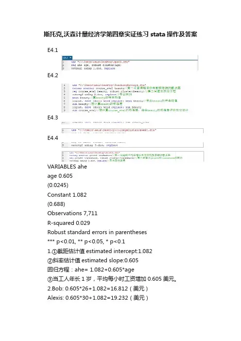
斯托克,沃森计量经济学第四章实证练习stata操作及答案E4.1E4.2E4.3E4.4VARIABLES aheage 0.605(0.0245)Constant 1.082(0.688)Observations 7,711R-squared 0.029Robust standard errors in parentheses*** p<0.01, ** p<0.05, * p<0.11.①截距估计值estimated intercept:1.082②斜率估计值estimated slope:0.605回归方程:ahe= 1.082+0.605*age③当工人年长1岁,平均每小时工资增加0.605美元。
2.Bob: 0.605*26+1.082=16.812(美元)Alexis: 0.605*30+1.082=19.232(美元)答:预测Bob的收入为每小时16.812美元,Alexis为19.232美元。
3.年龄不能解释不同个体收入变化的大部分。
因为R-squared反映了因变量的全部变化能通过回归关系被自变量充分解释的比例,而分析得R-squared的值为0.029,解释度低,说明年龄不能解释不同个体收入变化的大部分。
1.答:两者看上去有微弱的正相关关系2.VARIABLES course_evalbeauty 0.133(0.0550)Constant 3.998(0.0449)Observations 463R-squared 0.036Robust standard errors in parentheses*** p<0.01, ** p<0.05, * p<0.1①截距估计值:3.998斜率估计值:0.133回归方程:Course_Eval=3.998+0.133*beauty//mean beautyMean estimation Number of obs = 463Mean Std.Err. 95% Conf. Interval beauty 4.75e-08 0.0367 -0.0720 0.0720②截距的估计值=Course_Eval的样本均值-斜率估计值*Beauty 的样本均值计算得Beauty的样本均值趋近于零,所以截距的估计值等于Course_Eval的样本均值。
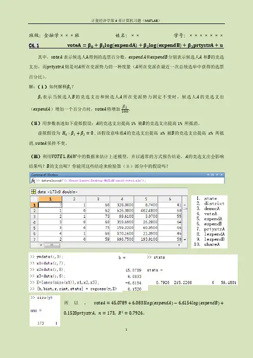
班级:金融学×××班姓名:××学号:×××××××C4.1 voteA=β0+β1log expendA+β2log expendB+β3prtystrA+u 其中,voteA表示候选人A得到的选票百分数,expendA和expendB分别表示候选人A和B的竞选支出,而prtystrA则是对A所在党派势力的一种度量(A所在党派在最近一次总统选举中获得的选票百分比)。
解:(ⅰ)如何解释β1?β1表示当候选人B的竞选支出和候选人A所在党派势力固定不变时,候选人A的竞选支出(expendA)增加一个百分点时,voteA将增加β1 100。
(ⅱ)用参数表述如下虚拟假设:A的竞选支出提高1% 被B的竞选支出提高1% 所抵消。
虚拟假设为H0∶β1+β2=0 ,该假设意味着A的竞选支出提高x% 被B的竞选支出提高x% 所抵消,voteA保持不变。
(ⅲ)利用VOTE1.RAW中的数据来估计上述模型,并以通常的方式报告结论。
A的竞选支出会影响结果吗?B的支出呢?你能用这些结论来检验第(ⅱ)部分中的假设吗?所以,voteA=45.0789+6.0833log expendA−6.6154log expendB+0.1520prtystrA, n=173, R2=0.7926 .由截图可得:expendA 系数β1的 t 统计量为15.9187,在很小的显著水平上都是显著的,意味着当其他条件不变时,A 的竞选支出增加1%,voteA 将增加0.0608。
同理可得,expendB 系数β2的 t 统计量为-17.4632,在很小的显著水平上都是显著的,意味着当其他条件不变时,B 的竞选支出增加1%,voteA 将增加0.066。
由于A 的竞选支出的系数β1和B 的竞选支出的系数β2符号相反,绝对值差不多,所以近似有虚拟假设“ H 0∶β1+β2=0 ”成立,即第(ⅱ)部分中的假设成立。
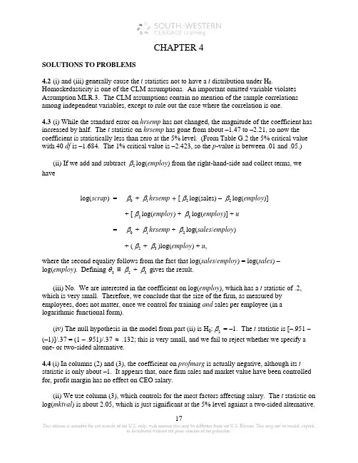
17CHAPTER 4SOLUTIONS TO PROBLEMS4.2 (i) and (iii) generally cause the t statistics not to have a t distribution under H 0.Homoskedasticity is one of the CLM assumptions. An important omitted variable violates Assumption MLR.3. The CLM assumptions contain no mention of the sample correlations among independent variables, except to rule out the case where the correlation is one.4.3 (i) While the standard error on hrsemp has not changed, the magnitude of the coefficient has increased by half. The t statistic on hrsemp has gone from about –1.47 to –2.21, so now the coefficient is statistically less than zero at the 5% level. (From Table G.2 the 5% critical value with 40 df is –1.684. The 1% critical value is –2.423, so the p -value is between .01 and .05.)(ii) If we add and subtract 2βlog(employ ) from the right-hand-side and collect terms, we havelog(scrap ) = 0β + 1βhrsemp + [2βlog(sales) – 2βlog(employ )] + [2βlog(employ ) + 3βlog(employ )] + u = 0β + 1βhrsemp + 2βlog(sales /employ ) + (2β + 3β)log(employ ) + u ,where the second equality follows from the fact that log(sales /employ ) = log(sales ) – log(employ ). Defining 3θ ≡ 2β + 3β gives the result.(iii) No. We are interested in the coefficient on log(employ ), which has a t statistic of .2, which is very small. Therefore, we conclude that the size of the firm, as measured by employees, does not matter, once we control for training and sales per employee (in a logarithmic functional form).(iv) The null hypothesis in the model from part (ii) is H 0:2β = –1. The t statistic is [–.951 – (–1)]/.37 = (1 – .951)/.37 ≈ .132; this is very small, and we fail to reject whether we specify a one- or two-sided alternative.4.4 (i) In columns (2) and (3), the coefficient on profmarg is actually negative, although its t statistic is only about –1. It appears that, once firm sales and market value have been controlled for, profit margin has no effect on CEO salary.(ii) We use column (3), which controls for the most factors affecting salary. The t statistic on log(mktval ) is about 2.05, which is just significant at the 5% level against a two-sided alternative.18(We can use the standard normal critical value, 1.96.) So log(mktval ) is statistically significant. Because the coefficient is an elasticity, a ceteris paribus 10% increase in market value is predicted to increase salary by 1%. This is not a huge effect, but it is not negligible, either.(iii) These variables are individually significant at low significance levels, with t ceoten ≈ 3.11 and t comten ≈ –2.79. Other factors fixed, another year as CEO with the company increases salary by about 1.71%. On the other hand, another year with the company, but not as CEO, lowers salary by about .92%. This second finding at first seems surprising, but could be related to the “superstar” effect: firms that hire CEOs from outside the company often go after a small pool of highly regarded candidates, and salaries of these people are bid up. More non-CEO years with a company makes it less likely the person was hired as an outside superstar.4.7 (i) .412 ± 1.96(.094), or about .228 to .596.(ii) No, because the value .4 is well inside the 95% CI.(iii) Yes, because 1 is well outside the 95% CI.4.8 (i) With df = 706 – 4 = 702, we use the standard normal critical value (df = ∞ in Table G.2), which is 1.96 for a two-tailed test at the 5% level. Now t educ = −11.13/5.88 ≈ −1.89, so |t educ | = 1.89 < 1.96, and we fail to reject H 0: educ β = 0 at the 5% level. Also, t age ≈ 1.52, so age is also statistically insignificant at the 5% level.(ii) We need to compute the R -squared form of the F statistic for joint significance. But F = [(.113 − .103)/(1 − .113)](702/2) ≈ 3.96. The 5% critical value in the F 2,702 distribution can be obtained from Table G.3b with denominator df = ∞: cv = 3.00. Therefore, educ and age are jointly significant at the 5% level (3.96 > 3.00). In fact, the p -value is about .019, and so educ and age are jointly significant at the 2% level.(iii) Not really. These variables are jointly significant, but including them only changes the coefficient on totwrk from –.151 to –.148.(iv) The standard t and F statistics that we used assume homoskedasticity, in addition to the other CLM assumptions. If there is heteroskedasticity in the equation, the tests are no longer valid.4.11 (i) Holding profmarg fixed, n rdintensΔ = .321 Δlog(sales ) = (.321/100)[100log()sales ⋅Δ] ≈ .00321(%Δsales ). Therefore, if %Δsales = 10, n rdintens Δ ≈ .032, or only about 3/100 of a percentage point. For such a large percentage increase in sales,this seems like a practically small effect.(ii) H 0:1β = 0 versus H 1:1β > 0, where 1β is the population slope on log(sales ). The t statistic is .321/.216 ≈ 1.486. The 5% critical value for a one-tailed test, with df = 32 – 3 = 29, is obtained from Table G.2 as 1.699; so we cannot reject H 0 at the 5% level. But the 10% criticalvalue is 1.311; since the t statistic is above this value, we reject H0 in favor of H1 at the 10% level.(iii) Not really. Its t statistic is only 1.087, which is well below even the 10% critical value for a one-tailed test.1920SOLUTIONS TO COMPUTER EXERCISESC4.1 (i) Holding other factors fixed,111log()(/100)[100log()](/100)(%),voteA expendA expendA expendA βββΔ=Δ=⋅Δ≈Δwhere we use the fact that 100log()expendA ⋅Δ ≈ %expendA Δ. So 1β/100 is the (ceteris paribus) percentage point change in voteA when expendA increases by one percent.(ii) The null hypothesis is H 0: 2β = –1β, which means a z% increase in expenditure by A and a z% increase in expenditure by B leaves voteA unchanged. We can equivalently write H 0: 1β + 2β = 0.(iii) The estimated equation (with standard errors in parentheses below estimates) isn voteA = 45.08 + 6.083 log(expendA ) – 6.615 log(expendB ) + .152 prtystrA(3.93) (0.382) (0.379) (.062) n = 173, R 2 = .793.The coefficient on log(expendA ) is very significant (t statistic ≈ 15.92), as is the coefficient on log(expendB ) (t statistic ≈ –17.45). The estimates imply that a 10% ceteris paribus increase in spending by candidate A increases the predicted share of the vote going to A by about .61percentage points. [Recall that, holding other factors fixed, n voteAΔ≈(6.083/100)%ΔexpendA ).] Similarly, a 10% ceteris paribus increase in spending by B reduces n voteAby about .66 percentage points. These effects certainly cannot be ignored.While the coefficients on log(expendA ) and log(expendB ) are of similar magnitudes (andopposite in sign, as we expect), we do not have the standard error of 1ˆβ + 2ˆβ, which is what we would need to test the hypothesis from part (ii).(iv) Write 1θ = 1β +2β, or 1β = 1θ– 2β. Plugging this into the original equation, and rearranging, givesn voteA = 0β + 1θlog(expendA ) + 2β[log(expendB ) – log(expendA )] +3βprtystrA + u ,When we estimate this equation we obtain 1θ≈ –.532 and se( 1θ)≈ .533. The t statistic for the hypothesis in part (ii) is –.532/.533 ≈ –1. Therefore, we fail to reject H 0: 2β = –1β.21C4.3 (i) The estimated model isn log()price = 11.67 + .000379 sqrft + .0289 bdrms (0.10) (.000043) (.0296)n = 88, R 2 = .588.Therefore, 1ˆθ= 150(.000379) + .0289 = .0858, which means that an additional 150 square foot bedroom increases the predicted price by about 8.6%.(ii) 2β= 1θ – 1501β, and solog(price ) = 0β+ 1βsqrft + (1θ – 1501β)bdrms + u= 0β+ 1β(sqrft – 150 bdrms ) + 1θbdrms + u .(iii) From part (ii), we run the regressionlog(price ) on (sqrft – 150 bdrms ), bdrms ,and obtain the standard error on bdrms . We already know that 1ˆθ= .0858; now we also getse(1ˆθ) = .0268. The 95% confidence interval reported by my software package is .0326 to .1390(or about 3.3% to 13.9%).C4.5 (i) If we drop rbisyr the estimated equation becomesn log()salary = 11.02 + .0677 years + .0158 gamesyr (0.27) (.0121) (.0016)+ .0014 bavg + .0359 hrunsyr (.0011) (.0072)n = 353, R 2= .625.Now hrunsyr is very statistically significant (t statistic ≈ 4.99), and its coefficient has increased by about two and one-half times.(ii) The equation with runsyr , fldperc , and sbasesyr added is22n log()salary = 10.41 + .0700 years + .0079 gamesyr(2.00) (.0120) (.0027)+ .00053 bavg + .0232 hrunsyr (.00110) (.0086)+ .0174 runsyr + .0010 fldperc – .0064 sbasesyr (.0051) (.0020) (.0052) n = 353, R 2 = .639.Of the three additional independent variables, only runsyr is statistically significant (t statistic = .0174/.0051 ≈ 3.41). The estimate implies that one more run per year, other factors fixed,increases predicted salary by about 1.74%, a substantial increase. The stolen bases variable even has the “wrong” sign with a t statistic of about –1.23, while fldperc has a t statistic of only .5. Most major league baseball players are pretty good fielders; in fact, the smallest fldperc is 800 (which means .800). With relatively little variation in fldperc , it is perhaps not surprising that its effect is hard to estimate.(iii) From their t statistics, bavg , fldperc , and sbasesyr are individually insignificant. The F statistic for their joint significance (with 3 and 345 df ) is about .69 with p -value ≈ .56. Therefore, these variables are jointly very insignificant.C4.7 (i) The minimum value is 0, the maximum is 99, and the average is about 56.16. (ii) When phsrank is added to (4.26), we get the following:n log() wage = 1.459 − .0093 jc + .0755 totcoll + .0049 exper + .00030 phsrank (0.024) (.0070) (.0026) (.0002) (.00024)n = 6,763, R 2 = .223So phsrank has a t statistic equal to only 1.25; it is not statistically significant. If we increase phsrank by 10, log(wage ) is predicted to increase by (.0003)10 = .003. This implies a .3% increase in wage , which seems a modest increase given a 10 percentage point increase in phsrank . (However, the sample standard deviation of phsrank is about 24.)(iii) Adding phsrank makes the t statistic on jc even smaller in absolute value, about 1.33, but the coefficient magnitude is similar to (4.26). Therefore, the base point remains unchanged: the return to a junior college is estimated to be somewhat smaller, but the difference is not significant and standard significant levels.(iv) The variable id is just a worker identification number, which should be randomly assigned (at least roughly). Therefore, id should not be correlated with any variable in the regression equation. It should be insignificant when added to (4.17) or (4.26). In fact, its t statistic is about .54.23C4.9 (i) The results from the OLS regression, with standard errors in parentheses, aren log() psoda =−1.46 + .073 prpblck + .137 log(income ) + .380 prppov (0.29) (.031) (.027) (.133)n = 401, R 2 = .087The p -value for testing H 0: 10β= against the two-sided alternative is about .018, so that we reject H 0 at the 5% level but not at the 1% level.(ii) The correlation is about −.84, indicating a strong degree of multicollinearity. Yet eachcoefficient is very statistically significant: the t statistic for log()ˆincome β is about 5.1 and that forˆprppovβ is about 2.86 (two-sided p -value = .004).(iii) The OLS regression results when log(hseval ) is added aren log() psoda =−.84 + .098 prpblck − .053 log(income ) (.29) (.029) (.038) + .052 prppov + .121 log(hseval ) (.134) (.018)n = 401, R 2 = .184The coefficient on log(hseval ) is an elasticity: a one percent increase in housing value, holding the other variables fixed, increases the predicted price by about .12 percent. The two-sided p -value is zero to three decimal places.(iv) Adding log(hseval ) makes log(income ) and prppov individually insignificant (at even the 15% significance level against a two-sided alternative for log(income ), and prppov is does not have a t statistic even close to one in absolute value). Nevertheless, they are jointly significant at the 5% level because the outcome of the F 2,396 statistic is about 3.52 with p -value = .030. All of the control variables – log(income ), prppov , and log(hseval ) – are highly correlated, so it is not surprising that some are individually insignificant.(v) Because the regression in (iii) contains the most controls, log(hseval ) is individually significant, and log(income ) and prppov are jointly significant, (iii) seems the most reliable. It holds fixed three measure of income and affluence. Therefore, a reasonable estimate is that if the proportion of blacks increases by .10, psoda is estimated to increase by 1%, other factors held fixed.。
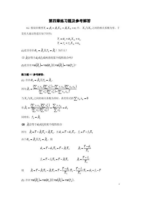
第四章练习题及参考解答4.1 假设在模型i i i i u X X Y +++=33221βββ中,32X X 与之间的相关系数为零,于是有人建议你进行如下回归:ii i i i i u X Y u X Y 23311221++=++=γγαα(1)是否存在3322ˆˆˆˆβγβα==且?为什么? (2)111ˆˆˆβαγ会等于或或两者的某个线性组合吗? (3)是否有()()()()3322ˆvar ˆvar ˆvar ˆvar γβαβ==且?练习题4.1参考解答:(1) 存在3322ˆˆˆˆβγβα==且。
因为()()()()()()()23223223232322ˆ∑∑∑∑∑∑∑--=iiiii iii iii x x x x x x x y x x y β当32X X 与之间的相关系数为零时,离差形式的032=∑i ix x有()()()()222223222322ˆˆαβ===∑∑∑∑∑∑iiiiiiii xx y x x x x y 同理有:33ˆˆβγ= (2) 111ˆˆˆβαγ会等于或的某个线性组合 因为 12233ˆˆˆY X X βββ=--,且122ˆˆY X αα=-,133ˆˆY X γγ=- 由于3322ˆˆˆˆβγβα==且,则 11222222ˆˆˆˆˆY Y X Y X X αααββ-=-=-= 11333333ˆˆˆˆˆY Y X Y X X γγγββ-=-=-= 则 1112233231123ˆˆˆˆˆˆˆY Y Y X X Y X X Y X X αγβββαγ--=--=--=+- (3) 存在()()()()3322ˆvar ˆvar ˆvar ˆvar γβαβ==且。
因为()()∑-=22322221ˆvar r x iσβ当023=r 时,()()()22222232222ˆvar 1ˆvar ασσβ==-=∑∑iixr x 同理,有()()33ˆvar ˆvar γβ=4.2在决定一个回归模型的“最优”解释变量集时人们常用逐步回归的方法。
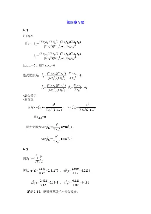
第四章习题4.1(1)存在因为:23223223232322-))(())((-))((ˆ)(ΣΣΣΣΣΣΣ=βi i i i i i i i i i i x x x x x x x y x x y 23223223222233-))(())((-))((ˆ)(ΣΣΣΣΣΣΣ=βi i i i i i i i i i i x x x x x x x y x x y 且032=x x r ,则032=Σi i x x 原式变形为:))(())((ˆ23222322i i i i i x x x x y ΣΣΣΣ=β=222ii i x x y ΣΣ=2αˆ ))(())((ˆ23222233i i i i i x x x x y ΣΣΣΣ=β=2333ˆi i i x x y ΣΣ=β=3αˆ (2)会等于(3)存在因为)r -1()ˆvar(i3i 22222i x Σσ=β, )r -1()ˆvar(i3i 23232i x Σσ=β 且032=x x r原式变形为2222)ˆvar(ix Σσ=β=)ˆvar(2α, 2323)ˆvar(i x Σσ=β=)ˆvar(3α 4.2因为 )ˆ(-ˆ111βββ=SE t 所以 t(c)=92.8133.8=0.91177 , 2294.60.171.059)ˆt(1==β 6848.00.660.452)ˆt(2==β , 111.01.090.121)ˆt(3==β R 2是0.95,说明模型对样本拟合较好。
F检验,F=107.37> F(3,23)=3.03,回归方程显著。
t检验,t统计量分别为0.91177,6.2294,0.6848,0.111,X2,X3对应的t 统计量绝对值均小于t(23)=2.069,X2,X3的系数不显著,可能存在多重共线性。
4.3(1)LnY=-3.111486+1.338533lnGDP-0.421791lnCPI(2)R2是0.988051,修正的R2为0.987055,说明模型对样本拟合较好。
计量经济学第四章作业思考题:4.3 多重共线性的典型表现是什么?判断是否存在多重共线性的方法有哪些?答:(1)多重共线性的典型表现:A.模型拟和较好,但偏回归系数几乎都无统计学意义;B.偏回归系数估计值不稳定,方差很大;C.偏回归系数估计值的符号可能与预期不符或与经验相悖,结果难以解释。
(2)具体的判断方法:A.解释变量之间简单相关系数矩阵法;B.方差扩大因子法;C.直观判断法;D.逐步回归的方法。
4.4 针对出现多重共线性的不同情形,能采取的补救措施有哪些?答:(1)根据经验,可以选择剔除变量,增大样本容量,变换模型形式,利用非样本先验信息,截面数据和时间序列数据并用以及变量变换等不同方法。
(2)采取逐步回归方法由由一元模型开始逐步增加解释变量个数,增加的原则是显著提高可决系数,自身显著而与其他变量之间又不产生共线性。
(3)采取岭回归方法来降低多重共线性的程度。
4.9 以下陈述是否正确?请判断并说明理由。
(1)在高度多重共线性的情形中,要评价一个或多个偏回归系数的单个显著性是不可能的。
答:正确。
(2)尽管有完全的多重共线性,OLS估计量仍然是BLUE。
答:错误。
(3)如果有某一辅助回归显示出高的R j2值,则高度共线性的存在肯定是无疑的。
答:正确。
(4)变量的两两高度相关并不表示高度多重共线性。
答:正确。
(5)如果其他条件不变,VIF越高,OLS估计量的方差越大。
答:正确。
(6)如果在多元回归中,根据通常的t检验,全部偏回归系数分别都是统计上不显著的,你就不会得到一个高的R2值。
答:错误。
(7)在Y对X2和X3的回归中,假如X3的值很少变化,这就会使Var(β3)增大,极端的情况下,如果全部X3值都相同,Var(β3) 将是无穷大。
答:正确。
(8)如果分析的目的仅仅是预测,则多重共线性是无害的。
答:错误。
练习题:4.3(1)利用eviews分析得到如下数据:Dependent Variable: LNYMethod: Least SquaresDate: 05/09/16 Time: 12:45Sample: 1985 2011Included observations: 27Variable Coefficient Std. Error t-Statistic Prob.C -3.111486 0.463010 -6.720126 0.0000LNGDP 1.338533 0.088610 15.10582 0.0000LNCPI -0.421791 0.233295 -1.807975 0.0832R-squared 0.988051 Mean dependent var 9.484710Adjusted R-squared 0.987055 S.D. dependent var 1.425517S.E. of regression 0.162189 Akaike info criterion -0.695670Sum squared resid 0.631326 Schwarz criterion -0.551689Log likelihood 12.39155 Hannan-Quinn criter. -0.652857F-statistic 992.2583 Durbin-Watson stat 0.522613Prob(F-statistic) 0.000000由上可知,模型为:lnY=1.338533lnGDP t—0.421791lnCPI t—3.111486(2)A.该模型的可决系数为0.988051,修正可决系数为0.987055,两者都很高。
第四章练习题及参考解答4.1 假设在模型i i i i u X X Y +++=33221βββ中,32X X 与之间的相关系数为零,有人建议你分别进行如下回归:1221i i i Y X u αα=++ 1332i i i Y X u γγ=++(1) 是否存在3322ˆˆˆˆβγβα==且?为什么? (2) 1ˆβ会等于1ˆα或1ˆγ或者两者的某个线性组合吗? (3) 是否有()()22ˆˆVar Var βα=且()()33ˆˆVar Var βγ=?【练习题4.1参考解答】(1) 存在2233ˆˆˆˆαβγβ==且 。
因为 ()()()()()()()22332322222323ˆi iii ii iiii iy x x y x x x x x x x β-=-∑∑∑∑∑∑∑当23X X 与 之间的相关系数为零时,离差形式的230i ix x =∑有 ()()()()223222222223ˆˆi i ii i iiiy x x y x xx x βα===∑∑∑∑∑∑ 同理有: 33ˆˆγβ= (2)会的。
(3) 存在 ()()()()2233ˆˆˆˆvar var var var βαβγ==且 因为 ()()2222223ˆvar 1ix r σβ=-∑当 230r = 时, ()()()22222222223ˆˆvar var 1iix x r σσβα===-∑∑ 同理,有 ()()33ˆˆvar var βγ=4.2 表4.4给出了1995—2016年中国商品进口额Y 、国生产总值GDP 、居民消费价格指数CPI 的数据。
表4.4 中国商品进口额、国生产总值、居民消费价格指数资料来源:《中国统计年鉴2017》考虑建立模型: i t t t u CPI GDP Y ++=ln ln ln 321βββ+ (1)利用表中数据估计此模型的参数。
(2)你认为数据中有多重共线性吗?(3)进行以下回归:121ln ln t t i Y A A GDP v =++ 122ln ln t t i Y B B CPI v =++ 123ln ln t t i GDP C C CPI v =++ 根据这些回归你能对多重共线性的性质有什么认识?(4)假设经检验数据有多重共线性,但模型中32ˆˆββ和在5%水平上显著,并且F 检验也显著,你对此模型的应用有何建议?【练习题4.2参考解答】建立模型: i t t t u CPI GDP Y ++=ln ln ln 321βββ+ (1)利用表中数据估计此模型的参数。
第三、四章习题09国贸1班张继云 1403.31)为分析家庭书刊年消费支出(Y)对家庭月平均收入(X)与户主受教育年数(T)的关系,做如图所示的线形图。
建立多元线性回归模型为Y i=β1+β2X+β3T+μi2) 假定所建立模型中的随机扰动项μi满足各项古典假设,用OLS法估计其参数,得到的回归结果如下。
可用规范形式将参数估计和检验结果写为Y = -50.01638+0.086450X+52.37031T(49.46026)(0.029363)(5.202167)t=(-1.011244)(2.944186)(10.06702)R2=0.951235 F=146.2974 n=183)对回归系数β3的t检验:针对H0:β3=0和H1:β3≠0,由回归结果中还可以看出,估计的回归系数β3的标准误差和t值分别为:SE(β3)= 5.202167, t(β3)= 10.6702。
当α=0.05时,查t分布表得自由度n-3=18-3=15的临界值t0.025(15)=2.131。
因为t(β1)= 10.6702> t0.025(16)=2.131,所以应该拒绝H0:β2=0。
这表明户主受教育年数对家庭书刊年消费支出有显著性影响。
4)所估计的模型的经济意义是当户主受教育年数保持不变时,家庭月平均收入每增加一元时将导致家庭书刊年消费支出增加0.086450元。
而当家庭月平均收入保持不变时,户主受教育年数每增加一年时将导致家庭书刊年消费支出增加52.37031元。
此模型可用于预测将来的家庭书刊年消费支出。
4.31)假定所建立模型中的随机扰动项μi满足各项古典假设,用OLS法估计其参数,得到的回归结果如下。
可用规范形式将参数估计和检验结果写为LnY t = -3.060638+1.056682lnGDP t-1.656536lnCPI t(0.337331)(0.092174) (0.214570)t = (-9.073096) (17.97182) (-4.924656)R2=0.992222 F=1275.739 n=232)数据中有多重共线性,居民消费价格指数的回归系数的符号不能进行合理的经济意义解释,且其简单相关系数呈现正向变动。
计量经济学练习题第一章导论一、单项选择题⒈计量经济研究中常用的数据主要有两类:一类是时间序列数据,另一类是【 B 】A 总量数据B 横截面数据C平均数据 D 相对数据⒉横截面数据是指【A 】A 同一时点上不同统计单位相同统计指标组成的数据B 同一时点上相同统计单位相同统计指标组成的数据C 同一时点上相同统计单位不同统计指标组成的数据D 同一时点上不同统计单位不同统计指标组成的数据⒊下面属于截面数据的是【D 】A 1991-2003年各年某地区20个乡镇的平均工业产值B 1991-2003年各年某地区20个乡镇的各镇工业产值C 某年某地区20个乡镇工业产值的合计数D 某年某地区20个乡镇各镇工业产值⒋同一统计指标按时间顺序记录的数据列称为【B 】A 横截面数据B 时间序列数据C 修匀数据D原始数据⒌回归分析中定义【 B 】A 解释变量和被解释变量都是随机变量B 解释变量为非随机变量,被解释变量为随机变量C 解释变量和被解释变量都是非随机变量D 解释变量为随机变量,被解释变量为非随机变量二、填空题⒈计量经济学是经济学的一个分支学科,是对经济问题进行定量实证研究的技术、方法和相关理论,可以理解为数学、统计学和_经济学_三者的结合。
⒉⒊现代计量经济学已经形成了包括单方程回归分析,联立方程组模型,时间序列分析三大支柱。
⒋⒌经典计量经济学的最基本方法是回归分析。
计量经济分析的基本步骤是:理论(或假说)陈述、建立计量经济模型、收集数据、计量经济模型参数的估计、检验和模型修正、预测和政策分析。
⒍⒎常用的三类样本数据是截面数据、时间序列数据和面板数据。
⒏⒐经济变量间的关系有不相关关系、相关关系、因果关系、相互影响关系和恒等关系。
三、简答题⒈什么是计量经济学?它与统计学的关系是怎样的?计量经济学就是对经济规律进行数量实证研究,包括预测、检验等多方面的工作。
计量经济学是一种定量分析,是以解释经济活动中客观存在的数量关系为内容的一门经济学学科。
第四章:多重共线性二、简答题1、导致多重共线性的原因有哪些?2、多重共线性为什么会使得模型的预测功能失效?3、如何利用辅回归模型来检验多重共线性?4、判断以下说法正确、错误,还是不确定?并简要陈述你的理由。
(1)尽管存在完全的多重共线性,OLS 估计量还是最优线性无偏估计量(BLUE )。
(2)在高度多重共线性的情况下,要评价一个或者多个偏回归系数的个别显著性是不可能的。
(3)如果某一辅回归显示出较高的2i R 值,则必然会存在高度的多重共线性。
(4)变量之间的相关系数较高是存在多重共线性的充分必要条件。
(5)如果回归的目的仅仅是为了预测,则变量之间存在多重共线性是无害的。
5、考虑下面的一组数据:12233i i i Y X X βββ=++来对以上数据进行拟合回归。
(1) 我们能得到这3个估计量吗?并说明理由。
(2) 如果不能,那么我们能否估计得到这些参数的线性组合?可以的话,写出必要的计算过程。
6、考虑以下模型:231234i i i i i Y X X X ββββμ=++++由于2X 和3X 是X 的函数,那么它们之间存在多重共线性。
这种说法对吗?为什么? 7、在涉及时间序列数据的回归分析中,如果回归模型不仅含有解释变量的当前值,同时还含有它们的滞后值,我们把这类模型称为分布滞后模型(distributed-lag model )。
我们考虑以下模型:12313233i t t t t t Y X X X X βββββμ---=+++++其中Y ——消费,X ——收入,t ——时间。
该模型表示当期的消费是其现期的收入及其滞后三期的收入的线性函数。
(1) 在这一类模型中是否会存在多重共线性?为什么? (2) 如果存在多重共线性的话,应该如何解决这个问题? 8、设想在模型12233i i i i Y X X βββμ=+++中,2X 和3X 之间的相关系数23r 为零。
如果我们做如下的回归:1221i i i Y X ααμ=++ 1332i i i Y X γγμ=++(1)会不会存在22ˆˆαβ=且33ˆˆγβ=?为什么? (2)1ˆβ会等于1ˆα或1ˆγ或两者的某个线性组合吗? (3)会不会有22ˆˆvar()var()βα=且33ˆˆvar()var()γβ=? 9、通过一些简单的计量软件(比如EViews 、SPSS ),我们可以得到各变量之间的相关矩阵:2323232311 1k k k k r r r r R r r ⎛⎫ ⎪ ⎪= ⎪ ⎪ ⎪⎝⎭。
第4章练习6解:(1)答:不能,因为将代入原模型中使其变换后的模型为,显然,由于与同期相关,则说明变换后的模型中的随机干扰项与同期相关。
解:(2)对于多数经济变量的时间序列,除非它们是以一阶差分的形式或变化率的形式出现,往往具有较强的相关性,因此,当和直接表示经济规模或水平的经济变量时,它们之间很可能相关;如果变量是一阶差分的形式或以变化率的形态出现,则它们间的相关性就会降低,但仍有一定程度的相关性。
解:(3)由(2)的结论知,,即与变换后的模型的随机干扰项不相关,而且与有较强的相关性,因此可用作为的工具变量对变换后的模型进行估计。
第4章练习10编编号号170080081006115018001876026501000100907120020002052039001200127308140022002201049501400142509155024002435051100160016930101500260026860解:根据eview软件操作得:Dependent Variable: YMethod: Least SquaresDate: 04/17/11 Time: 22:28Sample: 1 10Included observations: 10Variable CoefficientStd.Error t-Statistic Prob.C245.515869.523483.5314080.0096 X10.5684250.7160980.7937810.4534 X2-0.0058330.070294-0.0829750.9362R-squared0.962099 Mean dependentvar1110.000Adjusted R-squared0.951270 S.D. dependentvar314.2893S.E. ofregression69.37901 Akaike infocriterion11.56037Sum squaredresid33694.13 Schwarzcriterion11.65115Log likelihood-54.80185 Hannan-Quinncriter.11.46079F-statistic88.84545 Durbin-Watsonstat 2.708154Prob(F-statistic)0.000011根据以上表格可得估计的回归模型为:(3.53)(0.79)(-0.083)分析:1.从回归估计的结果看,模型拟合较好。
第四章习题
4.1 没有进行t检验,并且调整的可决系数也没有写出来,也就是没有考虑自由度的影响,会使结果存在误差。
一研究的目的和要求
我们知道,商品进口额与很多因素有关,了解其变化对进出口产品有很大帮助。
为了探究和预测商品进口额的变化,需要定量地分析影响商品进口额变化的主要因素。
二、模型的设定及其估计
经分析,商品进口额可能与国内生产总值、居民消费价格指数有关。
为此,考虑国内生产总值GDP、居民消费价格指数CPI为主要因素。
各影响变量与商品进口额呈正相关。
为此,设定如下形式的计量经济模型:
lnY t=β1+β2ln GDP t+β3lnCP I t
式中,Y t为第t年中国商品进口额(亿元);lnGDP为第t年国内生产总值(亿元);lnCPI为居民消费价格指数(以1985年为100)。
各解释变量前的回归系数预期都大于零。
为估计模型,根据上表的数据,利用EViews软件,生成Y、lnGDP、lnCPI等数据,采用OLS方法估计模型参数,得到的回归结果如下图所示:
模型方程为:
lnY=-3.111486+1.338533lnGDP-0.421791lnCPI
(0.463010) (0.088610) (0.233295)
t= (-6.720126) (15.10582) (-1.807975)
R2=0.988051 R̅2=0.987055 F=992.2582
该模型R2=0.988051,R̅2=0.987055,可决系数很高,F检验值为992.2582,明显显著。
但是当α=0.05 (n-k)=t0.025(27-3)=2.064,不仅lnCPI的系数不显著,而且,lnCPI的符号与预期相反,这表明可能存在时,tα
2
严重的多重共线性。
计算各解释变量的相关系数,选择lnGDP,lnCPI数据,“view/correlation”得相关系数矩阵。
1
由相关系数矩阵可以看出,各解释变量相互之间的相关系数较高,证实确实存在一定的多重共线性。
为了进一步了解多重共线性的性质,我们做辅助回归,即每个解释变量分别作为被解释变量都对剩余的解释变量进行回归。
lnGDP与lnCPI的相关系数很高,证明存在多重共线性。
三、其他分析
1.进行下面的回归
①ln Y t=A1+A2lnGD P t+v1i
模型的估计结果为:
ln Y t̂=−3.750670+1.185739lnGD P t
(0.312255)(0.027822)
t = (-12.01156)(42.61933)
R2=0.986423 R̅2=0.985880 F=1816.407
②ln Y t=B1+B2lnCP I t+v2i
模型的估计结果为:
ln Y t̂=−6.854535+2.939295lnCP I t
(1.242243)(0.222756)
t = (-5.517871)(13.19511)
R2=0.874442 R̅2=0.869419 F=174.1108
③lnGD P t=C1+C2lnCP I t+v3i
模型的估计结果为:
[1]lnGD P t=−2.796381+2.511022lnCP I t
(0.882798)(0.158302)
t = (-3.167634)(15.86227)
R2=0.909621 R̅2=0.906005 F=251.6117
由此对多重共线性的认识:
由上面的几组拟合效果可知,单方程拟合效果都很好,可决系数分别为:0.986423和0.874442,可决系数较高,说明GDP和CPI单个对商品进口额有显著的影响。
但是,当这两个变量同时引进模型时,影响方向发生了改变,这只有通过相关系数的检验才能发现,第三个回归结果也说明了,它们间有很强的线性相关关系。
建议:如果仅仅是做预测,可以不用在意这些多重共线性,如果是进行结构分析,就需要注意了
一、研究的目的和要求
国家财政收入的高低是政府有效实施其各项职能的重要保障。
国家财政收入主要来源于各项税收收入,只有经济持续而健康地增长,才能提供持续的税收来源,因而经济增长是其重要的影响因素;另外,财政收入需要满足日益增长的财政支出的需要。
为此,需要定量地分析影响国家财政收入的主要因素。
二、模型设定及其估计
为了分析各主要因素对国家财政收入的影响,建立财政收入(亿元)(CZSR)为被解释变量,财政支出(亿元)(CZZC)、国内生产总值(亿元)(GDP)、税收总额(亿元)(SSZE)等为解释变量的计量模型。
为此,设定如下形式的计量经济模型:
CZS R i=β0+β1CZZ C i+β2GD P i+β3SSZ E i+μi
式中,CZS R i为第i年财政收入(亿元);CZZ C i为第i年财政支出(亿元);GD P i为第i年国内生产总值GDP (现价)(亿元);SSZ E i为第i年税收总额(亿元)。
各解释变量的系数预期都大于零。
利用EViews软件,生成CZSR、CZZC、GDP、SSZE等数据,采用OLS方法估计模型参数,得到回归结果如下图所示:
回归方程可写为:
̂=-221.8540+0.090114CZZC-0.025334GDP+1.176894SSZE
CZSR i
(130.6532 ) (0.044367) (0.005069) (0.062162)
t= (-1.698038) (2.031129) (-4.998036) (18.93271)
R2=0.999857 R̅2=0.999838 F=53493.93
该模型R2=0.999857,R̅2=0.999838,可决系数很高,F检验值为53493.93,明显显著。
但是当α=0.05 (n-k)=t0.025(27-4)=2.069,不仅CZZC的系数不显著,并且,GDP的系数与预期相反,这表明可能存在严时,t∂
2
重的多重共线性。
计算各解释变量的相关系数,选择CZZC、GDP、SSZE数据,点“view/correlation”得相关系数矩阵,如下图所示:
由各相关系数矩阵可知,各解释变量之间的相关系数较高,证实确实存在一定的多重共线性。
为了进一步了解多重共线性的性质,我们做辅助回归,即将每个解释变量分别作为被解释变量都对其余的解释变量进行回归。
下表是所得到的可决系数和方差扩大因子的数值,如下表所示:
j
余解释变量之间有严重的多重共线性。
三、对多重共线性的处理
运用逐步回归法,逐步选择和剔除引起多重共线性的变量,具体步骤如下:1.先用被解释变量对每一个所考虑的解释变量作简单回归,结果如下所示:aCZSR与CZZC的一元回归结果
R2=0.997459 R̅2=0.997357 F=9813.609
bCZSR与GDP的一元回归的结果
R2=0.985727 R̅2=0.985156 F=1726.571
c.CZSR与SSZE的一元回归结果
R2=0.999665 R̅2=0.999652 F=74596.56
2.对以被解释变量贡献最大的解释变量所对应的回归方程为基础,518D逐个引入其余的解释变量。
由上面的回归结果可知,SSZE对CZSR的回归结果可决系数最大,再此基础上,逐个引入剩下的解释变量CZZC和GDP
在c的基础上引入解释变量CZZC,得到如下的回归结果:
R2=0.999701 R̅2=0.999676 F=40130.62
对比c结果可知,新的回归结果对R̅2有改进,但是F检验不通过,并且,CZZC的t值为1.702195,未通过t检验,所以CZZC是多余的。
在c的基础上引入解释变量GDP,得到下面的回归结果:
R2=0.999831 R̅2=0.999817 F=70993.46
对比c结果可知,新的回归结果对R̅2有改进,F检验也通过了,并且不影响t检验,所以,该解释变量可以保留。
综上所述,可知,回归方程为:
̂=-247.5609-0.026094GDP+1.290500SSZE
CZSR i
(138.2470) (0.005374) (0.028836)
t= (-1.790714) (-4.855620) (44.75386)
R2=0.999831 R̅2=0.999817 F=70993.46。