回归分析讲义
- 格式:ppt
- 大小:1.73 MB
- 文档页数:107


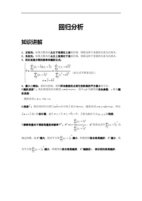
回归分析知识讲解1.正相关:如果点散布在从左下角到右上角的区域,则称这两个变量的关系为正相关。
2.负相关:如果点散布在从左上角到右下角的区域,则称这两个变量的关系为负相关。
3.回归直线方程的斜率和截距公式:⎪⎪⎩⎪⎪⎨⎧-=--=---=∑∑∑∑====xb y a xn x yx n yx x x y y x xb ni i ni ii ni i i ni i1221121)()()((此公式不要求记忆)。
4.最小二乘法:求回归直线,使得样本数据的点到它的距离的平方最小的方法。
5.随机误差e :我们把线性回归模型e a bx y ++=,其中b a ,为模型的未知参数,e 称为随机误差。
随机误差a bx y e i i i --=6.残差eˆ:我们用回归方程a x b y ˆˆˆ+=中的y ˆ估计a bx +,随机误差)(a bx y e +-=,所以y y e ˆˆ-=是e 的估计量,故a x b y y y e ii i i i ˆˆˆˆ--=-=,e ˆ称为相应于点),(i i y x 的残差。
7.解释变量对于预报变量的贡献率2R :∑∑==---=ni ini iy yyy R 12122)()ˆ(1,2R 的表达式中21)(∑=-ni i y y 为确定的数,故2R 越大,残差平方和21)ˆ(∑=-ni i yy 越小,即模型的拟合效果越好;2R 越小,残差平方和21)ˆ(∑=-ni i yy 越大,即模型的拟合效果越差。
2R 越接近1,表示回归效果越好。
典例精讲一.选择题(共12小题)1.(2018春•禅城区校级期末)在线性回归模型中,分别选择了4个不同的模型,它们的相关指数R2依次为0.36、0.95、0.74、0.81,其中回归效果最好的模型的相关指数R2为()A.0.95B.0.81C.0.74D.0.362.(2017秋•黄陵县校级月考)一项研究要确定是否能够根据施肥量预测作物的产量.这里的被解释变量是()A.作物的产量B.施肥量C.试验者D.降雨量或其他解释产量的变量3.(2017秋•荆州区校级月考)已知变量x和y的统计数据如表x681012y2356根据上表可得回归直线方程y^=0.7x+a,据此可以预测,当x=14时,y=()A.7.2B.7.5C.7.8D.8.14.(2017春•临夏市校级月考)设有一个回归方程y∧=﹣6.5x+6,变量x每增加一个单位时,变量y∧平均()A.增加6.5个单位B.增加6个单位C.减少6.5个单位D.减少6个单位5.(2017春•伊春区校级期末)某商店统计了最近6个月某商品的进份x与售价y(单位:元)的对应数据如表:x3528912y46391214假设得到的关于x和y之间的回归直线方程是y∧=bx+a,那么该直线必过的定点是()A.(8,6)B.(5,7)C.(8,6.5)D.(6.5,8)6.(2017春•商丘期末)对两个变量x和y进行回归分析,得到一组样本数据:(x1,y1),(x2,y2),…(x n,y n),则下列说法中不正确的是()A.由样本数据得到的回归方程∧y=b∧x+a∧必过样本中心(x−,y−)B.残差平方和越小的模型,拟合的效果越好C.若变量y和x之间的相关系数为r=﹣0.9362,则变量和之间具有线性相关关系D.用相关指数R2来刻画回归效果,R2越小,说明模型的拟合效果越好7.(2017春•三元区校级期中)a,b,c,d四个人各自对两个变量x,y进行相关性的测试试验,并用回归分析方法分别求得相关指数R2与残差平方和m(如表),则这四位同学中,()同学的试验结果体现两个变量x,y有更强的相关性.a b c dr0.800.760.670.82m10011312199 A.a B.b C.c D.d8.(2017春•中原区校级期中)下列可以用来分析身高和体重之间的关系的是( ) A .残差分析 B .回归分析 C .等高条形图 D .独立性检验9.(2017春•乾安县校级月考)对两个变量进行回归分析,则下列说法中不正确的是( )A .有样本数据得到的回归方程y ∧=b ∧x +a ∧必经过样本中心(x ,y ) B .残差平方和越大,模型的拟合效果越好C .用R 2来刻画回归效果,R 2越大,说明模型的拟合效果越好D .若散点图中的样本呈条状分布,则变量y 和x 之间具有线性相关关系10.(2017春•赣州期中)两个变量y 与x 的回归模型中,分别选择了4个不同模型,它们对应的回归系数r 如下,其中变量之间线性相关程度最高的模型是( )A .模型1对应的r 为﹣0.98B .模型2对应的r 为0.80C .模型3对应的r 为0.50D .模型4对应的r 为﹣0.2511.(2016秋•武昌区校级期末)对于给定的样本点所建立的模型A 和模型B ,它们的残差平方和分别是a 1,a 2,R 2的值分别为b 1,b 2,下列说法正确的是( )A .若a 1<a 2,则b 1<b 2,A 的拟合效果更好B .若a 1<a 2,则b 1<b 2,B 的拟合效果更好C .若a 1<a 2,则b 1>b 2,A 的拟合效果更好D .若a 1<a 2,则b 1>b 2,B 的拟合效果更好12.(2017•泸州模拟)某研究机构对儿童记忆能力x和识图能力y进行统计分析,得到如下数据:记忆能力x46810识图能力y3568由表中数据,求得线性回归方程为y^=45x+a^,若某儿童的记忆能力为12时,则他的识图能力为()A.9.2B.9.5C.9.8D.10二.填空题(共5小题)13.(2009春•通州区期末)某兴趣小组随机抽取了50个家庭的年可支收入x(单位:元)与年家庭消费y(单位:元)的数据,发现x和y之间具有较强的线性相关关系,回归系数约为0.5,回归街区约为380,据此可以估计某家庭年可支配收入15000元,改家庭年消费大约元.14.若施化肥量x与小麦产量y之间的回归方程为y^=250+4x(单位:kg),当施化肥量为50kg时,预计小麦产量为kg.15.(2017秋•扶余县校级期末)对于回归直线方程y^=4.75x+257,当x=28时,y 的估计值为.16.(2017春•青山区校级期末)两个相关变量的关系如下表x1236y 2 7﹣n 12 19+n利用最小二乘法得到线性回归方程为y =bx +a ,已知a ﹣b=2,则3a +b= .17.(2016秋•新余期末)一组数据中,经计算x =10,y =4,回归直线的斜率为0.6,则利用回归直线方程估计当x=12时,y= .三.解答题(共3小题)18.(2013春•蓟县期中)某种产品的广告费用支出x (万元)与销售额y (万元)之间有如下的对应数据: x 2 4 5 6 8 y3040605070(1)画出散点图; (2)求回归直线方程;(3)据此估计广告费用为9万元时,销售收入y 的值.参考公式:回归直线的方程y =bx +a ,其中b=∑n i=1(x 1−x)(y i −y)=∑ni=1x i y i −nxy∑i=1x i 2−nx2,a=y ﹣b x .19.我国1993年至2002年的国内生产总值(GDP )的数据如下:年份 GDP/亿元 1993 34634.4 1994 46759.4 1995 58478.1 199667884.61997 74462.6 1998 78345.2 1999 82067.5 2000 89468.1 2001 97314.8 2002104790.6(1)作GDP 和年份的散点图,根据该图猜想它们之间的关系是什么. (2)建立年份为解释变量,GDP 为预报变量的回归模型,并计算残差. (3)根据你得到的模型,预报2003年的GDP ,看看你的预报与实际GDP (117251.9亿元).(4)你认为这个模型能较好的刻画GDP 和年份关系吗?请说明理由.20.改革开放以来,我国高等教育事业有了突飞猛进的发展,有人记录了某村2001到2005年五年间每年考入大学的人数,为了方便计算,2001年编号为1,2002年编号为2,…,2005年编号为5,数据如下: 年份(x ) 1 2 3 4 5 人数(y )3581113求y 关于x 的回归方程y ^=b ^x +a ^所表示的直线必经的点.。

回归分析讲义范文回归分析是一种统计方法,用于研究两个或更多变量之间的关系。
它是一种预测性建模方法,可以用来预测因变量的值,基于独立变量的值。
回归分析广泛应用于经济学、金融学、社会科学和自然科学等领域。
回归分析的基本思想是建立一个数学模型,通过寻找最佳拟合线来描述自变量和因变量之间的关系。
最常用的回归模型是线性回归模型,其中自变量和因变量之间的关系可以用一条直线表示。
但是,回归分析也可以应用于非线性关系,如二次、指数和对数关系等。
线性回归模型的一般形式是:Y=β0+β1X1+β2X2+...+βnXn+ε其中Y是因变量,X1,X2,...,Xn是自变量,β0,β1,...,βn是模型的参数,ε是误差项。
回归分析的目标是估计模型的参数,以最小化观测值与拟合值之间的残差平方和。
通常使用最小二乘法来估计参数。
最小二乘法通过最小化残差平方和来确定最佳拟合线。
除了估计模型的参数,回归分析还提供了一些统计指标来评估模型的拟合程度和预测能力。
其中最常见的指标是决定系数(R-squared),它表示模型解释了因变量的变异性的比例。
R-squared的取值范围是0到1,值越接近1表示模型拟合得越好。
此外,回归分析还可以用来评估自变量的影响大小和统计显著性。
通过估计参数的标准误差和计算置信区间,可以确定自变量的影响是否显著。
回归分析的前提是自变量和因变量之间存在关系。
如果变量之间没有明显的关系,回归模型将不具备解释能力。
此外,回归分析还要求数据满足一些假设,如线性关系、多元正态分布和同方差性。
回归分析有许多扩展和改进的方法。
常见的包括多元回归分析、逐步回归、岭回归和逻辑回归等。
多元回归分析用于研究多个自变量对因变量的影响,逐步回归用于选择最佳自变量子集,岭回归用于解决多重共线性问题,逻辑回归用于二元因变量或多元因变量。
总之,回归分析是一种重要的统计方法,可以用于研究变量之间的关系和预测因变量的值。
通过建立数学模型、估计参数和评估拟合程度,回归分析可以为决策提供有用的信息和洞察力。
Class 5: ANOVA (Analysis of Variance) andF-testsI.What is ANOVAWhat is ANOVA? ANOVA is the short name for the Analysis of Variance. The essence ofANOVA is to decompose the total variance of the dependent variable into two additivecomponents, one for the structural part, and the other for the stochastic part, of a regression. Today we are going to examine the easiest case.II.ANOVA: An Introduction Let the model beεβ+= X y .Assuming x i is a column vector (of length p) of independent variable values for the i th'observation,i i i εβ+='x y .Then is the predicted value. sum of squares total:[]∑-=2Y y SST i[]∑-+-=2'x b 'x y Y b i i i[][][][]∑∑∑-+-+-=Y -b 'x b 'x y 2Y b 'x b 'x y 22i i i i i i[][]∑∑-+=22Y b 'x e i ibecause .This is always true by OLS. = SSE + SSRImportant: the total variance of the dependent variable is decomposed into two additive parts: SSE, which is due to errors, and SSR, which is due to regression. Geometric interpretation: [blackboard ]Decomposition of VarianceIf we treat X as a random variable, we can decompose total variance to the between-group portion and the within-group portion in any population:()()()i i i x y εβV 'V V +=Prove:()()i i i x y εβ+='V V()()()i i i i x x εβεβ,'Cov 2V 'V ++=()()iix εβV 'V +=(by the assumption that ()0 ,'Cov =εβk x , for all possible k.)The ANOVA table is to estimate the three quantities of equation (1) from the sample.As the sample size gets larger and larger, the ANOVA table will approach the equation closer and closer.In a sample, decomposition of estimated variance is not strictly true. We thus need toseparately decompose sums of squares and degrees of freedom. Is ANOVA a misnomer?III.ANOVA in MatrixI will try to give a simplied representation of ANOVA as follows:[]∑-=2Y y SST i ()∑-+=i i y Y 2Y y 22∑∑∑-+=i i y Y 2Y y 22∑-+=222Y n 2Y n y i (because ∑=Y n y i )∑-=22Y n y i2Y n y 'y -=y J 'y n /1y 'y -= (in your textbook, monster look)SSE = e'e[]∑-=2Y b 'x SSR i()()[]∑-+=Y b 'x 2Y b 'x 22i i()[]()∑∑-+=b 'x Y 2Y n b 'x 22i i()[]()∑∑--+=i i ie y Y 2Y n b 'x 22()[]∑-+=222Y n 2Y n b 'x i(because ∑∑==0e ,Y n y i i , as always)()[]∑-=22Yn b 'x i2Y n Xb X'b'-=y J 'y n /1y X'b'-= (in your textbook, monster look)IV.ANOVA TableLet us use a real example. Assume that we have a regression estimated to be y = - 1.70 + 0.840 xANOVA TableSOURCE SS DF MS F with Regression 6.44 1 6.44 6.44/0.19=33.89 1, 18Error 3.40 18 0.19 Total 9.8419We know , , , , . If we know that DF for SST=19, what is n?n= 205.220/50Y ==84.95.25.22084.134Y n y SST 22=⨯⨯-=-=∑i()[]∑-+=0.1250.84x 1.7-SSR 2i[]∑-⨯⨯⨯-⨯+⨯=0.125x 84.07.12x 84.084.07.17.12i i= 20⨯1.7⨯1.7+0.84⨯0.84⨯509.12-2⨯1.7⨯0.84⨯100- 125.0 = 6.44SSE = SST-SSR=9.84-6.44=3.40DF (Degrees of freedom): demonstration. Note: discounting the intercept when calculating SST. MS = SS/DFp = 0.000 [ask students].What does the p-value say?V.F-TestsF-tests are more general than t-tests, t-tests can be seen as a special case of F-tests.If you have difficulty with F-tests, please ask your GSIs to review F-tests in the lab. F-tests takes the form of a fraction of two MS's.MSR/MSE F ,=df2df1An F statistic has two degrees of freedom associated with it: the degree of freedom inthe numerator, and the degree of freedom in the denominator.An F statistic is usually larger than 1. The interpretation of an F statistics is thatwhether the explained variance by the alternative hypothesis is due to chance. In other words, the null hypothesis is that the explained variance is due to chance, or all the coefficients are zero.The larger an F-statistic, the more likely that the null hypothesis is not true. There is atable in the back of your book from which you can find exact probability values.In our example, the F is 34, which is highly significant. VI.R2R 2 = SSR / SSTThe proportion of variance explained by the model. In our example, R-sq = 65.4%VII.What happens if we increase more independent variables. 1.SST stays the same. 2.SSR always increases. 3.SSE always decreases. 4.R2 always increases. 5.MSR usually increases. 6.MSE usually decreases.7.F-test usually increases.Exceptions to 5 and 7: irrelevant variables may not explain the variance but take up degrees of freedom. We really need to look at the results.VIII.Important: General Ways of Hypothesis Testing with F-Statistics.All tests in linear regression can be performed with F-test statistics. The trick is to run"nested models."Two models are nested if the independent variables in one model are a subset or linearcombinations of a subset (子集)of the independent variables in the other model.That is to say. If model A has independent variables (1, , ), and model B has independent variables (1, , , ), A and B are nested. A is called the restricted model; B is called less restricted or unrestricted model. We call A restricted because A implies that . This is a restriction.Another example: C has independent variable (1, , + ), D has (1, + ). C and A are not nested.C and B are nested.One restriction in C: . C andD are nested.One restriction in D: . D and A are not nested.D and B are nested: two restriction in D: 32ββ=; 0=1β.We can always test hypotheses implied in the restricted models. Steps: run tworegression for each hypothesis, one for the restricted model and one for the unrestricted model. The SST should be the same across the two models. What is different is SSE and SSR. That is, what is different is R2. Let()()df df SSE ,df df SSE u u r r ==;df df ()()0u r u r r u n p n p p p -=---=-<Use the following formulas:()()()()(),SSE SSE /df SSE df SSE F SSE /df r u r u dfr dfu dfu u u---=or()()()()(),SSR SSR /df SSR df SSR F SSE /df u r u r dfr dfu dfu u u---=(proof: use SST = SSE+SSR)Note, df(SSE r )-df(SSE u ) = df(SSR u )-df(SSR r ) =df ∆,is the number of constraints (not number of parameters) implied by the restricted modelor()()()22,2R R /df F 1R /dfur dfr dfu dfuuu--∆=- Note thatdf 1df ,2F t =That is, for 1df tests, you can either do an F-test or a t-test. They yield the same result. Another way to look at it is that the t-test is a special case of the F test, with the numerator DF being 1.IX.Assumptions of F-testsWhat assumptions do we need to make an ANOVA table work?Not much an assumption. All we need is the assumption that (X'X) is not singular, so that the least square estimate b exists.The assumption of =0 is needed if you want the ANOVA table to be an unbiased estimate of the true ANOVA (equation 1) in the population. Reason: we want b to be an unbiased estimator of , and the covariance between b and to disappear.For reasons I discussed earlier, the assumptions of homoscedasticity and non-serial correlation are necessary for the estimation of .The normality assumption that (i is distributed in a normal distribution is needed for small samples.X.The Concept of IncrementEvery time you put one more independent variable into your model, you get an increase in . We sometime called the increase "incremental ." What is means is that more variance is explained, or SSR is increased, SSE is reduced. What you should understand is that the incremental attributed to a variable is always smaller than the when other variables are absent.XI.Consequences of Omitting Relevant Independent VariablesSay the true model is the following:0112233i i i i i y x x x ββββε=++++.But for some reason we only collect or consider data on . Therefore, we omit in the regression. That is, we omit in our model. We briefly discussed this problem before. The short story is that we are likely to have a bias due to the omission of a relevant variable in the model. This is so even though our primary interest is to estimate the effect of or on y. Why? We will have a formal presentation of this problem.XII.Measures of Goodness-of-FitThere are different ways to assess the goodness-of-fit of a model.A. R2R2 is a heuristic measure for the overall goodness-of-fit. It does not have an associated test statistic.R 2 measures the proportion of the variance in the dependent variable that is “explained” by the model: R 2 =SSESSR SSRSST SSR +=B.Model F-testThe model F-test tests the joint hypotheses that all the model coefficients except for the constant term are zero.Degrees of freedoms associated with the model F-test: Numerator: p-1Denominator: n-p.C.t-tests for individual parametersA t-test for an individual parameter tests the hypothesis that a particular coefficient is equal to a particular number (commonly zero).tk = (bk- (k0)/SEk, where SEkis the (k, k) element of MSE(X ’X)-1, with degree of freedom=n-p. D.Incremental R2Relative to a restricted model, the gain in R 2 for the unrestricted model: ∆R 2= R u 2- R r 2E.F-tests for Nested ModelIt is the most general form of F-tests and t-tests.()()()()(),SSE SSE /df SSE df SSE F SSE /df r u r dfu dfr u dfu u u---=It is equal to a t-test if the unrestricted and restricted models differ only by one single parameter.It is equal to the model F-test if we set the restricted model to the constant-only model.[Ask students] What are SST, SSE, and SSR, and their associated degrees of freedom, for the constant-only model?Numerical ExampleA sociological study is interested in understanding the social determinants of mathematical achievement among high school students. You are now asked to answer a series of questions. The data are real but have been tailored for educational purposes. The total number of observations is 400. The variables are defined as: y: math scorex1: father's education x2: mother's educationx3: family's socioeconomic status x4: number of siblings x5: class rankx6: parents' total education (note: x6 = x1 + x2) For the following regression models, we know: Table 1 SST SSR SSE DF R 2 (1) y on (1 x1 x2 x3 x4) 34863 4201 (2) y on (1 x6 x3 x4) 34863 396 .1065 (3) y on (1 x6 x3 x4 x5) 34863 10426 24437 395 .2991 (4) x5 on (1 x6 x3 x4) 269753 396 .02101.Please fill the missing cells in Table 1.2.Test the hypothesis that the effects of father's education (x1) and mother's education (x2) on math score are the same after controlling for x3 and x4.3.Test the hypothesis that x6, x3 and x4 in Model (2) all have a zero effect on y.4.Can we add x6 to Model (1)? Briefly explain your answer.5.Test the hypothesis that the effect of class rank (x5) on math score is zero after controlling for x6, x3, and x4.Answer: 1. SST SSR SSE DF R 2 (1) y on (1 x1 x2 x3 x4) 34863 4201 30662 395 .1205 (2) y on (1 x6 x3 x4) 34863 3713 31150 396 .1065 (3) y on (1 x6 x3 x4 x5) 34863 10426 24437 395 .2991 (4) x5 on (1 x6 x3 x4) 275539 5786 269753 396 .0210Note that the SST for Model (4) is different from those for Models (1) through (3). 2.Restricted model is 01123344()y b b x x b x b x e =+++++Unrestricted model is ''''''011223344y b b x b x b x b x e =+++++(31150 - 30662)/1F 1,395 = -------------------- = 488/77.63 = 6.29 30662 / 395 3.3713 / 3F 3,396 = --------------- = 1237.67 / 78.66 = 15.73 31150 / 3964.No. x6 is a linear combination of x1 and x2. X'X is singular.5.(31150 - 24437)/1F 1,395 = -------------------- = 6713 / 61.87 = 108.50 24437/395t = 10.42t ===。