数字图像处理教程(matlab版)

实验报告实验一图像的傅里叶变换（旋转性质）实验二图像的代数运算实验三filter2实现均值滤波实验四图像的缩放朱锦璐04085122实验一图像的傅里叶变换（旋转性质）一、实验内容对图（1.1）的图像做旋转，观察原图的傅里叶频谱和旋转后的傅里叶频谱的对应关系。

图（1.1）二、实验原理首先借助极坐标变换x=rcosθ,y=rsinθ,u=wcosϕ,v=wsinϕ,,将f(x,y)和F(u,v)转换为f(r,θ)和F（w，ϕ）.f(x,y) <=> F(u，v)f(rcosθ,rsinθ)<=> F(wcosϕ，wsinϕ)经过变换得f( r,θ+θ。

)<=>F(w,ϕ+θ。

)上式表明，对f(x,y)旋转一个角度θ。

对应于将其傅里叶变换F(u，v)也旋转相同的角度θ。

F(u,v)到f(x,y)也是一样。

三、实验方法及程序选取一幅图像，进行离散傅里叶变换，在对其进行一定角度的旋转，进行离散傅里叶变换。

>> I=zeros(256,256); %构造原始图像I(88:168,120:136)=1; %图像范围256*256，前一值是纵向比，后一值是横向比figure(1);imshow(I); %求原始图像的傅里叶频谱J=fft2(I);F=abs(J);J1=fftshift(F);figure(2)imshow(J1,[5 50])J=imrotate(I,45,'bilinear','crop'); %将图像逆时针旋转45°figure(3);imshow(J) %求旋转后的图像的傅里叶频谱J1=fft2(J);F=abs(J1);J2=fftshift(F);figure(4)imshow(J2,[5 50])四、实验结果与分析实验结果如下图所示（1.2）原图像（1.3）傅里叶频谱（1.4）旋转45°后的图像（1.5）旋转后的傅里叶频谱以下为放大的图（1.6）原图像（1.7）傅里叶频谱（1.8）旋转45°后的图像（1.9）旋转后的傅里叶频谱由实验结果可知1、从旋转性质来考虑，图（1.8）是图（1.6）逆时针旋转45°后的图像，对比图（1.7）和图（1.9）可知，频域图像也逆时针旋转了45°2、从尺寸变换性质来考虑，如图（1.6）和图（1.7）、图（1.8）和图（1.9）可知，原图像和其傅里叶变换后的图像角度相差90°，由此可知，时域中的信号被压缩，到频域中的信号就被拉伸。

第一章1. 什么是图像？如何区分数字图像和模拟图像？模拟图像和数字图像如何相互转换？答：图像是当光辐射能量照在物体上，经过反射或透射，或由发光物体本身发出的光能量，在人的视觉器官中所重现出的物体的视觉信息。

数字图像将图像看成是许多大小相同、形状一致的像素组成。

这样，数字图像可以用二维矩阵表示。

将自然界的图像通过光学系统成像并由电子器件或系统转化为模拟图像（连续图像）信号，再由模拟/数字转化器（ADC）得到原始的数字图像信号。

图像的数字化包括离散和量化两个主要步骤。

在空间将连续坐标过程称为离散化，而进一步将图像的幅度值（可能是灰度或色彩）整数化的过程称为量化。

2. 什么是数字图像处理？答：数字图像处理(Digital Image Processing)是通过计算机对图像进行去除噪声、增强、复原、分割、提取特征等处理的方法和技术。

3. 数字图像处理系统有哪几部分组成？各部分的主要功能和常见设备有哪些？答：一个基本的数字图像处理系统由图像输入、图像存储、图像输出、图像通信、图像处理和分析5个模块组成，如下图所示。

各个模块的作用分别为：图像输入模块：图像输入也称图像采集或图像数字化，它是利用图像采集设备（如数码照相机、数码摄像机等）来获取数字图像，或通过数字化设备（如图像扫描仪）将要处理的连续图像转换成适于计算机处理的数字图像。

图像存储模块：主要用来存储图像信息。

图像输出模块：将处理前后的图像显示出来或将处理结果永久保存。

图像通信模块：对图像信息进行传输或通信。

图像处理与分析模块：数字图像处理与分析模块包括处理算法、实现软件和数字计算机，以完成图像信息处理的所有功能。

4. 试述人眼的主要特性。

答：（1）、人眼的视觉机理。

视网膜上有大量的杆状细胞和锥状细胞，锥状细胞能辨别光的颜色，而杆状细胞感光灵敏度高，但不能辨色。

（2）、人眼的视敏特性。

指人眼对不同波长的光具有不同的敏感程度。

（3）、人眼的亮度感觉。

亮度感觉范围指人眼所能感觉到的最大亮度与最小亮度之间的范围。

% *-*--*-*-*-*-*-*-*-*-*-*-*图像处理*-*-*-*-*-*-*-*-*-*-*-*%{% （一）图像文件的读/写A=imread('drum.jpg'); % 读入图像imshow(A); % 显示图像imwrite(A,'drum.jpg');info=imfinfo('drum.jpg') % 查询图像文件信息% 用colorbar函数将颜色条添加到坐标轴对象中RGB=imread('drum.jpg');I=rgb2gray(RGB); % 把RGB图像转换成灰度图像h=[1 2 1;0 0 0;-1 -2 -1];I2=filter2(h,I);imshow(I2,[]);colorbar('vert') % 将颜色条添加到坐标轴对象中% wrap函数将图像作为纹理进行映射A=imread('4.jpg');imshow(A);I=rgb2gray(RGB);[x,y,z]=sphere;warp(x,y,z,I); % 用warp函数将图像作为纹理进行映射%}% subimage函数实现一个图形窗口中显示多幅图像RGB=imread('drum.jpg');I=rgb2gray(RGB);subplot(1,2,1);subimage(RGB); % subimage函数实现一个图形窗口中显示多幅图像subplot(1,2,2),subimage(I);% *-*--*-*-*-*-*-*-*-*-*-*-*图像处理*-*-*-*-*-*-*-*-*-*-*-*% （二）图像处理的基本操作% ----------------图像代数运算------------------%{% imadd函数实现两幅图像的相加或给一幅图像加上一个常数% 给图像每个像素都增加亮度I=imread('4.jpg');J=imadd(I,100); % 给图像增加亮度subplot(1,2,1),imshow(I);title('原图');subplot(1,2,2),imshow(J);title('增加亮度图');%% imsubtract函数实现将一幅图像从另一个图像中减去或减去一个常数I=imread('drum.jpg');J=imsubtract(I,100); % 给图像减去亮度subplot(1,2,1),imshow(I);%% immultiply实现两幅图像的相乘或者一幅图像的亮度缩放I=imread('drum.jpg');J=immultiply(I,2); % 进行亮度缩放subplot(1,2,1),imshow(I);subplot(1,2,2),imshow(J);%% imdivide函数实现两幅图像的除法或一幅图像的亮度缩放I=imread('4.jpg');J=imdivide(I,0.5); % 图像的亮度缩放subplot(1,2,1),imshow(I);subplot(1,2,2),imshow(J);%}% ----------------图像的空间域操作------------------%{% imresize函数实现图像的缩放J=imread('4.jpg');subplot(1,2,1),imshow(J);title('原图');X1=imresize(J,0.2); % 对图像进行缩放subplot(1,2,2),imshow(X1);title('缩放图');%% imrotate函数实现图像的旋转I=imread('drum.jpg');J=imrotate(I,50,'bilinear'); % 对图像进行旋转subplot(1,2,1),imshow(I);subplot(1,2,2),imshow(J);%% imcrop函数实现图像的剪切I=imread('drum.jpg');I2=imcrop(I,[1 100 130 112]); % 对图像进行剪切subplot(1,2,1),imshow(I);subplot(1,2,2),imshow(I2);%}% ----------------特定区域处理------------------%{% roipoly函数用于选择图像中的多边形区域I=imread('4.jpg');c=[200 250 278 248 199 172];r=[21 21 75 121 121 75];BW=roipoly(I,c,r); % roipoly函数选择图像中的多边形区域subplot(1,2,1),imshow(I);subplot(1,2,2),imshow(BW);%% roicolor函数式对RGB图像和灰度图像实现按灰度或亮度值选择区域进行处理a=imread('4.jpg');subplot(2,2,1),imshow(a);I=rgb2gray(a);BW=roicolor(I,128,225); % 按灰度值选择的区域subplot(2,2,4),imshow(BW);%% ploy2mask 函数转化指定的多边形区域为二值掩模x=[63 186 54 190 63];y=[60 60 209 204 601];bw=poly2mask(x,y,256,256); % 转化指定的多边形区域为二值掩模imshow(bw);hold onplot(x,y,'r','LineWidth',2);hold off%% roifilt2函数实现区域滤波a=imread('4.jpg');I=rgb2gray(a);c=[200 250 278 248 199 172];r=[21 21 75 121 121 75];BW=roipoly(I,c,r); % roipoly函数选择图像中的多边形区域h=fspecial('unsharp');J=roifilt2(h,I,BW); % 区域滤波subplot(1,2,1),imshow(I);subplot(1,2,2),imshow(J);%% roifill函数实现对特定区域进行填充a=imread('4.jpg');I=rgb2gray(a);c=[200 250 278 248 199 172];r=[21 21 75 121 121 75];J=roifill(I,c,r); % 对特定区域进行填充subplot(1,2,1),imshow(I);subplot(1,2,2),imshow(J);%}% ----------------图像变换------------------%{% fft2 和ifft2函数分别是计算二维的快速傅里叶变换和反变换f=zeros(100,100);subplot(1,2,1);imshow(f);f(20:70,40:60)=1;subplot(1,2,2);imshow(f);F=fft2(f); % 计算二维的快速傅里叶变换F2=log(abs(F));% 对幅值对对数figure;subplot(1,2,1),imshow(F),colorbar;subplot(1,2,2),imshow(F2),colorbar;%% fftsshift 函数实现了补零操作和改变图像显示象限f=zeros(100,100);subplot(2,2,1),imshow(f);title('f')f(10:70,40:60)=1;subplot(2,2,2),imshow(f);title('f取后')F=fft2(f,256,256);subplot(2,2,3),imshow(F);title('F')F2=fftshift(F); % 实现补零操作subplot(2,2,4),imshow(F2);title('F2')figure,imshow(log(abs(F2)));title('log(|F2|)')%% dct2 函数采用基于快速傅里叶变换的算法，用于实现较大输入矩阵的离散余弦变换% idct2 函数实现图像的二维逆离散余弦变换RGB=imread('drum.jpg');I=rgb2gray(RGB);J=dct2(I); % 对I进行离散余弦变换imshow(log(abs(J))),title('对原图离散后取对数'),colorbar;J(abs(J)<10)=0;K=idct2(J); % 图像的二维逆离散余弦变换figure,imshow(I),title('原灰度图')figure,imshow(K,[0,255]);title('逆离散变换');%% dctmtx 函数用于实现较小输入矩阵的离散余弦变figure;RGB=imread('4.jpg');I=rgb2gray(RGB);subplot(3,2,1),imshow(I),title('原灰度图');I=im2double(I);subplot(3,2,2),imshow(I),title('取双精度后');T=dctmtx(8); % 离散余弦变换subplot(3,2,3),imshow(I),title('离散余弦变换后');B=blkproc(I,[8,8],'P1*x*P2',T,T');subplot(3,2,4),imshow(B),title('blkproc作用I后的B');mask=[ 1 1 1 1 0 0 0 01 1 1 0 0 0 0 01 1 0 0 0 0 0 01 0 0 0 0 0 0 00 0 0 0 0 0 0 00 0 0 0 0 0 0 00 0 0 0 0 0 0 00 0 0 0 0 0 0 0 ];B2=blkproc(B,[8,8],'P1.*x',mask);subplot(3,2,5),imshow(B2),title('blkproc作用B后的B2');I2=blkproc(B2,[8,8],'P1*x*P2',T',T);subplot(3,2,6),imshow(I2),title('blkproc作用B2后的I2');%% edge函数用于提取图像的边缘RGB=imread('4.jpg');I=rgb2gray(RGB);BW=edge(I);imshow(I);figure,imshow(BW);%% radon 函数用来计算指定方向上图像矩阵的投影RGB=imread('4.jpg');I=rgb2gray(RGB);BW=edge(I);theta=0:179;[R,XP]=radon(BW,theta); % 图像矩阵的投影figure,imagesc(theta,XP,R);colormap(hot);xlabel('\theta(degrees)');ylabel('x\prime');title('R_{\theta}(x\prime)');colorbar;%}% ----------------图像增强、分割和编码------------------%{% imhist 函数产生图像的直方图A=imread('4.jpg');B=rgb2gray(A);subplot(2,1,1),imshow(B);subplot(2,1,2),imhist(B);%% histeq 函数用于对图像的直方图均衡化A=imread('4.jpg');B=rgb2gray(A);subplot(2,1,1),imshow(B);subplot(2,1,2),imhist(B);C=histeq(B); % 对图像B进行均衡化figure;subplot(2,1,1),imshow(C);subplot(2,1,2),imhist(C);%% filter2 函数实现均值滤波a=imread('4.jpg');I=rgb2gray(a);subplot(2,2,1),imshow(I);K1=filter2(fspecial('average',3),I)/255; % 3*3的均值滤波K2=filter2(fspecial('average',5),I)/255; % 5*5的均值滤波K3=filter2(fspecial('average',7),I)/255; % 7*7的均值滤波subplot(2,2,2),imshow(K1);subplot(2,2,3),imshow(K2);subplot(2,2,4),imshow(K3);%% wiener2 函数实现Wiener（维纳）滤波a=imread('4.jpg');I=rgb2gray(a);subplot(2,2,1),imshow(I);K1=wiener2(I,[3,3]); % 3*3 wiener滤波K2=wiener2(I,[5,5]); % 5*5 wiener滤波K3=wiener2(I,[7,7]); % 7*7 wiener滤波subplot(2,2,2),imshow(K1);subplot(2,2,3),imshow(K2);subplot(2,2,4),imshow(K3);%% medfilt2 函数实现中值滤波a=imread('4.jpg');I=rgb2gray(a);subplot(2,2,1),imshow(I);K1=medfilt2(I,[3,3]); % 3*3 中值滤波K2=medfilt2(I,[5,5]); % 5*5 中值滤波K3=medfilt2(I,[7,7]); % 7*7 中值滤波subplot(2,2,2),imshow(K1);subplot(2,2,3),imshow(K2);subplot(2,2,4),imshow(K3);%}% ----------------图像模糊及复原------------------%{% deconvwnr 函数：使用维纳滤波器I=imread('qier.jpg');imshow(I);% 对图像进行模糊处理LEN=31;THETA=11;PSF1=fspecial('motion',LEN,THETA); % 运动模糊PSF2=fspecial('gaussian',10,5); % 高斯模糊Blurred1=imfilter(I,PSF1,'circular','conv'); % 得到运动模糊图像Blurred2=imfilter(I,PSF2,'conv'); % 得到高斯噪声模糊图像figure;subplot(1,2,1);imshow(Blurred1);title('Blurred1--"motion"'); subplot(1,2,2);imshow(Blurred2);title('Blurred2--"gaussian"');% 对模糊图像加噪声V=0.002;BlurredNoisy1=imnoise(Blurred1,'gaussian',0,V); % 加高斯噪声BlurredNoisy2=imnoise(Blurred2,'gaussian',0,V); % 加高斯噪声figure;subplot(1,2,1);imshow(BlurredNoisy1);title('BlurredNoisy1'); subplot(1,2,2);imshow(BlurredNoisy2);title('BlurredNoisy2');% 进行维纳滤波wnr1=deconvwnr(Blurred1,PSF1); % 维纳滤波wnr2=deconvwnr(Blurred2,PSF2); % 维纳滤波figure;subplot(1,2,1);imshow(wnr1);title('Restored1,True PSF'); subplot(1,2,2);imshow(wnr2);title('Restored2,True PSF');%% deconvreg函数：使用约束最小二乘滤波器I=imread('qier.jpg');imshow(I);% 对图像进行模糊处理LEN=31;THETA=11;PSF1=fspecial('motion',LEN,THETA); % 运动模糊PSF2=fspecial('gaussian',10,5); % 高斯模糊Blurred1=imfilter(I,PSF1,'circular','conv'); % 得到运动模糊图像Blurred2=imfilter(I,PSF2,'conv'); % 得到高斯噪声模糊图像figure;subplot(1,2,1);imshow(Blurred1);title('Blurred1--"motion"');subplot(1,2,2);imshow(Blurred2);title('Blurred2--"gaussian"');% 对模糊图像加噪声V=0.002;BlurredNoisy1=imnoise(Blurred1,'gaussian',0,V); % 加高斯噪声BlurredNoisy2=imnoise(Blurred2,'gaussian',0,V); % 加高斯噪声figure;subplot(1,2,1);imshow(BlurredNoisy1);title('BlurredNoisy1');subplot(1,2,2);imshow(BlurredNoisy2);title('BlurredNoisy2');NP=V*prod(size(I));reg1=deconvreg(BlurredNoisy1,PSF1,NP); % 约束最小二乘滤波reg2=deconvreg(BlurredNoisy2,PSF2,NP); % 约束最小二乘滤波figure;subplot(1,2,1);imshow(reg1);title('Restored1 with NP');subplot(1,2,2);imshow(reg2);title('Restored2 with NP');%% deconvlucy函数：使用Lucy-Richardson滤波器I=imread('qier.jpg');imshow(I);% 对图像进行模糊处理LEN=31;THETA=11;PSF1=fspecial('motion',LEN,THETA); % 运动模糊PSF2=fspecial('gaussian',10,5); % 高斯模糊Blurred1=imfilter(I,PSF1,'circular','conv'); % 得到运动模糊图像Blurred2=imfilter(I,PSF2,'conv'); % 得到高斯噪声模糊图像figure;subplot(1,2,1);imshow(Blurred1);title('Blurred1--"motion"');subplot(1,2,2);imshow(Blurred2);title('Blurred2--"gaussian"');% 对模糊图像加噪声V=0.002;BlurredNoisy1=imnoise(Blurred1,'gaussian',0,V); % 加高斯噪声BlurredNoisy2=imnoise(Blurred2,'gaussian',0,V); % 加高斯噪声figure;subplot(1,2,1);imshow(BlurredNoisy1);title('BlurredNoisy1');subplot(1,2,2);imshow(BlurredNoisy2);title('BlurredNoisy2');luc1=deconvlucy(BlurredNoisy1,PSF1,5); % 使用Lucy-Richardson滤波luc2=deconvlucy(BlurredNoisy1,PSF1,15); % 使用Lucy-Richardson滤波figure;subplot(1,2,1);imshow(luc1);title('Restored Image,NUMIT=5'); subplot(1,2,2);imshow(luc2);title('Restored Image,NUMIT=15');%}% deconvblind 函数：使用盲卷积算法a=imread('4.jpg');I=rgb2gray(a);figure;imshow(I);title('Original Image');PSF=fspecial('motion',13,45); % 运动模糊figure;imshow(PSF);Blurred=imfilter(I,PSF,'circ','conv'); % 得到运动模糊图像figure;imshow(Blurred);title('Blurred Image');INITPSF=ones(size(PSF));[J,P]=deconvblind(Blurred,INITPSF,30); % 使用盲卷积figure;imshow(J);figure;imshow(P,[],'notruesize');% *-*--*-*-*-*-*-*-*-*-*-*-*图像处理*-*-*-*-*-*-*-*-*-*-*-* %{% 对图像进行减采样a=imread('lena.jpg');%subplot(1,4,1);figure;imshow(a);title('原图');b=rgb2gray(a);%subplot(1,4,2);figure;imshow(b);title('原图的灰度图');[wid,hei]=size(b);%---4倍减采样----quartimg=zeros(wid/2+1,hei/2+1);i1=1;j1=1;for i=1:2:widfor j=1:2:heiquartimg(i1,j1)=b(i,j);j1=j1+1;endi1=i1+1;j1=1;end%subplot(1,4,3);figure;imshow(uint8(quartimg));title('4倍减采样')% ---16倍减采样---quanrtimg=zeros(wid/4+1,hei/4+1);i1=1;j1=1;for i=1:4:widfor j=1:4:heiquanrtimg(i1,j1)=b(i,j);j1=j1+1;endi1=i1+1;j1=1;end%subplot(1,4,4);.figure;imshow(uint8(quanrtimg));title('16倍减采样');%}% 图像类型% 将图像转换为256级灰度图像，64级灰度图像，32级灰度图像，8级灰度图像，2级灰度图像a=imread('4.jpg');%figure;subplot(2,3,1);imshow(a);title('原图');b=rgb2gray(a); % 这是256灰度级的图像%figure;subplot(2,3,2);imshow(b);title('原图的灰度图像');[wid,hei]=size(b);img64=zeros(wid,hei);img32=zeros(wid,hei);img8=zeros(wid,hei);img2=zeros(wid,hei);for i=1:widfor j=j:heiimg64(i,j)=floor(b(i,j)/4); % 转化为64灰度级endend%figure;subplot(2,3,3);imshow(uint8(img64),[0,63]);title('64级灰度图像');for i=1:widfor j=1:heiimg32(i,j)=floor(b(i,j)/8);% 转化为32灰度级endend%figure;subplot(2,3,4);imshow(uint8(img32),[0,31]);title('32级灰度图像');for i=1:widfor j=1:heiimg8(i,j)=floor(b(i,j)/32);% 转化为8灰度级endend%figure;subplot(2,3,5);imshow(uint8(img8),[0,7]);title('8级灰度图像');for i=1:widfor j=1:heiimg2(i,j)=floor(b(i,j)/128);% 转化为2灰度级endend%figure;subplot(2,3,6);imshow(uint8(img2),[0,1]);title('2级灰度图像');% *-*--*-*-*-*-*-*-*-*-*-*-*图像处理*-*-*-*-*-*-*-*-*-*-*-* %{% ------------------ 图像的点运算------------------I=imread('lena.jpg');figure;subplot(1,3,1);imshow(I);title('原图的灰度图');J=imadjust(I,[0.3;0.6],[0.1;0.9]); % 设置灰度变换的范围subplot(1,3,2);imshow(J);title('线性扩展');I1=double(I); % 将图像转换为double类型I2=I1/255; % 归一化此图像C=2; % 非线性扩展函数的参数K=C*log(1+I2); % 对图像的对数变换subplot(1,3,3);imshow(K);title('非线性扩展');M=255-I;figure;subplot(1,3,1);imshow(M);title('灰度倒置');N1=im2bw(I,0.4); % 将此图像二值化，阈值为0.4N2=im2bw(I,0.7); % 将此图像二值化，阈值为0.7 subplot(1,3,2);imshow(N1);title('二值化阈值0.4');subplot(1,3,3);imshow(N2);title('二值化阈值0.7');%}%{% ------------------ 图像的代数运算------------------% 将两幅图像进行加法运算I=imread('lena.jpg');I=rgb2gray(I);J=imread('rice.png');% 以下把两幅图转化为大小一样for i=1:size(I)for j=size(J):size(I)J(i,j)=0;endendI=im2double(I); % 将图像转化为double型J=im2double(J);% imshow(I);figure;imshow(J);K=I+0.3*J; % 将两幅图像相加subplot(1,3,1);imshow(I);title('人物图');subplot(1,3,2);imshow(J);title('背景图');subplot(1,3,3);imshow(K);title('相加后的图');imwrite(K,'i_lena1.jpg');%%% 将两幅图像做减运算，分离背景与原图A=imread('i_lena1.jpg');B=imread('rice.png');% 以下把两幅图转化为大小一样for i=1:size(A)for j=size(B):size(A)B(i,j)=0;endendC=A-0.3*B;a=imread('lena.jpg');subplot(2,2,1);imshow(a);title('原图图');subplot(2,2,2);imshow(A);title('混合图');subplot(2,2,3);imshow(B);title('背景图');subplot(2,2,4);imshow(C);title('分离后的图');%% 设置掩模，需要保留下来的区域，掩模图像的值为1，否则为0 A=imread('drum.jpg');A=rgb2gray(A);A=im2double(A);sizeA=size(A);subplot(1,2,1);imshow(A);title('原图');B=zeros(sizeA(1),sizeA(2)); % 设置模板B(100:400,100:500)=1;K=A.*B; % 两幅图像相乘subplot(1,2,2);imshow(K);title('局部图');%}%{% ------------------ 图像的缩放------------------A=imread('drum.jpg');B1=imresize(A,1.5); % 比例放大1.5杯，默认采用的是最近邻法进行线性插值B2=imresize(A,[420 384]); % 非比例放大到420:384C1=imresize(A,0.7); % 比例缩小0.7倍C2=imresize(A,[150 180]); % 非比例缩小到150:180figure;imshow(B1);title('比例放大图');figure;imshow(B2);title('非比例放大图');figure;imshow(C1);title('比例缩小图');figure;imshow(C2);title('非比例缩小图');% 检测非比例缩放得到的图片是否能还原到原图a=size(A)d=imresize(C2,[a(1),a(2)]);figure;imshow(d);%}% ------------------ 图像的旋转------------------I=imread('drum.jpg');J=imrotate(I,45); % 图像进行逆时针旋转，默认采用最近邻插值法进行插值处理K=imrotate(I,90); % 默认旋转出界的部分不被截出subplot(1,3,1);imshow(I);subplot(1,3,2);imshow(J);subplot(1,3,3);imshow(K);% 检测旋转后的图像是否失真P=imrotate(K,270);figure;imshow(P);。

第一部分数字图像处理实验一图像的点运算实验1.1 直方图一．实验目的1．熟悉matlab图像处理工具箱及直方图函数的使用；2．理解和掌握直方图原理和方法；二．实验设备1.PC机一台；2.软件matlab。

三．程序设计在matlab环境中，程序首先读取图像，然后调用直方图函数，设置相关参数，再输出处理后的图像。

I=imread('cameraman.tif');%读取图像subplot(1,2,1),imshow(I) %输出图像title('原始图像') %在原始图像中加标题subplot(1,2,2),imhist(I) %输出原图直方图title('原始图像直方图') %在原图直方图上加标题四．实验步骤1. 启动matlab双击桌面matlab图标启动matlab环境；2. 在matlab命令窗口中输入相应程序。

书写程序时，首先读取图像，一般调用matlab自带的图像，如:cameraman图像；再调用相应的直方图函数，设置参数；最后输出处理后的图像；3．浏览源程序并理解含义；4．运行，观察显示结果；5．结束运行，退出；五．实验结果观察图像matlab环境下的直方图分布。

(a)原始图像 (b)原始图像直方图六．实验报告要求1、给出实验原理过程及实现代码；2、输入一幅灰度图像，给出其灰度直方图结果，并进行灰度直方图分布原理分析。

实验1.2 灰度均衡一．实验目的1．熟悉matlab图像处理工具箱中灰度均衡函数的使用；2．理解和掌握灰度均衡原理和实现方法；二．实验设备1.PC机一台；2.软件matlab；三．程序设计在matlab环境中，程序首先读取图像，然后调用灰度均衡函数，设置相关参数，再输出处理后的图像。

I=imread('cameraman.tif');%读取图像subplot(2,2,1),imshow(I) %输出图像title('原始图像') %在原始图像中加标题subplot(2,2,3),imhist(I) %输出原图直方图title('原始图像直方图') %在原图直方图上加标题a=histeq(I,256); %直方图均衡化，灰度级为256subplot(2,2,2),imshow(a) %输出均衡化后图像title('均衡化后图像') %在均衡化后图像中加标题subplot(2,2,4),imhist(a) %输出均衡化后直方图title('均衡化后图像直方图') %在均衡化后直方图上加标题四．实验步骤1. 启动matlab双击桌面matlab图标启动matlab环境；2. 在matlab命令窗口中输入相应程序。

实验一MATLAB数字图像处理初步一、实验目的1、熟悉及掌握在MATLAB中能够处理哪些格式图像。

2、熟练掌握在MATLAB中读取图像，并获取图像的大小、颜色、高度、宽度等等相关信息。

3、掌握在MATLAB中按照指定要求存储一幅图像的方法。

4、熟悉数字图像矩阵的格式转换二、实验原理及知识点1、数字图像的表示和类别一幅图像可以被定义为一个二维函数f(x,y),其中x和y是空间(平面)坐标，f 在任何坐标处(x,y)处的振幅称为图像在该点的亮度。

灰度是用来表示黑白图像亮度的一个术语，而彩色图像是由单个二维图像组合形成的。

例如，在RGB彩色系统中，一幅彩色图像是由三幅独立的分量图像(红、绿、蓝)组成的。

因此，许多为黑白图像处理开发的技术适用于彩色图像处理，方法是分别处理三副独立的分量图像即可。

图像关于x和y坐标以及振幅连续。

要将这样的一幅图像转化为数字形式，就要求数字化坐标和振幅。

将坐标值数字化成为取样；将振幅数字化成为量化。

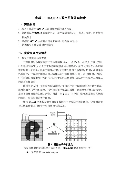
采样和量化的过程如图1所示。

因此，当f的x、y分量和振幅都是有限且离散的量时，称该图像为数字图像。

作为MATLAB基本数据类型的数值数组本身十分适于表达图像，矩阵的元素和图像的像素之间有着十分自然的对应关系。

图1 图像的采样和量化根据图像数据矩阵解释方法的不同，MATLAB把其处理为4类： 亮度图像(Intensity images)二值图像(Binary images)索引图像(Indexed images)RGB图像(RGB images)(1) 亮度图像一幅亮度图像是一个数据矩阵，其归一化的取值表示亮度。

若亮度图像的像素都是uint8类或uint16类，则它们的整数值范围分别是[0，255]和[0，65536]。

若图像是double类，则像素取值就是浮点数。

规定双精度型归一化亮度图像的取值范围是[0，1](2) 二值图像一幅二值图像是一个取值只有0和1的逻辑数组。

而一幅取值只包含0和1的uint8类数组，在MATLAB中并不认为是二值图像。

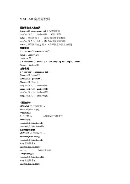
MATLAB实用源代码图像读取及灰度变换I=imread('cameraman.tif');%读取图像subplot(1,2,1),imshow(I) %输出图像title('原始图像') %在原始图像中加标题subplot(1,2,2),imhist(I) %输出原图直方图title('原始图像直方图') %在原图直方图上加标题图像旋转I = imread('cameraman.tif');figure,imshow(I);theta = 30;K = imrotate(I,theta); % Try varying the angle, theta. figure, imshow(K)边缘检测I = imread('cameraman.tif');J1=edge(I,'sobel');J2=edge(I,'prewitt');J3=edge(I,'log');subplot(1,4,1),imshow(I);subplot(1,4,2),imshow(J1);subplot(1,4,3),imshow(J2);subplot(1,4,4),imshow(J3);1.图像反转MATLAB 程序实现如下：I=imread('xian.bmp');J=double(I);J=-J+(256-1); %图像反转线性变换H=uint8(J);subplot(1,2,1),imshow(I);subplot(1,2,2),imshow(H);2.灰度线性变换MATLAB 程序实现如下：I=imread('xian.bmp');subplot(2,2,1),imshow(I);title('原始图像');axis([50,250,50,200]);axis on; %显示坐标系I1=rgb2gray(I);subplot(2,2,2),imshow(I1);title('灰度图像');axis([50,250,50,200]);axis on; %显示坐标系J=imadjust(I1,[0.1 0.5],[]); %局部拉伸，把[0.1 0.5]内的灰度拉伸为[0 1] subplot(2,2,3),imshow(J);title('线性变换图像[0.1 0.5]');axis([50,250,50,200]);grid on; %显示网格线axis on; %显示坐标系K=imadjust(I1,[0.3 0.7],[]); %局部拉伸，把[0.3 0.7]内的灰度拉伸为[0 1] subplot(2,2,4),imshow(K);title('线性变换图像[0.3 0.7]');axis([50,250,50,200]);grid on; %显示网格线axis on; %显示坐标系3.非线性变换MATLAB 程序实现如下：I=imread('xian.bmp');I1=rgb2gray(I);subplot(1,2,1),imshow(I1);title(' 灰度图像');axis([50,250,50,200]);grid on; %显示网格线axis on; %显示坐标系J=double(I1);J=40*(log(J+1));H=uint8(J);subplot(1,2,2),imshow(H);title(' 对数变换图像');axis([50,250,50,200]);grid on; %显示网格线axis on; %显示坐标系4.直方图均衡化MATLAB 程序实现如下：I=imread('xian.bmp');I=rgb2gray(I);figure;subplot(2,2,1);imshow(I);subplot(2,2,2);imhist(I);I1=histeq(I);figure;subplot(2,2,1);imshow(I1);subplot(2,2,2);imhist(I1);5. 线性平滑滤波器用MA TLAB实现领域平均法抑制噪声程序：I=imread('xian.bmp');subplot(231)imshow(I)title('原始图像')I=rgb2gray(I);I1=imnoise(I,'salt & pepper',0.02);subplot(232)imshow(I1)title(' 添加椒盐噪声的图像')k1=filter2(fspecial('average',3),I1)/255; %进行3*3模板平滑滤波k2=filter2(fspecial('average',5),I1)/255; %进行5*5模板平滑滤波k3=filter2(fspecial('average',7),I1)/255; %进行7*7模板平滑滤波k4=filter2(fspecial('average',9),I1)/255; %进行9*9模板平滑滤波subplot(233),imshow(k1);title('3*3 模板平滑滤波');subplot(234),imshow(k2);title('5*5 模板平滑滤波');subplot(235),imshow(k3);title('7*7 模板平滑滤波');subplot(236),imshow(k4);title('9*9 模板平滑滤波');6.中值滤波器用MA TLAB实现中值滤波程序如下：I=imread('xian.bmp');I=rgb2gray(I);J=imnoise(I,'salt&pepper',0.02);subplot(231),imshow(I);title('原图像');subplot(232),imshow(J);title('添加椒盐噪声图像');k1=medfilt2(J); %进行3*3模板中值滤波k2=medfilt2(J,[5,5]); %进行5*5模板中值滤波k3=medfilt2(J,[7,7]); %进行7*7模板中值滤波k4=medfilt2(J,[9,9]); %进行9*9模板中值滤波subplot(233),imshow(k1);title('3*3模板中值滤波');subplot(234),imshow(k2);title('5*5模板中值滤波');subplot(235),imshow(k3);title('7*7模板中值滤波');subplot(236),imshow(k4);title('9*9 模板中值滤波');7.用Sobel算子和拉普拉斯对图像锐化：I=imread('xian.bmp');subplot(2,2,1),imshow(I);title('原始图像');axis([50,250,50,200]);grid on; %显示网格线axis on; %显示坐标系I1=im2bw(I);subplot(2,2,2),imshow(I1);title('二值图像');axis([50,250,50,200]);grid on; %显示网格线axis on; %显示坐标系H=fspecial('sobel'); %选择sobel算子J=filter2(H,I1); %卷积运算subplot(2,2,3),imshow(J);title('sobel算子锐化图像');axis([50,250,50,200]);grid on; %显示网格线axis on; %显示坐标系h=[0 1 0,1 -4 1,0 1 0]; %拉普拉斯算子J1=conv2(I1,h,'same'); %卷积运算subplot(2,2,4),imshow(J1);title('拉普拉斯算子锐化图像');axis([50,250,50,200]);grid on; %显示网格线axis on; %显示坐标系8.梯度算子检测边缘用MA TLAB实现如下：I=imread('xian.bmp');subplot(2,3,1);imshow(I);title('原始图像');axis([50,250,50,200]);grid on; %显示网格线axis on; %显示坐标系I1=im2bw(I);subplot(2,3,2);imshow(I1);title('二值图像');axis([50,250,50,200]);grid on; %显示网格线axis on; %显示坐标系I2=edge(I1,'roberts');figure;subplot(2,3,3);imshow(I2);title('roberts算子分割结果');axis([50,250,50,200]);grid on; %显示网格线axis on; %显示坐标系I3=edge(I1,'sobel');subplot(2,3,4);imshow(I3);title('sobel算子分割结果');axis([50,250,50,200]);grid on; %显示网格线axis on; %显示坐标系I4=edge(I1,'Prewitt');subplot(2,3,5);imshow(I4);title('Prewitt算子分割结果');axis([50,250,50,200]);grid on; %显示网格线axis on; %显示坐标系9.LOG算子检测边缘用MA TLAB程序实现如下：I=imread('xian.bmp');subplot(2,2,1);imshow(I);title('原始图像');I1=rgb2gray(I);subplot(2,2,2);imshow(I1);title('灰度图像');I2=edge(I1,'log');subplot(2,2,3);imshow(I2);title('log算子分割结果');10.Canny算子检测边缘用MA TLAB程序实现如下：I=imread('xian.bmp');subplot(2,2,1);imshow(I);title('原始图像')I1=rgb2gray(I);subplot(2,2,2);imshow(I1);title('灰度图像');I2=edge(I1,'canny');subplot(2,2,3);imshow(I2);title('canny算子分割结果');11.边界跟踪（bwtraceboundary函数）clcclear allI=imread('xian.bmp');figureimshow(I);title('原始图像');I1=rgb2gray(I); %将彩色图像转化灰度图像threshold=graythresh(I1); %计算将灰度图像转化为二值图像所需的门限BW=im2bw(I1, threshold); %将灰度图像转化为二值图像figureimshow(BW);title('二值图像');dim=size(BW);col=round(dim(2)/2)-90; %计算起始点列坐标row=find(BW(:,col),1); %计算起始点行坐标connectivity=8;num_points=180;contour=bwtraceboundary(BW,[row,col],'N',connectivity,num_points);%提取边界figureimshow(I1);hold on;plot(contour(:,2),contour(:,1), 'g','LineWidth' ,2);title('边界跟踪图像');12.Hough变换I= imread('xian.bmp');rotI=rgb2gray(I);subplot(2,2,1);imshow(rotI);title('灰度图像');axis([50,250,50,200]);grid on;axis on;BW=edge(rotI,'prewitt');subplot(2,2,2);imshow(BW);title('prewitt算子边缘检测后图像');axis([50,250,50,200]);grid on;axis on;[H,T,R]=hough(BW);subplot(2,2,3);imshow(H,[],'XData',T,'YData',R,'InitialMagnification','fit');title('霍夫变换图');xlabel('\theta'),ylabel('\rho');axis on , axis normal, hold on;P=houghpeaks(H,5,'threshold',ceil(0.3*max(H(:))));x=T(P(:,2));y=R(P(:,1));plot(x,y,'s','color','white');lines=houghlines(BW,T,R,P,'FillGap',5,'MinLength',7);subplot(2,2,4);,imshow(rotI);title('霍夫变换图像检测');axis([50,250,50,200]);grid on;axis on;hold on;max_len=0;for k=1:length(lines)xy=[lines(k).point1;lines(k).point2];plot(xy(:,1),xy(:,2),'LineWidth',2,'Color','green');plot(xy(1,1),xy(1,2),'x','LineWidth',2,'Color','yellow');plot(xy(2,1),xy(2,2),'x','LineWidth',2,'Color','red');len=norm(lines(k).point1-lines(k).point2);if(len>max_len)max_len=len;xy_long=xy;endendplot(xy_long(:,1),xy_long(:,2),'LineWidth',2,'Color','cyan');13.直方图阈值法用MA TLAB实现直方图阈值法：I=imread('xian.bmp');I1=rgb2gray(I);figure;subplot(2,2,1);imshow(I1);title(' 灰度图像')axis([50,250,50,200]);grid on; %显示网格线axis on; %显示坐标系[m,n]=size(I1); %测量图像尺寸参数GP=zeros(1,256); %预创建存放灰度出现概率的向量for k=0:255GP(k+1)=length(find(I1==k))/(m*n); %计算每级灰度出现的概率，将其存入GP中相应位置endsubplot(2,2,2),bar(0:255,GP,'g') %绘制直方图title('灰度直方图')xlabel('灰度值')ylabel(' 出现概率')I2=im2bw(I,150/255);subplot(2,2,3),imshow(I2);title('阈值150的分割图像')axis([50,250,50,200]);grid on; %显示网格线axis on; %显示坐标系I3=im2bw(I,200/255); %subplot(2,2,4),imshow(I3);title('阈值200的分割图像')axis([50,250,50,200]);grid on; %显示网格线axis on; %显示坐标系14. 自动阈值法：Otsu法用MA TLAB实现Otsu算法：clcclear allI=imread('xian.bmp');subplot(1,2,1),imshow(I);title('原始图像')axis([50,250,50,200]);grid on; %显示网格线axis on; %显示坐标系level=graythresh(I); %确定灰度阈值BW=im2bw(I,level);subplot(1,2,2),imshow(BW);title('Otsu 法阈值分割图像')axis([50,250,50,200]);grid on; %显示网格线axis on; %显示坐标系15.膨胀操作I=imread('xian.bmp'); %载入图像I1=rgb2gray(I);subplot(1,2,1);imshow(I1);title('灰度图像')axis([50,250,50,200]);grid on; %显示网格线axis on; %显示坐标系se=strel('disk',1); %生成圆形结构元素I2=imdilate(I1,se); %用生成的结构元素对图像进行膨胀subplot(1,2,2);imshow(I2);title(' 膨胀后图像');axis([50,250,50,200]);grid on; %显示网格线axis on; %显示坐标系16.腐蚀操作MATLAB 实现腐蚀操作I=imread('xian.bmp'); %载入图像I1=rgb2gray(I);subplot(1,2,1);imshow(I1);title('灰度图像')axis([50,250,50,200]);grid on; %显示网格线axis on; %显示坐标系se=strel('disk',1); %生成圆形结构元素I2=imerode(I1,se); %用生成的结构元素对图像进行腐蚀subplot(1,2,2);imshow(I2);title('腐蚀后图像');axis([50,250,50,200]);grid on; %显示网格线axis on; %显示坐标系17.开启和闭合操作用MA TLAB实现开启和闭合操作I=imread('xian.bmp'); %载入图像subplot(2,2,1),imshow(I);title('原始图像');axis([50,250,50,200]);axis on; %显示坐标系I1=rgb2gray(I);subplot(2,2,2),imshow(I1);title('灰度图像');axis([50,250,50,200]);axis on; %显示坐标系se=strel('disk',1); %采用半径为1的圆作为结构元素I2=imopen(I1,se); %开启操作I3=imclose(I1,se); %闭合操作subplot(2,2,3),imshow(I2);title('开启运算后图像');axis([50,250,50,200]);axis on; %显示坐标系subplot(2,2,4),imshow(I3);title('闭合运算后图像');axis([50,250,50,200]);axis on; %显示坐标系18.开启和闭合组合操作I=imread('xian.bmp'); %载入图像subplot(3,2,1),imshow(I);title('原始图像');axis([50,250,50,200]);axis on; %显示坐标系I1=rgb2gray(I);subplot(3,2,2),imshow(I1);title('灰度图像');axis([50,250,50,200]);axis on; %显示坐标系se=strel('disk',1);I2=imopen(I1,se); %开启操作I3=imclose(I1,se); %闭合操作subplot(3,2,3),imshow(I2);title('开启运算后图像');axis([50,250,50,200]);axis on; %显示坐标系subplot(3,2,4),imshow(I3);title('闭合运算后图像');axis([50,250,50,200]);axis on; %显示坐标系se=strel('disk',1);I4=imopen(I1,se);I5=imclose(I4,se);subplot(3,2,5),imshow(I5); %开—闭运算图像title('开—闭运算图像');axis([50,250,50,200]);axis on; %显示坐标系I6=imclose(I1,se);I7=imopen(I6,se);subplot(3,2,6),imshow(I7); %闭—开运算图像title('闭—开运算图像');axis([50,250,50,200]);axis on; %显示坐标系19.形态学边界提取利用MATLAB实现如下：I=imread('xian.bmp'); %载入图像subplot(1,3,1),imshow(I);title('原始图像');axis([50,250,50,200]);grid on; %显示网格线axis on; %显示坐标系I1=im2bw(I);subplot(1,3,2),imshow(I1);title('二值化图像');axis([50,250,50,200]);grid on; %显示网格线axis on; %显示坐标系I2=bwperim(I1); %获取区域的周长subplot(1,3,3),imshow(I2);title('边界周长的二值图像');axis([50,250,50,200]);grid on;axis on;20.形态学骨架提取利用MATLAB实现如下：I=imread('xian.bmp');subplot(2,2,1),imshow(I);title('原始图像');axis([50,250,50,200]);axis on;I1=im2bw(I);subplot(2,2,2),imshow(I1);title('二值图像');axis([50,250,50,200]);axis on;I2=bwmorph(I1,'skel',1);subplot(2,2,3),imshow(I2);title('1次骨架提取');axis([50,250,50,200]);axis on;I3=bwmorph(I1,'skel',2);subplot(2,2,4),imshow(I3);title('2次骨架提取');axis([50,250,50,200]);axis on;21.直接提取四个顶点坐标I = imread('xian.bmp');I = I(:,:,1);BW=im2bw(I);figureimshow(~BW)[x,y]=getpts。

《数字图像处理及MATLAB实现》图像增强与平滑实验一．实验目的及要求1、熟悉并掌握MA TLAB 图像处理工具箱的使用；2、理解并掌握常用的图像的增强技术。

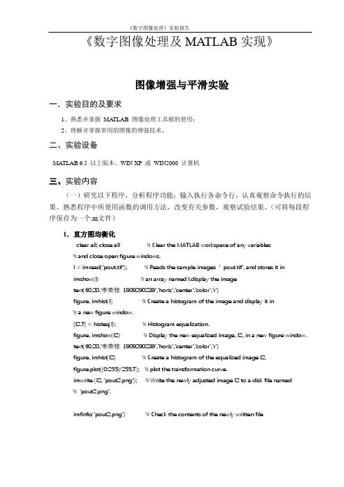
二、实验设备MATLAB 6.5 以上版本、WIN XP 或WIN2000 计算机三、实验内容（一）研究以下程序，分析程序功能；输入执行各命令行，认真观察命令执行的结果。

熟悉程序中所使用函数的调用方法，改变有关参数，观察试验结果。

（可将每段程序保存为一个.m文件）1．直方图均衡化clear all; close all % Clear the MATLAB workspace of any variables% and close open figure windows.I = imread('pout.tif'); % Reads the sample images ‘pout.tif’, and stores it inimshow(I) % an array named I.display the imagetext(60,20,'李荣桉1909290239','horiz','center','color','r')figure, imhist(I) % Create a histogram of the image and display it in% a new figure window.[I2,T] = histeq(I); % Histogram equalization.figure, imshow(I2) % Display the new equalized image, I2, in a new figure window.text(60,20,'李荣桉1909290239','horiz','center','color','r')figure, imhist(I2) % Create a histogram of the equalized image I2.figure,plot((0:255)/255,T); % plot the transformation curve.imwrite (I2, 'pout2.png'); % Write the newly adjusted image I2 to a disk file named% ‘pout2.png’.imfinfo('pout2.png') % Check the contents of the newly written file2．直接灰度变换clear all; close allI = imread('cameraman.tif'); 注意：imadjust()功能：调整图像灰度值或颜色映像表，也可实现伽马校正。