2020161自动控制原理(中英文)

自动控制原理（中英文）《自动控制原理》课程教学大纲课程编号：２020161课程类别：必修授课对象:本科三年级先修课程:复变函数，积分变换,信号与系统。

学分:4总学时:５6 课内学时:４８实验学时: ８一、课程性质、教学目得与任务课程性质:专业基础课，专业知识链条中得关键环节之一，自动控制原理就是仪器仪表类、测控类专业得重要基础课之一,这些专业主要学习信号传感(获取）、信号处理、控制及光机电系统等知识，而控制就是知识链条中得重要一环，随着科技发展，自动化、智能化已成为仪器、产品、系统等得重要功能，这就要求学生必须具备自动控制方面得知识。

教学目得与任务：培养学生自动控制原理得基础知识,学习掌握经典控制得基本理论、基本方法与控制系统得基本设计方法,重点学习分析与设计线性控制系统得基本理论、基本方法及控制系统设计方法.主要内容包括:控制系统得数学模型、控制系统得时域分析法、控制系统得根轨迹法、控制系统得频域分析法、控制系统得常用校正方法等。

二、教学基本要求学习经典控制得基本理论与基本方法,重点学习分析与设计线性控制系统得基本理论与基本方法。

主要内容包括：控制系统得数学模型、控制系统得时域分析法、控制系统得根轨迹法、控制系统得频域分析法、控制系统得常用校正方法等。

三、教学内容第一章控制系统得一般要概念 (4课时）自动控制得基本原理与方式,自动控制系统示例，自动控制系统得分类，对自动控制系统得基本要求1、基本概念;2、反馈系统基本组成；3、基本控制方式；4、控制系统分类:开环、闭环、复合控制;第二章控制系统得数学模型 (8课时）控制系统得时域数学模型,拉普拉斯变换，控制系统得复域数学模型，控制系统得状态空间模型,控制系统得结构图与信号流图２－１时域模型、微分方程表示方法;2－2 复域模型1、传递函数得定义与性质;2、传递函数得零、极点表示，开环增益、根轨迹增益等;3、典型环节得传递函数（比例、惯性、微分、积分、振荡）；2－3 控制系统得结构图与信号流图1、结构图得等效变换与化简2、信号流图组成与性质A．性质、术语（理解）B。

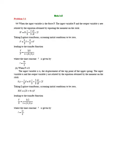
Module3Problem 3.1(a) When the input variable is the force F. The input variable F and the output variable y are related by the equation obtained by equating the moment on the stick:2.233y dylF lk c l dt=+Taking Laplace transforms, assuming initial conditions to be zero,433k F Y csY =+leading to the transfer function31(4)Y k F c k s=+ where the time constant τ is given by4c kτ=(b) When F = 0The input variable is x, the displacement of the top point of the upper spring. The input variable x and the output variable y are related by the equation obtained by the moment on the stick:2().2333y y dy k x l kl c l dt-=+Taking Laplace transforms, assuming initial conditions to be zero,3(24)kX k cs Y =+leading to the transfer function321(2)Y X c k s=+ where the time constant τ is given by2c kτ=Problem 3.2 P 54Determine the output of the open-loop systemG(s) = 1asT+to the inputr(t) = tSketch both input and output as functions of time, and determine the steady-state error between the input and output. Compare the result with that given by Fig3.7 . Solution ：While the input r(t) = t , use Laplace transforms, Input r(s)=21sOutput c(s) = r(s) G(s) = 2(1)aTs s ⋅+ = 211T T a s s Ts ⎛⎫ ⎪-+ ⎪ ⎪+⎝⎭the time-domain response becomes c(t) = ()1t Tat aT e ---Problem 3.33.3 The massless bar shown in Fig.P3.3 has been displaced a distance 0x and is subjected to a unit impulse δ in the direction shown. Find the response of the system for t>0 and sketch the result as a function of time. Confirm the steady-state response using the final-value theorem. Solution ：The equation obtained by equating the force:00()kx cxt δ+=Taking Laplace transforms, assuming initial condition to be zero,K 0X +Cs 0X =1leading to the transfer function()XF s =1K Cs +=1C1K s C+The time-domain response becomesx(t)=1CC tK e -The steady-state response using the final-value theorem:lim ()t x t →∞=0lim s →s 1K Cs +1s =1K00000()()()1;11111()K t CK x x Cx t Kx X K Cs Kx Kx X C Cs K K s KKx x t eCδ-++=⇒++=--∴==⋅++-=⋅According to the final-value theorem:0001lim ()lim lim 01t s s Kx sx t s X C K s K→∞→→-=⋅=⋅=+ Problem 3.4 Solution:1.If the input is a unit step, then1()R s s=()()11R s C s sτ−−−→−−−→+ leading to,1()(1)C s s sτ=+taking the inverse Laplace transform gives,()1tc t e τ-=-as the steady-state output is said to have been achieved once it is within 1% of the final value, we can solute ―t‖ like this,()199%1tc t e τ-=-=⨯ (the final value is 1) hence,0.014.60546.05te t sττ-==⨯=(the time constant τ=10s)2.the numerical value of the numerator of the transfer function doesn’t affect the answer. See this equation, If ()()()1C s AG s R s sτ==+ then()(1)A C s s sτ=+giving the time-domain response()(1)tc t A e τ-=-as the final value is A, the steady-state output is achieved when,()(1)99%tc t A e A τ-=-=⨯solute the equation, t=4.605τ=46.05sthe result make no different from that above, so we said that the numerical value of the numerator of the transfer function doesn’t affect the answer.If a<1, as the time increase, the two lines won`t cross. In the steady state the output lags the input by a time by more than the time constant T. The steady error will be negative infinite.R(t)C(t)Fig 3.7 tR(t)C(t)tIf a=1, as the time increase, the two lines will be parallel. It is as same as Fig 3.7.R(t)C(t)tIf a>1, as the time increase, the two lines will cross. In the steady state the output lags the input by a time by less than the time constant T.The steady error will be positive infinite.Problem 3.5 Solution: R(s)=261s s+, Y(s)=26(51)s s s +⋅+=229614551s s s -+++ /5()62929t y t t e -∴=-+so the steady-state error is 29(-30). To conform the result:5lim ()lim(62929);tt t y t t -→∞→∞=-+=∞6lim ()lim ()lim ()lim(51)t s s s s y t y s Y s s s →∞→→→+====∞+.20lim ()lim ()lim [()()]161lim [()1]()lim (1)()5130ss t s s s s e e t S E S S Y S R S S G S R S S S S S→∞→→→→==⋅=⋅-=⋅-=⋅-⋅++=- Therefore, the solution is basically correct.Problem 3.623yy x += since input is of constant amplitude and variable frequency , it can be represented as:j tX eA ω=as we know ,the output should be a sinusoidal signal with the same frequency of the input ,it can also be represented as:R(t)C(t)t0j t y y e ω=hence23j tj tj tj yyeeeA ωωωω+=00132j y Aω=+ 0294Ayω=+ 2tan3w ϕ=- Its DC(w→0) value is 003Ay ω==Requirement 01122w yy==21123294AA ω=⨯+ →32w = while phase lag of the input:1tan 14πϕ-=-=-Problem 3.7One definition of the bandwidth of a system is the frequency range over which the amplitude of the output signal is greater than 70% of the input signal amplitude when a system is subjected to a harmonic input. Find a relationship between the bandwidth and the time constant of a first-order system. What is the phase angle at the bandwidth frequency ？ Solution ：From the equation 3.41000.71r A r ωτ22=≥+ (1)and ω≥0 (2) so 1.020ωτ≤≤so the bandwidth 1.02B ωτ=from the equation 3.43the phase angle 110tan tan 1.024c πωτ--∠=-=-=Problem 3.8 3.8 SolutionAccording to generalized transfer function of First-Order Feedback Systems11C KG K RKGHK sτ==+++the steady state of the output of this system is 2.5V .∴if s →0, 2.51104C R→=. From this ,we can get the value of K, that is 13K =.Since we know that the step input is 10V , taking Laplace transforms,the input is 10S.Then the output is followed1103()113C s S s τ=⨯++Taking reverse Laplace transforms,4/4332.5 2.5 2.5(1)t t C e eττ--=-=-From the figure, we can see that when the time reached 3s,the value of output is 86% of the steady state. So we can know34823(2)*4393τττ-=-⇒-=-⇒=, 4/3310.8642t t e ττ-=-=⇒=The transfer function is3128s +146s+Let 12+8s=0, we can get the pole, that is 1.5s =-2/3- Problem 3.9 Page 55 Solution:The transfer function can be represented,()()()()()()()o o m i m i v s v s v s G s v s v s v s ==⋅While,()1()111//()()11//o m m i v s v s sRCR v s sC sC v s R R sC sC =+⎛⎫+ ⎪⎝⎭=⎡⎤⎛⎫++ ⎪⎢⎥⎝⎭⎣⎦Leading to the final transfer function,21()13()G s sRC sRC =++ And the reason:the second simple lag compensation network can be regarded as the load of the first one, and according to Load Effect , the load affects the primary relationship; so the transfer function of the comb ination doesn’t equal the product of the two individual lag transfer functio nModule4Problem4.14.1The closed-loop transfer function is10(6)102(6)101610S S S S C RS s +++++==Comparing with the generalized second-order system,we getProblem4.34.3Considering the spring rise x and the mass rise y. Using Newton ’s second law of motion..()()d x y m y K x y c dt-=-+Taking Laplace transforms, assuming zero initial conditions2mYs KX KY csX csY =-+-resulting in the transfer funcition where2Y cs K X ms cs K +=++ And521.26*10cmkc ζ== Problem4.4 Solution:The closed-loop transfer function is210263101011n n d n W EW E W W E ====-=2121212K C K S S K R S S K S S ∙+==+++∙+Comparing the closed-loop transfer function with the generalized form,2222n n nCR s s ωξωω=++ it is seen that2n K ω= And that22n ξω= ; 1Kξ=The percentage overshoot is therefore21100PO eξπξ--=11100k keπ-∙-=Where 10%PO ≤When solved, gives 1.2K ≤（2.86）When K takes the value 1.2, the poles of the system are given by22 1.20s s ++=Which gives10.45s j =-±±s=-1 1.36jProblem4.5ReIm0.45-0.45-14.5 A unity-feedback control system has the forward-path transfer functionG (s) =10)S(s K+Find the closed-loop transfer function, and develop expressions for the damping ratio And damped natural frequency in term of K Plot the closed-loop poles on the complex Plane for K = 0,10,25,50,100.For each value of K calculate the corresponding damping ratio and damped natural frequency. What conclusions can you draw from the plot?Solution: Substitute G(s)=(10)K s s + into the feedback formula : Φ(s)=()1()G S HG S +.And in unitfeedback system H=1. Result in: Φ(s)=210Ks s K++ So the damped natural frequencyn ω=K ,damping ratio ζ=102k =5k.The characteristic equation is 2s +10S+K=0. When K ≤25,s=525K -±-; While K>25,s=525i K -±-; The value ofn ω and ζ corresponding to K are listed as follows.K 0 10 25 50 100 Pole 1 1S 0 515-+ -5 -5+5i 553i -+Pole 2 2S -10 515-- -5 -5-5i553i --n ω 010 5 52 10 ζ ∞2.51 0.5 0.5Plot the complex plane for each value of K:We can conclude from the plot.When k ≤25,poles distribute on the real axis. The smaller value of K is, the farther poles is away from point –5. The larger value of K is, the nearer poles is away from point –5.When k>25,poles distribute away from the real axis. The smaller value of K is, the further (nearer) poles is away from point –5. The larger value of K is, the nearer (farther) poles is away from point –5.And all the poles distribute on a line parallels imaginary axis, intersect real axis on the pole –5.Problem4.61tb b R L C b o v dv i i i i v dt C R L dt=++=++⎰Taking Laplace transforms, assuming zero initial conditions, reduces this equation to011b I Cs V R Ls ⎛⎫=++ ⎪⎝⎭20b V RLs I Ls R RLCs =++ Since the input is a constant current i 0, so01I s=then,()2b RLC s V Ls R RLCs==++ Applying the final-value theorem yields ()()0lim lim 0t s c t sC s →∞→==indicating that the steady-state voltage across the capacitor C eventually reaches the zero ,resulting in full error.Problem4.74.7 Prove that for an underdamped second-order system subject to a step input, thepercentage overshoot above the steady-state output is a function only of the damping ratio .Fig .4.7SolutionThe output can be given by222222()(2)21()(1)n n n n n n C s s s s s s s ωζωωζωζωωζ=+++=-++- (1)the damped natural frequencyd ω can be defined asd ω=21n ωζ- (2)substituting above results in22221()()()n n n d n d s C s s s s ζωζωζωωζωω+=--++++ (3) taking the inverse transform yields22()1sin()11tan n t d e c t t where ζωωφζζφζ-=-+--=(4)the maximum output is22()1sin()11n t p d p p d n e c t t t ζωωφζππωωζ-=-+-==-(5)so the maximum is2/1()1p c t eπζζ--=+the percentage overshoot is therefore2/1100PO eπζζ--=Problem4.8 Solution to 4.8:Considering the mass m displaced a distance x from its equilibrium position, the free-body diagram of the mass will be as shown as follows.aP cdx kxkxmUsing Newton ’s second law of motion,22p k x c x mx m x c x k x p--=++=Taking Laplace transforms, assuming zero initial conditions,2(2)X ms cs k P ++= results in the transfer function2/(1/)/((/)2/)X P m s c m s k m =++ 2(2/)(2/)((/)2/)k k m s c m s k m =++As we see2(2)X m s c s k P++= As P is constantSo X ∝212ms cs k ++ . When 56.25102cs m-=-=-⨯ ()25min210mscs k ++=4max5100.110X == This is a second-order transfer function where 22/n k m ω= and/2/22n c w m c k m ζ== The damped natural frequency is given by 2212/1/8d n k m c km ωωζ=-=-22/(/2)k m c m =- Using the given data,462510/2100.050.2236n ω=⨯⨯⨯== 462502.79501022100.05ζ-==⨯⨯⨯⨯ ()240.22361 2.7950100.2236d ω-=⨯-⨯= With these data we can draw a picture14.0501160004.673600p de s e T T πωτζωτ======222222112/1222()22,,,428sin (sin cos )0tan 7.030.02n n pp dd n dd n ntd d t t t n d p d d p ddd p p p nX k m c k P ms cs k k m s s s m m k c k c cm m m m km p x e tm p xe t t m t t x m ζωζωωωζωωωωζζωωωζωωωωωωωζω--===⋅=⋅++++++=-===∴==-+=∴=⇒=⇒= 其中Problem4.10 4.10 solution:The system is similar to the one in the book on PAGE 58 to PAGE 63. The difference is the connection of the spring. So the transfer function is2222l n d n n w s w s w θθζ=++222(),;p a m ld a m p m l m l l m mm l lk k k N RJs RCs R k k N k J N J J C N c c N N N θθωθωθ=+++=+=+===p a mn K K K w NJ R='damping ratio 2p a m c NRK K K J ζ='But the value of J is different, because there is a spring connected.122s m J J J J N N '=++Because of final-value theorem,2l nd w θθζ=Module5Problem5.45．4 The closed-loop transfer function of the system may be written as2221010(1)610101*********CR K K K S S K K S S K S S +++==+++++++ The closed-loop poles are the solutions of the characteristic equation6364(1010)3110210(1)n K S K JW K -±-+==-±+=+ 210(1)6310(1)E K E K +==+In order to study the stability of the system, the behavior of the closed-loop poles when the gain K increases from zero to infinte will be observed. So when12K = 3010E =321S J =-± 210K = 3110110E =3101S J =-± 320K = 21070E =3201S J =-±双击下面可以看到原图ReProblem5.5SolutionThe closed-loop transfer function is2222(1)1(1)KC K KsKR s K as s aKs Kass===+++++∙+Comparing the closed-loop transfer function with the generalized form, 2222nn nCR s sωξωω=++Leading to2nKa Kωξ==The percentage overshoot is therefore2110040%PO eξπξ--==Producing the result0.869ξ=（0.28）And the peak time241PnT sπωξ==-Leading to1.586nω=（0.82）Problem5.75.7 Prove that the rise time T r of a second-order system with a unit step input is given byT r = d ω1 tan -1n dζωω = d ω1 tan -1d ωζ21--Plot the rise against the damping ratio.Solution:According to (4.33):c(t)=1-2(cos sin )1n t d d e t t ζωζωωζ-+-. 4.33When t=r T ,c(t)=1.substitue c(t)= 1 into (4.33) Producing the resultr T =d ω1 tan -1n dζωω = d ω1 tan -112ζζ--Plot the rise time against the damping ratio:Problem5.9Solution to 5.9:As we know that the system is the open-loop transfer function of a unity-feedback control system.So ()()GH S G S = Given as()()()425KGH s s s =-+The close-loop transfer function of the system may be written as()()()()()41254G s C Ks R GH s s s K ==+-++ The characteristic equation is()()2254034100s s K s s K -++=⇒++-=According to the Routh ’s method, the Routh ’s array must be formed as follow20141030410s K s s K -- For there is no closed-loop poles to the right of the imaginary axis4100 2.5K K -≥⇒≥ Given that 0.5ζ=4103 4.752410n K K K ωζ=-=⇒=- When K=0, the root are s=+2,-5According to the characteristic equation, the solutions are349424s K =-±-while 3.0625K ≤, we have one or two solutions, all are integral number.Or we will have solutions with imaginary number. So we can drawK=102 -5 K=0K=3.0625K=2.5 K=10Open-loop polesClosed-loop polesProblem5.10 5.10 solution:0.62/n w rad sζ==according to()211sin()21n w t d e c w t ζφζ-=-+=- 1.2sin(1.6)0.4t e t φ-⋅+= 4t a n3φ= finally, t is delay time:1.23t s ≈(0.67)Module6Problem 6.3First we assume the disturbance D to be zero:e R C =-1011C K e s s =⋅⋅⋅+Hence:(1)10(1)e s s R K s s +=++ Then we set the input R to be zero:10()(1)C K e D e s s =⋅+⋅=-+ ⇒ 1010(1)e D K s s =-++Adding these two results together:(1)1010(1)10(1)s s e R D K s s K s s +=⋅-⋅++++21()R s s =; 1()D s s= ∴222110910(1)10(1)100(1)s s e Ks s s Ks s s s s s +-=-=++++++ the steady-state error:232200099lim lim lim 0.09100100ss s s s s s s e s e s s s s s →→→--=⋅===-++++Problem 6.4Determine the disturbance rejection ratio(DRR) for the system shown in Fig P.6.4+fig.P.6.4 solution ：from the diagram we can know :0.210.05mv K RK c === so we can get that()0.21115()0.05v m m OL n CL K K DRR cR ωω∆⨯==+=+=∆210.10.050.050.025s s =++, so c=0.025, DRR=9Problem 6.5 6.5 SolutionFor the purposes of determining the steady-state error of the system, we should get to know the effect of the input and the disturbance along when the other will be assumed to be zero.First to simplify the block diagram to the following patter:110s +2021Js Tddθoθ0.220.10.05s ++__+d T—Allowing the transfer function from the input to the output position to be written as01220220d Js s θθ=++ 012222020240*220220(220)dJs s Js s s Js s sθθ===++++++ According to the equation E=R-C:022*******(2)()lim[()()]lim[(1)]lim 0.2220220ssr d s s s Js e s s s s Js s Js s δδδθθ→→→+=-=-==++++问题;1. 系统型为2，对于阶跃输入，稳态误差为0.2. 终值定理写的不对。

自动控制原理（B）课程简介课程编号：15J8047课程名称：（中文）自动控制原理（B）（英文）Introduction to Automatic Control学分/学时：42学时，实验6学时开课学期：秋季先修课程：高等数学、工程数学、大学物理内容简介：（500字以内）《自动控制原理》属于技术科学，是为专业课学习和参加控制工程实践而设置的，研究的对象是自动控制系统，研究的中心问题是控制系统在控制过程中的性能，学科的基本内容分为数学模型、工程分析计算方法和系统一般规律三个部分。

要求学生能够正确地理解和运用课程的基本概念及基本理论，逐步掌握“定性分析、定量估算和仿真实验"的研究问题的方法。

本课程内容主要为经典控制中的线性理论，课程前后内容联系紧密、系统性强，所附加的实验课，以学习控制系统的基本实验方法和培养测试、分析能力为主。

自动控制原理（B）课程教学大纲课程编号：15J8047课程名称：（中文）自动控制原理（B）（英文）Introduction to Automatic Control学分/学时：42学时，实验6学时先修课程：高等数学、工程数学、大学物理课程教学目标课程的性质：本科专业基本课，为必修课目的和任务：本课程是研究自动控制系统规律性的一门工程学科，是重要的专业基本课程。

通过本课程的教学工作，要求学生能够正确地理解和运用课程的基本概念和理论，逐步掌握“定性分析、定量估算和仿真实验”的研究问题的方法，具有从事与飞行器自动控制系统有■关的丁程实践与理论研究的基本知识，并为进一步学习现代控制理论打下基本。

教学内容及基本要求第一章自动控制的一般概念（2学时）1.1自动控制的任务1.2自动控制的基本方式1.3自动控制系统示例1.4对控制系统的性能要求第二章自动控制系统的数学模型（8学时）2.1控制系统微分方程的建立2.2非线性微分方程的线性化2.3拉普拉斯变换2.4传递函数2.5动态结构图2.6结构图的等效变换2.7典型反馈系统的几种传递函数第三章时域分析法（8学时）3.1典型响应及性能指标3.2 一、二阶系统分析3.3二阶系统分析3.4系统稳态误差分析及计算第四章根轨迹法（6学时）4.1根轨迹与根轨迹方程4.2根轨迹的绘制法则4.3系统闭环零、极点分布与阶跃响应的关系4.4系统阶跃响应的根轨迹分析第五章频率法（8学时）5.1频率特性5.2典型环节的频率特性5.3开环系统的频率特性5.4频率稳定判据5.5系统闭环频率特性与阶跃响应的关系5.5开环频率特性与系统阶跃响应的关系第六章控制系统的校正方法（4学时）6.1系统校正设计基础6.2串联校正6.3串联校正的理论设计方法6.4反馈校正6.5复合校正第七章状态空间分析方法（6学时）7.1状态空间方法基础7.2线性系统的可控性和可观测性7.3状态反馈与状态观测器7.4有界输入、有界输出稳定性7.5李雅普诺夫第二方法.教学安排及方式学时分配：讲课实验习题课第一章21第二章82第三章821第四章61第五章821第六章421第七章6课内外学时比：1:1.5实验安排：共三次实验，每次二小时。

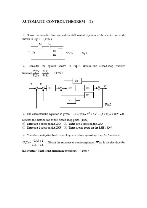
AUTOMATIC CONTROL THEOREM (1)⒈ Derive the transfer function and the differential equation of the electric network⒉ Consider the system shown in Fig.2. Obtain the closed-loop transfer function)()(S R S C , )()(S R S E . （12%） ⒊ The characteristic equation is given 010)6(5)(123=++++=+K S K S S S GH . Discuss the distribution of the closed-loop poles. (16%)① There are 3 roots on the LHP ② There are 2 roots on the LHP② There are 1 roots on the LHP ④ There are no roots on the LHP . K=?⒋ Consider a unity-feedback control system whose open-loop transfer function is )6.0(14.0)(++=S S S S G . Obtain the response to a unit-step input. What is the rise time for this system? What is the maximum overshoot? （10%）Fig.15. Sketch the root-locus plot for the system )1()(+=S S K S GH . ( The gain K is assumed to be positive.)① Determine the breakaway point and K value.② Determine the value of K at which root loci cross the imaginary axis.③ Discuss the stability. (12%)6. The system block diagram is shown Fig.3. Suppose )2(t r +=, 1=n . Determine the value of K to ensure 1≤e . (12%)Fig.37. Consider the system with the following open-loop transfer function:)1)(1()(21++=S T S T S K S GH . ① Draw Nyquist diagrams. ② Determine the stability of the system for two cases, ⑴ the gain K is small, ⑵ K is large. (12%)8. Sketch the Bode diagram of the system shown in Fig.4. (14%)⒈212121121212)()()(C C S C C R R C S C C R S V S V ++++=⒉ 2423241321121413211)()(H G H G G G G G G G H G G G G G G G S R S C ++++++=⒊ ① 0<K<6 ② K ≤0 ③ K ≥6 ④ no answer⒋⒌①the breakaway point is –1 and –1/3; k=4/27 ② The imaginary axis S=±j; K=2③⒍5.75.3≤≤K⒎ )154.82)(181.34)(1481.3)(1316.0()11.0(62.31)(+++++=S S S S S S GHAUTOMATIC CONTROL THEOREM (2)⒈Derive the transfer function and the differential equation of the electric network⒉ Consider the equation group shown in Equation.1. Draw block diagram and obtain the closed-loop transfer function )()(S R S C . （16% ） Equation.1 ⎪⎪⎩⎪⎪⎨⎧=-=-=--=)()()()()]()()([)()]()()()[()()()]()()[()()()(3435233612287111S X S G S C S G S G S C S X S X S X S G S X S G S X S C S G S G S G S R S G S X⒊ Use Routh ’s criterion to determine the number of roots in the right-half S plane for the equation 0400600226283)(12345=+++++=+S S S S S S GH . Analyze stability.（12% ）⒋ Determine the range of K value ,when )1(2t t r ++=, 5.0≤SS e . （12% ）Fig.1⒌Fig.3 shows a unity-feedback control system. By sketching the Nyquist diagram of the system, determine the maximum value of K consistent with stability, and check the result using Routh ’s criterion. Sketch the root-locus for the system （20%）（18% ）⒎ Determine the transfer function. Assume a minimum-phase transfer function.（10% ）⒈1)(1)()(2122112221112++++=S C R C R C R S C R C R S V S V⒉ )(1)()(8743215436324321G G G G G G G G G G G G G G G G S R S C -+++=⒊ There are 4 roots in the left-half S plane, 2 roots on the imaginary axes, 0 root in the RSP. The system is unstable.⒋ 208<≤K⒌ K=20⒍⒎ )154.82)(181.34)(1481.3)(1316.0()11.0(62.31)(+++++=S S S S S S GHAUTOMATIC CONTROL THEOREM (3)⒈List the major advantages and disadvantages of open-loop control systems. (12% )⒉Derive the transfer function and the differential equation of the electric network⒊ Consider the system shown in Fig.2. Obtain the closed-loop transfer function)()(S R S C , )()(S R S E , )()(S P S C . （12%）⒋ The characteristic equation is given 02023)(123=+++=+S S S S GH . Discuss the distribution of the closed-loop poles. (16%)5. Sketch the root-locus plot for the system )1()(+=S S K S GH . (The gain K is assumed to be positive.)④ Determine the breakaway point and K value.⑤ Determine the value of K at which root loci cross the imaginary axis. ⑥ Discuss the stability. (14%)6. The system block diagram is shown Fig.3. 21+=S K G , )3(42+=S S G . Suppose )2(t r +=, 1=n . Determine the value of K to ensure 1≤SS e . (15%)7. Consider the system with the following open-loop transfer function:)1)(1()(21++=S T S T S K S GH . ① Draw Nyquist diagrams. ② Determine the stability of the system for two cases, ⑴ the gain K is small, ⑵ K is large. (15%)⒈ Solution: The advantages of open-loop control systems are as follows: ① Simple construction and ease of maintenance② Less expensive than a corresponding closed-loop system③ There is no stability problem④ Convenient when output is hard to measure or economically not feasible. (For example, it would be quite expensive to provide a device to measure the quality of the output of a toaster.)The disadvantages of open-loop control systems are as follows:① Disturbances and changes in calibration cause errors, and the output may be different from what is desired.② To maintain the required quality in the output, recalibration is necessary from time to time.⒉ 1)(1)()()(2122112221122112221112+++++++=S C R C R C R S C R C R S C R C R S C R C R S U S U ⒊351343212321215143211)()(H G G H G G G G H G G H G G G G G G G G S R S C +++++= 35134321232121253121431)1()()(H G G H G G G G H G G H G G H G G H G G G G S P S C ++++-+=⒋ R=2, L=1⒌ S:①the breakaway point is –1 and –1/3; k=4/27 ② The imaginary axis S=±j; K=2⒍5.75.3≤≤KAUTOMATIC CONTROL THEOREM (4)⒈ Find the poles of the following )(s F :se s F --=11)( (12%)⒉Consider the system shown in Fig.1,where 6.0=ξ and 5=n ωrad/sec. Obtain the rise time r t , peak time p t , maximum overshoot P M , and settling time s t when the system is subjected to a unit-step input. （10%）⒊ Consider the system shown in Fig.2. Obtain the closed-loop transfer function)()(S R S C , )()(S R S E , )()(S P S C . （12%）⒋ The characteristic equation is given 02023)(123=+++=+S S S S GH . Discuss the distribution of the closed-loop poles. (16%)5. Sketch the root-locus plot for the system )1()(+=S S K S GH . (The gain K is assumed to be positive.)⑦ Determine the breakaway point and K value.⑧ Determine the value of K at which root loci cross the imaginary axis.⑨ Discuss the stability. (12%)6. The system block diagram is shown Fig.3. 21+=S K G , )3(42+=S S G . Suppose )2(t r +=, 1=n . Determine the value of K to ensure 1≤SS e . (12%)7. Consider the system with the following open-loop transfer function:)1)(1()(21++=S T S T S K S GH . ① Draw Nyquist diagrams. ② Determine the stability of the system for two cases, ⑴ the gain K is small, ⑵ K is large. (12%)8. Sketch the Bode diagram of the system shown in Fig.4. (14%)⒈ Solution: The poles are found from 1=-s e or 1)sin (cos )(=-=-+-ωωσωσj e e j From this it follows that πωσn 2,0±== ),2,1,0( =n . Thus, the poles are located at πn j s 2±=⒉Solution: rise time sec 55.0=r t , peak time sec 785.0=p t ,maximum overshoot 095.0=P M ,and settling time sec 33.1=s t for the %2 criterion, settling time sec 1=s t for the %5 criterion.⒊ 351343212321215143211)()(H G G H G G G G H G G H G G G G G G G G S R S C +++++= 35134321232121253121431)1()()(H G G H G G G G H G G H G G H G G H G G G G S P S C ++++-+=⒋R=2, L=15. S:①the breakaway point is –1 and –1/3; k=4/27 ② The imaginary axis S=±j; K=2⒍5.75.3≤≤KAUTOMATIC CONTROL THEOREM (5)⒈ Consider the system shown in Fig.1. Obtain the closed-loop transfer function )()(S R S C , )()(S R S E . （18%）⒉ The characteristic equation is given 0483224123)(12345=+++++=+S S S S S S GH . Discuss the distribution of the closed-loop poles. (16%)⒊ Sketch the root-locus plot for the system )15.0)(1()(++=S S S K S GH . (The gain K is assumed to be positive.)① Determine the breakaway point and K value.② Determine the value of K at which root loci cross the imaginary axis. ③ Discuss the stability. (18%)⒋ The system block diagram is shown Fig.2. 1111+=S T K G , 1222+=S T K G . ①Suppose 0=r , 1=n . Determine the value of SS e . ②Suppose 1=r , 1=n . Determine the value of SS e . (14%)⒌ Sketch the Bode diagram for the following transfer function. )1()(Ts s K s GH +=, 7=K , 087.0=T . (10%)⒍ A system with the open-loop transfer function )1()(2+=TS s K S GH is inherently unstable. This system can be stabilized by adding derivative control. Sketch the polar plots for the open-loop transfer function with and without derivative control. (14%)⒎ Draw the block diagram and determine the transfer function. (10%)⒈∆=321)()(G G G S R S C ⒉R=0, L=3,I=2⒋①2121K K K e ss +-=②21211K K K e ss +-= ⒎11)()(12+=RCs s U s UAUTOMATIC CONTROL THEOREM (6)⒈ Consider the system shown in Fig.1. Obtain the closed-loop transfer function )()(S R S C , )()(S R S E . （18%）⒉The characteristic equation is given 012012212010525)(12345=+++++=+S S S S S S GH . Discuss thedistribution of the closed-loop poles. (12%)⒊ Sketch the root-locus plot for the system )3()1()(-+=S S S K S GH . (The gain K is assumed to be positive.)① Determine the breakaway point and K value.② Determine the value of K at which root loci cross the imaginary axis. ③ Discuss the stability. (15%)⒋ The system block diagram is shown Fig.2. SG 11=, )125.0(102+=S S G . Suppose t r +=1, 1.0=n . Determine the value of SS e . (12%)⒌ Calculate the transfer function for the following Bode diagram of the minimum phase. (15%)⒍ For the system show as follows, )5(4)(+=s s s G ,1)(=s H , (16%) ① Determine the system output )(t c to a unit step, ramp input.② Determine the coefficient P K , V K and the steady state error to t t r 2)(=.⒎ Plot the Bode diagram of the system described by the open-loop transfer function elements )5.01()1(10)(s s s s G ++=, 1)(=s H . (12%)w⒈32221212321221122211)1()()(H H G H H G G H H G G H G H G H G G G S R S C +-++-+-+= ⒉R=0, L=5 ⒌)1611()14)(1)(110(05.0)(2s s s s s s G ++++= ⒍t t e e t c 431341)(--+-= t t e e t t c 41213445)(---+-= ∞=P K , 8.0=V K , 5.2=ss eAUTOMATIC CONTROL THEOREM (7)⒈ Consider the system shown in Fig.1. Obtain the closed-loop transfer function)()(S R S C , )()(S R S E . （16%）⒉ The characteristic equation is given 01087444)(123456=+--+-+=+S S S S S S S GH . Discuss the distribution of the closed-loop poles. (10%)⒊ Sketch the root-locus plot for the system 3)1()(S S K S GH +=. (The gain K is assumed to be positive.)① Determine the breakaway point and K value.② Determine the value of K at which root loci cross the imaginary axis. ③ Discuss the stability. (15%)⒋ Show that the steady-state error in the response to ramp inputs can be made zero, if the closed-loop transfer function is given by:nn n n n n a s a s a s a s a s R s C +++++=---1111)()( ;1)(=s H （12%）⒌ Calculate the transfer function for the following Bode diagram of the minimum phase.（15%）w⒍ Sketch the Nyquist diagram (Polar plot) for the system described by the open-loop transfer function )12.0(11.0)(++=s s s S GH , and find the frequency and phase such that magnitude is unity. （16%）⒎ The stability of a closed-loop system with the following open-loop transfer function )1()1()(122++=s T s s T K S GH depends on the relative magnitudes of 1T and 2T . Draw Nyquist diagram and determine the stability of the system.（16%） ( 00021>>>T T K )⒈3213221132112)()(G G G G G G G G G G G G S R S C ++-++=⒉R=2, I=2,L=2 ⒌)1()1()(32122++=ωωωs s s s G⒍o s rad 5.95/986.0-=Φ=ωAUTOMATIC CONTROL THEOREM (8)⒈ Consider the system shown in Fig.1. Obtain the closed-loop transfer function)()(S R S C , )()(S R S E . （16%）⒉ The characteristic equation is given 04)2(3)(123=++++=+S K KS S S GH . Discuss the condition of stability. (12%)⒊ Draw the root-locus plot for the system 22)4()1()(++=S S KS GH ;1)(=s H .Observe that values of K the system is overdamped and values of K it is underdamped. (16%)⒋ The system transfer function is )1)(21()5.01()(s s s s K s G +++=,1)(=s H . Determine thesteady-state error SS e when input is unit impulse )(t δ、unit step )(1t 、unit ramp t and unit parabolic function221t . (16%)⒌ ① Calculate the transfer function (minimum phase);② Draw the phase-angle versus ω (12%) w⒍ Draw the root locus for the system with open-loop transfer function.)3)(2()1()(+++=s s s s K s GH (14%)⒎ )1()(3+=Ts s Ks GH Draw the polar plot and determine the stability of system. (14%)⒈43214321432143211)()(G G G G G G G G G G G G G G G G S R S C -+--+= ⒉∞ K 528.0⒊S:0<K<0.0718 or K>14 overdamped ;0.0718<K<14 underdamped⒋S: )(t δ 0=ss e ; )(1t 0=ss e ; t K e ss 1=; 221t ∞=ss e⒌S:21ωω=K ; )1()1()(32121++=ωωωωs s ss GAUTOMATIC CONTROL THEOREM (9)⒈ Consider the system shown in Fig.1. Obtain the closed-loop transfer function)(S C , )(S E . （12%）⒉ The characteristic equation is given0750075005.34)(123=+++=+K S S S S GH . Discuss the condition of stability. (16%)⒊ Sketch the root-locus plot for the system )1(4)()(2++=s s a s S GH . (The gain a isassumed to be positive.)① Determine the breakaway point and a value.② Determine the value of a at which root loci cross the imaginary axis. ③ Discuss the stability. (12%)⒋ Consider the system shown in Fig.2. 1)(1+=s K s G i , )1()(2+=Ts s Ks G . Assumethat the input is a ramp input, or at t r =)( where a is an arbitrary constant. Show that by properly adjusting the value of i K , the steady-state error SS e in the response to ramp inputs can be made zero. (15%)⒌ Consider the closed-loop system having the following open-loop transfer function:)1()(-=TS S KS GH . ① Sketch the polar plot ( Nyquist diagram). ② Determine thestability of the closed-loop system. (12%)⒍Sketch the root-locus plot. (18%)⒎Obtain the closed-loop transfer function )()(S R S C . （15%）⒈354211335421243212321313542143211)1()()(H G G G G H G H G G G G H G G G G H G G H G H G G G G G G G G G S R S C --++++-= 354211335421243212321335422341)()(H G G G G H G H G G G G H G G G G H G G H G H G G G H H G S N S E --+++--= ⒉45.30 K⒌S: N=1 P=1 Z=0; the closed-loop system is stable ⒎2423241321121413211)()(H G H G G G G G G G H G G G G G G G S R S C ++++++=AUTOMATIC CONTROL THEOREM (10)⒈ Consider the system shown in Fig.1. Obtain the closed-loop transfer function)()(S R S C ,⒉ The characteristic equation is given01510520)(1234=++++=+S S KS S S GH . Discuss the condition of stability. (14%)⒊ Consider a unity-feedback control system whose open-loop transfer function is)6.0(14.0)(++=S S S S G . Obtain the response to a unit-step input. What is the rise time forthis system? What is the maximum overshoot? （10%）⒋ Sketch the root-locus plot for the system )25.01()5.01()(s S s K S GH +-=. (The gain K isassumed to be positive.)③ Determine the breakaway point and K value.④ Determine the value of K at which root loci cross the imaginary axis. Discuss the stability. (15%)⒌ The system transfer function is )5(4)(+=s s s G ,1)(=s H . ①Determine thesteady-state output )(t c when input is unit step )(1t 、unit ramp t . ②Determine theP K 、V K and a K , obtain the steady-state error SS e when input is t t r 2)(=. （12%）⒍ Consider the closed-loop system whose open-loop transfer function is given by:①TS K S GH +=1)(; ②TS K S GH -=1)(; ③1)(-=TS KS GH . Examine the stabilityof the system. （15%）⒎ Sketch the root-locus plot 。

《自动控制原理》部分中英文词汇对照表AAcceleration 加速度Angle of departure分离角Asymptotic stability渐近稳定性Automation自动化Auxiliary equation辅助方程BBacklash间隙Bandwidth带宽Block diagram方框图Bode diagram波特图CCauchy’s theorem高斯定理Characteristic equation特征方程Closed-loop control system闭环控制系统Constant常数Control system控制系统Controllability可控性Critical damping临界阻尼DDamping constant阻尼常数Damping ratio阻尼比DC control system直流控制系统Dead zone死区Delay time延迟时间Derivative control 微分控制Differential equations微分方程Digital computer compensator数字补偿器Dominant poles主导极点Dynamic equations动态方程EError coefficients误差系数Error transfer function误差传递函数FFeedback反馈Feedback compensation反馈补偿Feedback control systems反馈控制系统Feedback signal反馈信号Final-value theorem终值定理Frequency-domain analysis频域分析Frequency-domain design频域设计Friction摩擦GGain增益Generalized error coefficients广义误差系数IImpulse response脉冲响应Initial state初始状态Initial-value theorem初值定理Input vector输入向量Integral control积分控制Inverse z-transformation反Z变换JJordan block约当块Jordan canonical form约当标准形LLag-lead controller滞后-超前控制器Lag-lead network 滞后-超前网络Laplace transform拉氏变换Lead-lag controller超前-滞后控制器Linearization线性化Linear systems线性系统MMass质量Mathematical models数学模型Matrix矩阵Mechanical systems机械系统NNatural undamped frequency自然无阻尼频率Negative feedback负反馈Nichols chart尼科尔斯图Nonlinear control systems非线性控制系统Nyquist criterion柰奎斯特判据OObservability可观性Observer观测器Open-loop control system开环控制系统Output equations输出方程Output vector输出向量PParabolic input抛物线输入Partial fraction expansion部分分式展开PD controller比例微分控制器Peak time峰值时间Phase-lag controller相位滞后控制器Phase-lead controller相位超前控制器Phase margin相角裕度PID controller比例、积分微分控制器Polar plot极坐标图Poles definition极点定义Positive feedback正反馈Prefilter 前置滤波器Principle of the argument幅角原理RRamp error constant斜坡误差常数Ramp input斜坡输入Relative stability相对稳定性Resonant frequency共振频率Rise time上升时间调节时间 accommodation timeRobust system鲁棒系统Root loci根轨迹Routh tabulation（array）劳斯表SSampling frequency采样频率Sampling period采样周期Second-order system二阶系统Sensitivity灵敏度Series compensation串联补偿Settling time调节时间Signal flow graphs信号流图Similarity transformation相似变换Singularity奇点Spring弹簧Stability稳定性State diagram状态图State equations状态方程State feedback状态反馈State space状态空间State transition equation状态转移方程State transition matrix状态转移矩阵State variables状态变量State vector状态向量Steady-state error稳态误差Steady-state response稳态响应Step error constant阶跃误差常数Step input阶跃输入TTime delay时间延迟Time-domain analysis时域分析Time-domain design时域设计Time-invariant systems时不变系统Time-varying systems时变系统Type number型数Torque constant扭矩常数Transfer function转换方程Transient response暂态响应Transition matrix转移矩阵UUnit step response单位阶跃响应VVandermonde matrix范德蒙矩阵Velocity control system速度控制系统Velocity error constant速度误差常数ZZero-order hold零阶保持z-transfer function Z变换函数z-transform Z变换。

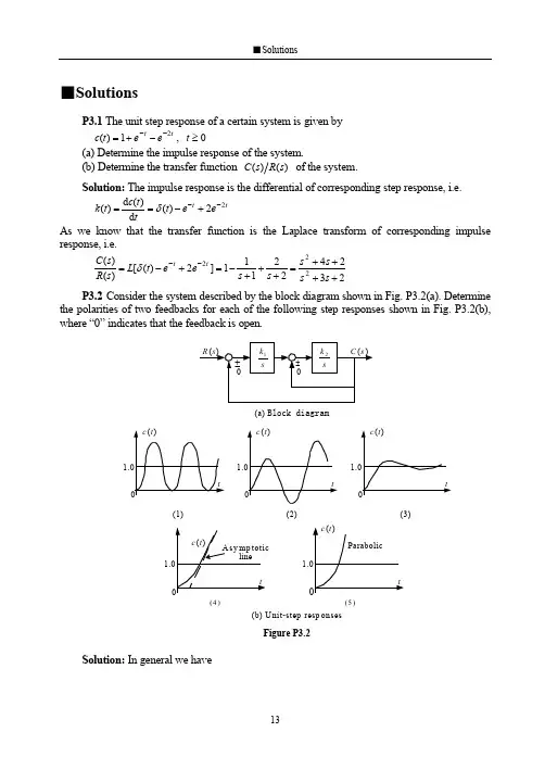
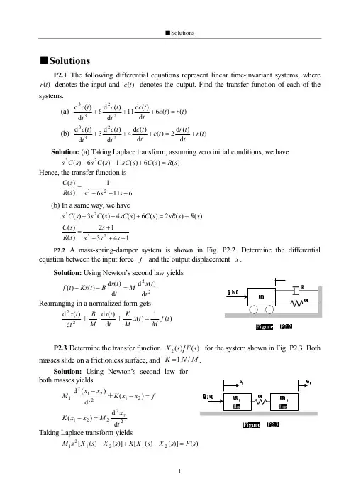
■SolutionsP3.1 The unit step response of a certain system is given by t t e e t c 21)(---+=, 0≥t (a) Determine the impulse response of the system.(b) Determine the transfer function )()(s R s C of the system.Solution:The impulse response is the differential of corresponding step response, i.e.t t e e t tt c t k 22)(d )(d )(--+-==δAs we know that the transfer function is the Laplace transform of corresponding impulse response, i.e.232422111]2)([)()(222++++=+++-=+-=--s s s s s s e e t L s R s C tt δP3.2Consider the system described by the block diagram shown in Fig. P3.2(a). Determinethe polarities of two feedbacks for each of the following step responses shown in Fig. P3.2(b), where “0” indicates that the feedback is open.Solution:In general we have(a) Block diagram.1.1.1.1.1(b) U nit-step resp onses(1)(2)(3)(4)(5)Figure P3.221020221)()(k k s k s k k s R s C ±±=Note that the characteristic polynomial is210202)(k k s k s s ±±=∆where the sign of s k 2is depended on the outer feedback and the sign of 21k k is depended on the inter feedback.Case (1).The response presents a sinusoidal. It means that the system has a pair of pure imaginary roots, i.e. the characteristic polynomial is in the form of 212)(k k s s +=∆. Obviously, the outlet feedback is “–”and the inner feedback is “0”.Case (2).The response presents a diverged oscillation.The system has a pair of complex conjugate roots with positive real parts, i.e. the characteristic polynomial is in the form of 2122)(k k s k s s +-=∆. Obviously, the outlet feedback is “+”and the inner feedback is “–”.Case (3).The response presents a converged oscillation. It means that the system has a pair of complex conjugate roots with negative real parts, i.e. the characteristic polynomial is in the form of 2122)(k k s k s s ++=∆. Obviously,both the outlet and inner feedbacks are “–”.Case (4).In fact this is a ramp response of a first-order system. Hence, the outlet feedback is “0”to produce a ramp signal and the inner feedback is “–”.Case (5).Considering that a parabolic function is the integral of a ramp function, both the outlet and inner feedbacks are “0”.P3.3Consider each of the following closed-loop transfer function. By considering the location of the poles on the complex plane, sketch the unit step response, explaining the results obtained.(a) 201220)(2++=s s s Φ,(b) 61166)(23+++=s s s s Φ(c) 224)(2++=s s s Φ,(d) )5)(52(5.12)(2+++=s s s s ΦSolution:(a) )10)(2(20201220)(2++=++=s s s s s ΦBy inspection, the characteristic roots are 2-, 10-. This is an overdamped second-order system. Therefore, considering that the closed-loop gain is 1=Φk , its unit step response can be sketched as shown.(b) )3)(2)(1(661166)(23+++=+++=s s s s s s s ΦBy inspection, the characteristic roots are 1-, 2-, 3-.Obviously, all three transient components are decayed exponential terms. Therefore, its unit step response, with a closed-loop gain 1=Φk , is sketched as shown..1.1(c) 1)1(4224)(22++=++=s s s s ΦThis is an underdamped second-order system, because its characteristic roots are j ±-1. Hence, transient component is a decayed sinusoid. Noting that the closed-loop gain is 2=Φk , the unit step response can be sketched as shown.(d) )5](21[(5.12)5)(52(5.12)(222++=+++=s s s s s s ）＋ΦBy inspection, the characteristic roots are 21j ±-, 5-. Since51.0-<<-, there is a pair of dominant poles,21j ±-, for this system. The unit step response, with a closed-loop gain 5.0=Φk , is sketched as shown.P3.4 The open-loop transfer function of a unity negative feedback system is)1(1)(+=s s s G Determine the rise time, peak time, percent overshoot and setting time (using a 5% setting criterion).Solution: Writing he closed-loop transfer function2222211)(nn n s s s s s ωςωωΦ++=++=we get 1=n ω, 5.0=ς. Since this is an underdamped second-order system with 5.0=ς, the system performance can be estimated as follows.Rising time .sec 42.25.0115.0arccos 1arccos 22≈-⋅-=--=πςωςπn r t Peak time .sec 62.35.011122≈-⋅=-=πςωπn p t Percent overshoot %3.16%100%100225.015.01≈⨯=⨯=--πςπςσe e p Setting time .sec 615.033=⨯=≈ns t ςω(using a 5% setting criterion)P3.5 A second-order system gives a unit step response shown in Fig. P3.5. Find the open-loop transfer function if the system is a unit negative-feedback system.Solution:By inspection we have%30%100113.1=⨯-=p σSolving the formula for calculating the overshoot,.1.1Figure P3.5.0.23.021==-ςπςσe p , we have 362.0ln ln 22≈+-=ppσπσςSince .sec 1=p t , solving the formula for calculating the peak time, 21ςωπ-=n p t , we getsec/7.33rad n =ωHence, the open-loop transfer function is)4.24(7.1135)2()(2+=+=s s s s s G n n ςωωP3.6A feedback system is shown in Fig. P3.6(a), and its unit step response curve is shown in Fig. P3.6(b). Determine the values of 1k , 2k ,and a .Solution:The transfer function between the input and output is given by2221)()(k as s k k s R s C ++=The system is stable and we have, from the response curve,21lim )(lim 122210==⋅++⋅=→∞→k sk as s k k s t c s t By inspection we have%9%10000.211.218.2=⨯-=p σSolving the formula for calculating the overshoot, 09.021==-ςπςσe p , we have608.0ln ln 22≈+-=ppσπσςSince .sec 8.0=p t , solving the formula for calculating the peak time, 21ςωπ-=n p t , we getsec/95.4rad n =ωThen, comparing the characteristic polynomial of the system with its standard form, we have.2.2(a)(b)Figure P3.622222n n s s k as s ωςω++=++5.2495.4222===n k ω02.695.4608.022=⨯⨯==n a ςωP3.7A unity negative feedback system has the open-loop transfer function)2()(k s s k s G +=(a) Determine the percent overshoot.(b) For what range of k the setting time less than 0.75 s (using a 5% setting criterion).Solution: (a)For the closed-loop transfer function we have222222)(nn n s s k s k s ks ωςωωΦ++=++=hence, by inspection,we getsec /rad k n =ω, 22=ςThe percent overshoot is%32.4%10021=⨯=-ςπςσe p (b) Since 9.022<=ς, letting.sec 75.025.033<⨯=≈kt ns ςω(using a 5% setting criterion)results in2275.06⎪⎪⎭⎫⎝⎛>k , i.e. 32>k P3.8For the servomechanism system shown in Fig. P3.8,determine the values of k and a that satisfy the following closed-loop system design requirements.(a) Maximum of 40% overshoot.(b) Peak time of 4s.Solution:For the closed-loop transfer function we have22222)(nn n s s k s k s ks ωςωωαΦ++=++=hence, by inspection, we getk n =2ω, αςωk n =2,and n n k ωςςωα22==Taking consideration of %40%10021=⨯=-ςπςσe p results in280.0=ς.In this case, to satisfy the requirement of peak time, 412=-=ςωπn p t , we haveFigure P3.8.sec /818.0rad n =ωHence, the values of k and a are determined as67.02==n k ω, 68.02==nωςαP3.9 The open-loop transfer function of a unity feedback system is)2()(+=s s k s G A step response is specified as:peak time s 1.1=p t , and percent overshoot %5=p σ.(a) Determine whether both specifications can be met simultaneously. (b) If the specifications cannot be met simultaneously, determine a compromise value for k so that the peak time and percent overshoot are relaxed the same percentage.Solution:Writing the closed-loop transfer function222222)(nn n s s k s s ks ωςωωΦ++=++=we get k n =ωand k 1=ς.(a) Assuming that the peak time is satisfiedsec1.1112=-=-=k t n p πςωπwe get 16.9=k . Then, we have 33.0=ςand%5%33%10021>=⨯=-ςπςσe p Obviously, these two specifications cannot be met simultaneously.(b) In order to reduce p σthe gain must be reduced. Choosing sec 2.221==p p t t results in04.31=k , 57.01=ς, %102%3.111=>=p p σσRechoosing sec 31.21.22==p p t t results in85.21=k , 59.01=ς, %10.51.2%0.101=<=p p σσLetting sec 255.205.23==p p t t results in941.23=k , 583.03=ς, %10.2505.2%5.103=≈=p p σσIn this way, a compromise value is obtained as941.2=k P3.10A control system is represented by the transfer function)13.04.0)(56.2(33.0)()(2+++=s s s s R s C Estimate the peak time, percent overshoot, and setting time (%5=∆), using the dominant pole method, if it is possible.Solution:Rewriting the transfer function as]3.0)2.0)[(56.2(33.0)()(22+++=s s s R s C we get the poles of the system: 3.02.021j s ±-=，, 56.23-=s . Then, 21，s can be considered as a pair of dominant poles, because )Re()Re(321s s <<，.Method 1. After reducing to a second-order system,the transfer function becomes13.04.013.0)()(2++=s s s R s C (Note: 1)()(lim 0==→s R s C k s Φ)which results in sec /36.0rad n =ωand 55.0=ς. The specifications can be determined assec 0.42112ςωπ-=n p t , %6.12%10021=⨯=-ςπςσe p sec 67.2011ln 12=⎪⎪⎪⎭⎫⎝⎛-=ς∆ςωn s t Method 2. Taking consideration of the effect of non-dominant pole on the transient components cause by the dominant poles, we havesec0.8411)(231=--∠-=ςωπn p s s t %6.13%10021313=⨯-=-ςπςσe s s s p sec 6.232ln 1313=⎪⎪⎭⎫⎝⎛-⋅=s s s t n s ∆ςωP3.11By means of the algebraic criteria, determine the stability of systems that have thefollowing characteristic equations.(a) 02092023=+++s s s (b) 025103234=++++s s s s (c) 021*******=+++++s s s s s Solution:(a) 02092023=+++s s s . All coefficients of the characteristic equation are positive. Using L-C criterion,1609120202>==D This system is stable.(b) 025103234=++++s s s s . All coefficients of the characteristic equation are positive. Using L-C criterion,15311002531103<-==D This system is unstable.(c) 021*******=+++++s s s s s . (It’s better to use Routh criterion for a higher-order system.)All coefficients of the characteristicequation are positive. Establish the Routh arrayas shown.There are two changes of sign in the first column, this system is unstable.P3.12The characteristic equations for certain systems are given below. In each case,determine the number of characteristic roots in the right-half s -plane and the number of pure imaginary roots.(a) 0233=+-s s (b) 0160161023=+++s s s (c) 04832241232345=+++++s s s s s (d) 0846322345=--+++s s s s s Solution:(a) 0233=+-s s . The Routh array shows that there are two changes of sign in the first column. So that there are two characteristic roots in the right-half s -plane.(b) 0160161023=+++s s s The 1s -row is an all-zero one and an auxiliary equation is made based on 2s -row162=+s Taking derivative with respect to s yields2=s The coefficient of this new equation is inserted in the1s row, and the Routh array is then completed. By inspection, there are no changes of sign in the firstcolumn, and the system has no characteristic roots in the right-half s -plane. The solution of the auxiliary are 4j s ±=, the system has a pair of pure imaginary roots.(c) 04832241232345=+++++s s s s s . The Routh array is established as follows.The 1s -row is an all-zero one and an auxiliary equation based on 2s -row is42=+s Taking derivative with respect to s yields2=s The coefficient of this new equation isinserted in the 1s row, and the Routh array is then completed. By inspection, there are no changes of sign in the first column, and the system has no characteristic roots in the right-half5s 1914s 21023s 402s 1021s -0.800s 23s 1-32s 0 0>⇒ε21s εε23--0s 23s 1162s 101⇒16016⇒1s 02⇒0s 165s 112324s 31⇒248⇒4861⇒3s 41⇒164⇒2s 41⇒164⇒1s 02⇒0s 4s -plane. The solution of the auxiliary are 2j s ±=, the system has a pair of pure imaginaryroots.(d) 0846322345=--+++s s s s s .The Routh array is established as follows.The 3s -row is an all-zero one and an auxiliary equationbased on 4s -row is04324=-+s s Taking derivative with respect to s yields643=+s s The coefficient of this new equation is inserted in the 3s row, and the Routh array is then completed. By inspection, the sign inthe first column is changed one time, and the system has one root in the right-half s -plane. The solution of the auxiliary are 121±=，s 243j s ±=，, the system has one pair of pure imaginary roots.P3.13The characteristic equations for certain systems are given below. In each case, determine the value of k so that the corresponding system is stable. It is assumed that k is positive number.(a) 02102234=++++k s s s s (b) 0504)5.0(23=++++ks s k s Solution: (a) 02102234=++++k s s s s .The system is stable if and only if⎪⎪⎩⎪⎪⎨⎧<⇒>=>9022*********k k D k i.e. the system is stable when 90<<k .(b) 0504)5.0(23=++++ks s k s . The system is stable if and only if⎪⎩⎪⎨⎧>-+⇒>-+⇒>+=>>+0)3.3)(8.34(05024041505.00,05.022k k k k k k D k k i.e. the system is stable when 3.3>k .P3.14The open-loop transfer function of a negative feedback system is given by)12.001.0()(2++=s s s Ks G ςDetermine the range of K and ςin which the closed-loop system is stable.Solution: The characteristic equation is2.001.023=+++K s s s ςThe system is stable if and only if5s 13-44s 21⇒63⇒-84-⇒3s 04⇒06⇒02s 3-8 1s 5000s -8⎪⎩⎪⎨⎧<⇒>-⇒>=>>ςςς200010200101.02.002.0,02K K .ς.K D k The required range is 020>>K ς.P3.15The open-loop transfer function of negative feedback system is given)12)(1()1()()(+++=s Ts s s K s H s G The parameters K and T may be represented in a plane with K as the horizontal axis and T as the vertical axis. Determine the region in which the closed-loop system is stable.Solution:The characteristic equation is)1()2(223=+++++K s K s T Ts Since all coefficients are positive, the system is stable if and only if)1)(2(01222>++⇒>++=K T K T KT D 022>++-T KT K 04)2()2(>+-+-T T K 4)1)(2(<--⇒K T The system is stable in the region 4)1)(2(<--K T , which is plotted as shown. (Letting 2-='T T and 1-='K K results in 4<''K T .)P3.16A unity negative feedback system has an open-loop transfer function)1)(1)(1()(2+++=Ts n nTs Ts Ks G where 10≤≤n , 0>K , T is a positive constant.(a) Determine the range of K and n so that the system is stable.(b) Determine the value of K required for stability for 1=n , 0.5, 0.1, 0.01, and 0.(c) Discuss the stability of the closed-loop system as a function of n for a constant K .Solution:The closed-loop characteristic equation is)1)(1)(1(2=+++K Ts n nTs Ts ＋i.e. 01)1()(22223333=+++++++K Ts n n s T n n n s T n ＋(a) The system is stable if and only if)1(1)1(233222>+++++=Tn n Tn K T n n n D i.e.)1(0)1()1(2223322>--++⇒>+-++K n n n n T K T n n n ⎪⎪⎭⎫⎝⎛-++⎪⎪⎭⎫ ⎝⎛+++<⇒-⎪⎪⎭⎫⎝⎛++<1111112222n n n n n n K n n n K ⎪⎭⎫ ⎝⎛++<⇒⎪⎪⎭⎫⎝⎛-+++++<2222211)1(11)1(n n K n n n n n n n K '21hence, the system is stable when ⎪⎭⎫ ⎝⎛++<<2211)1(0n n K .(b) The value of K required for stability for 1=n , 0.5, 0.1, 0.01, and 0are calculated as shown.80<<K for 1=n ,5.110<<K for 5.0=n ,21.1220<<K for 1.0=n ,102020<<K for 01.0=n ,∞<<K 0for 0=n .(c) For a constant K , the stability of the closed-loop system is related to the value of n , the larger the value of n ,the easier the system to be stable. (Stagger principle.)P3.17A unity negative feedback system has an open-loop transfer function)16)(13()(++=s s s Ks G Determine the range of k required so that there are no closed-loop poles to the right of the line 1-=s .Solution:The closed-loop characteristic equation is18)6)(3(0)16)(13(=+++⇒=+++K s s s K ss s i.e. 01818923=+++K s s s Letting 1~-=s s resulting in)1018(~3~6~018)5~)(2~)(1~(23=-+++⇒=+++-K s s s K s s s Using Lienard-Chipart criterion, all closed-loop poles locate in the right-half s ~-plane, i.e. to the right of the line 1-=s , if and only if⎪⎩⎪⎨⎧<⇒>-⇒>-=>⇒>-91408.1820311018695,010182K K K D K K The required range is 91495<<K , or 56.10.56<<K P3.18A system has the characteristic equation291023=+++k s s s Determine the value of k so that the real part of complex roots is 2-, using the algebraiccriterion.Solution:Substituting 2~-=s s into the characteristic equation yields02~292~102~23=+-+-+-k s s s ）（）（）（0)26(~~4~23=-+++k s s s The Routh array is established as shown.If there is a pair of complex roots with real part of 2-, then26=-k 3s 112s 426-k 1s 0si.e. 30=k . In the case of 30=k , we have the solution of the auxiliary equation j s ±=~, i.e. j s ±-=2.P3.19 An automatically guided vehicle is represented by the system in Fig. P3.19.(a) Determine the value of τrequired forstability.(b) Determine the value of τwhen one root of the characteristic equation is 5-=s , and the values of the remainingroots for the selected τ.(c) Find theresponse of the system to a step command for the τselected in (b).Solution:The closed-loop transfer function is10101010)()()(23+++==s s s s R s C s τΦ(a) The closed-loop characteristic equation is 010101023=+++s s s τSince all coefficients are positive, the system is stable if and only if1.0010110102>⇒>=ττD (b) Substituting 5~-=s s into the characteristic equation yields0105~105~105~23=+-+-+-）（）（）（s s s τ0)50135(~)2510(~5~23=-+-+-ττs s s In the case of 050135=-τ, i.e. 7.2=τ, we have 0~1=s , i.e. 51-=s . Solving the characteristic equation with 7.2=τ, i.e. 0~2~5~23=++-s s s results in 56.4~2=s and 44.0~3=s . Hence the remaining roots are 44.02-=s and 56.43-=s .(c) The closed-loop transfer function for 7.2=τis)5)(56.4)(44.0(10)(+++=s s s s ΦThe unit step response of the system is500.156.421.144.021.111)5)(56.4)(44.0(10)(+--+++-=⋅+++=s s s s s s s s s C tt t e e e t c 556.444.000.121.121.11)(----+-=Or, considering that there is a dominant pole for the system, we have127.2144.044.0)(+=+≈s s s Φte t c 44.01)(--≈P3.20A thermometer is described by the transfer function )11+Ts . It is known that, measuring the water temperature in a container, one minute is required to indicate 98% of the actual water temperature. Evaluate the steady-state indicating error of the thermometer if the container is heated and the water temperature is lineally increased at the rate of C/min 10 .travelFig.P3.19Solution:One minute required to indicate 98% of the actual water temperature means that the setting time is sec 604=≈T t s , i.e. the time constant of the thermometer issec15≈T The indicated error caused by the given ramp input, C/sec)(6010C/min)(10)( ==t t r , is222611611161)()()(sTs Ts s Ts s s C s R s E ⋅+=⋅+-=-=By inspection, a first-order system is always stable. Hence, the steady-state indicating error isC ss s s e s ss 5.26111515lim 20=⋅+⋅=→P3.21 Determine the steady-state error for a unit step input, a unit ramp input, and an acceleration input 22t for the following unit negative feedback systems. The open-loop transfer functions are given by(a) )12)(11.0(50)(++=s s s G ,(b) )5.0)(4(10)()(++=s s s s H s G (c) )11.0()15.0(8)(2++=s s s s G ,(d) )5)(1(10)(2++=s s s s G (e) )2004()(2++=s s s k s G Solution:(a) )12)(11.0(50)(++=s s s G . This is a second-order system and must be stable. Asa 0-type system,0=υ, the corresponding error constants are50=p K , 0=v K , 0=a K Consequently, the corresponding steady-state errors are0196.0501110.=+=+=p r ss K r ε, ∞==v v ss K v 0.ε, ∞==aa a ss K v .εrespectively.(b) )5.0)(4(10)()(++=s s s s H s G . The characteristic polynomial is40209)(23+++=s s s s τ∆Using L-C criterion,01402014092>==D the closed-loop system is stable. By inspection, system type 1=υand open-loop gain 5=K . Hence, the corresponding steady-state errors are0.=r ss ε, 2.01.==Kv ss ε, ∞=a ss .εrespectively.(c) )11.0()15.0(8)(2++=s s s s G . The characteristic polynomial is40209)(23+++=s s s s τ∆Using L-C criterion01402014092>==D the closed-loop system is stable. By inspection, system type 1=υand open-loop gain 5=K . Hence, the corresponding steady-state errors are0.=r ss ε, 2.01.==Kv ss ε, ∞=a ss .εrespectively.(d) )5)(1(10)(2++=s s s s G . The characteristic polynomial is1056)(234+++=s s s s ∆By inspection, this system is unstable (due to constructional instability).(e) )2004()(2++=s s s k s G . The characteristic polynomial isks s s s +++=2004)(23∆Using L-C criterionkkD -==800200142the closed-loop system is stable if and only if 8000<<k . This is a 1-type system with a open-loop gain 200k K =. In the case of 8000<<k , i.e. 40<<K ,the corresponding steady-state errors are0.=r ss ε, kK v ss 2001.==ε, ∞=a ss .εrespectively.P3.22 The open-loop transfer function of a unity negative feedback system is given by)1)(1()(21++=s T s T s Ks G Determine the values of K , 1T , and 2T so that the steady-state error for the input, bt a t r +=)(, is less than 0ε. It is assumed that K , 1T , and 2T are positive, a and b are constants.Solution:The characteristic polynomial is Ks s T T s T T s ++++=221321)()(∆Using L-C criterion, the system is stable if and only if2121212121212001T T T T K T KT T T T T K T T D +<⇒>-+⇒>+=Considering that this is a 1-type system with a open-loop gain K , in the case of 2121T T T T K +<, we have0..εεεεεbK Kbv ss r ss ss >⇒<=+=Hence, the required range for K is21210T T T T K b+<<εP3.23 The open-loop transfer function of a unity negative system is given by)1()(+=Ts s K s G Determine the values of K and T so that the following specifications are satisfied:(a) The steady-state error for the unit ramp input is less than 02.0.(b) The percent overshoot is less than %30and the setting time is less s 3.0.Solution:Assuming that both K and T are positive, the system must be stable. To meet the requirement on steady-state error, we have5002.010≥⇒≤==k KK v v ss εTo meet the second requirement, we have358.0%3021≥⇒≤=-ςσςπςe p and%)2(,10sec3.03=≥⇒≤≈∆ςωςωn ns t Considering that KT21=ςand TKn =ω, we get 95.1358.021≤⇒≥=KT KTς05.02010≤⇒=≥=T KT T K n ςωFinally, to met all specifications, the required ranges K and T are⎪⎩⎪⎨⎧≤≤≤T K T 95.15005.0P3.24 The block diagram of a control system is shown in Fig. P3.24, where)()()(s C s R s E -=. Select the values of τand b so that the steady-state error for a ramp input is zero.Figure P3.24Solution:Assuming that all parameters are positive, the system must be stable. Then, the error response is)()1)(1()(1)()()(21s R K s T s T b s K s C s R s E ⎥⎦⎤⎢⎣⎡++++-=-=τ)()1)(1()1()(2121221s R Ks T s T Kb s K T T s T T ⋅+++-+-++=τLetting the steady-state error for a ramp input to be zero, we get221212210.)1)(1()1()(lim )(lim sv Ks T s T Kb s K T T s T T s s sE s s r ss ⋅+++-+-++⋅==→→τεwhich results in⎩⎨⎧=-+=-00121τK T T Kb I.e. K T T 21+=τ, Kb 1=.P3.25 The block diagram of a compound system is shown in Fig. P3.25.Select the values ofa andb so that the steady-state error for a parabolic input is zero.Solution: The characteristic polynomial is 1012.0002.0)(23+++=s s s s ∆Using L-C criterion,1.01002.01012.02>==D the system is stable. The transfer function between error and input is given by10)102.0)(11.0()(10)102.0)(11.0()102.0)(11.0(101)102.0)(11.0()(101)()()(22++++-++=++++++-=-=s s s bs as s s s s s s s s s bs as s C s R s E 10)102.0)(11.0()101()101.0(002.023+++-+-+=s s s s b s a s Letting the steady-state error for a parabolic input to be zero yields010)102.0)(11.0()101()101.0(002.0lim 30230.=⋅+++-+-+⋅=→sa s s s sb s a s s s ass εwhich results inFigure P3.25⎩⎨⎧=-=-01012.00101a b i.e. 012.0=a , 1.0=b .P3.26 The block diagram of a system is shown in Fig. P3.26. In each case, determine the steady-state error for a unit step disturbance and a unit ramp disturbance, respectively.(a) 11)(K s G =, )1()(222+=s T s K s G (b) ss T K s G )1()(111+=, )1()(222+=s T s K s G , 21T T >Solution: (a) In this case the system is of second-order and must be stable. The transferfunction from disturbance to error is given by212212.)1(1)(K K Ts s K G G G s d e ++-=+-=ΦThe corresponding steady-state errors are12120.11)1(lim K s K K Ts s K s s p ss -=⋅++-⋅=→ε∞→⋅++-⋅=→22120.1)1(lim sK K Ts s K s s a ss ε(b) Now, the transfer function from disturbance to error is given by)1()1()(121222.+++-=s T K K s T s sK s d e Φand the characteristic polynomial is21121232)(K K s T K K s s T s +++=∆Using L-C criterion,)(121211212212>-==T T K K T K K T K K D the system is stable. The corresponding steady-state errors are01)1()1(lim 1212220.=⋅+++-⋅=→s s T K K s T s sK s s p ss ε121212220.11)1()1(lim K s s T K K s T s sK s s a ss -=⋅+++-⋅=→εFigure P3.26P3.27 The block diagram of a compound system is shown in Fig. P3.26, where1)(111+=s T K s G , )1()(222+=s T s K s G ,233)(K K s G =Determine the feedforward block transfer function )(s G d so that the steady-state error due tounit step disturbance is zero.Solution: the characteristic equation is 0121=+G G , i.e.21221321)(K K s s T T s T T ++++Using L-C criterion, the system is stable if and only if002121212121212>-+=+=T T K K T T T T K K T T D hence, the system is stable if212121T T T T K K +<The transfer function from disturbance to error is given by111)(1)1(1)(2211112322212123.+⋅++⎥⎦⎤⎢⎣⎡⋅+++-=+--=s T K s T K s G s T K K K s T s K G G G G G G G s dd de Φ21212113)1)(1()()1(K K s T s T s s G K K s T K d +++++-=When the system is stable, letting the steady-state error to be zero yields0)1)(1()()1(lim 0212121130=⋅⎥⎦⎤⎢⎣⎡+++++-⋅=→s d K K s T s T s s G K K s T K s d s ss ε[]0)()1(lim 21130=++→s G K K s T K d s i.e.213)(K K K s G d -=The feedforward block function is 213)(K K K s G d -=, where 212121T T TT K K +<.Figure P3.27。