ANSOFT-MAXWELL数据处理方法
- 格式:doc
- 大小:30.50 KB
- 文档页数:3

MAXWELL中⽂说明书Ansoft Maxwell 2D/3D 使⽤说明⽬录第1章Ansoft 主界⾯控制⾯板简介第2章⼆维(2D)模型计算的操作步骤2.1 创建新⼯程 (2)2.2 选择求解问题的类型 (3)2.3 创建模型(Define Model) (4)2.4 设定模型材料属性(Setup Materials) (6)2.5 设定边界条件和激励源(Setup Boundaries/Sources) (8)2.6 设定求解参数(Setup Executive Parameters) (9)2.7 设定求解选项(Setup Solution Options) (10)2.8 求解(Solve) (10)2.9 后处理(Post Process) (11)2.10 ⼯程应⽤实例 (12)第3章三维(3D)模型计算的操作步骤3.1 建模 (14)3.2 定义材料属性 (17)3.3 加载激励和边界条件 (18)3.4 设置求解选项和求解 (18)3.5 后处理 (18)3.6 补充说明 (18)3.7 例 1 两电极电场计算 (18)第4章有限元⽅法简介4.1 有限元法基本原理 (22)4.2 有限元⽹格⾃适应剖分⽅法 (23)第1章Ansoft 主界⾯控制⾯板简介在Windows下安装好Ansoft软件的电磁场计算模块Maxwell之后,点击Windows 的“开始”、“程序”项中的Ansoft、Maxwell Control Panel,可出现主界⾯控制⾯板(如下图所⽰),各选项的功能介绍如下。
1.1 ANSOFT介绍Ansoft公司的联系⽅式,产品列表和发⾏商。
1.2 PROJECTS创建⼀个新的⼯程或调出已存在的⼯程。
要计算⼀个新问题或调出过去计算过的问题应点击此项。
点击后出现⼯程控制⾯板,可以实现以下操作:新建⼯程。
运⾏已存在⼯程。
移动,复制,删除,压缩,重命名,恢复⼯程。
新建,删除,改变⼯程所在⽬录。
Ansoft Maxwell 2D/3D 使用说明目录第1章Ansoft 主界面控制面板简介第2章二维(2D)模型计算的操作步骤2.1 创建新工程 (2)2.2 选择求解问题的类型 (3)2.3 创建模型(Define Model) (4)2.4 设定模型材料属性(Setup Materials) (6)2.5 设定边界条件和激励源(Setup Boundaries/Sources) (8)2.6 设定求解参数(Setup Executive Parameters) (9)2.7 设定求解选项(Setup Solution Options) (10)2.8 求解(Solve) (10)2.9 后处理(Post Process) (11)2.10 工程应用实例 (12)第3章三维(3D)模型计算的操作步骤3.1 建模 (14)3.2 定义材料属性 (17)3.3 加载激励和边界条件 (18)3.4 设置求解选项和求解 (18)3.5 后处理 (18)3.6 补充说明 (18)3.7 例 1 两电极电场计算 (18)第4章有限元方法简介4.1 有限元法基本原理 (22)4.2 有限元网格自适应剖分方法 (23)第1章Ansoft 主界面控制面板简介在Windows下安装好Ansoft软件的电磁场计算模块Maxwell之后,点击Windows 的“开始”、“程序”项中的Ansoft、Maxwell Control Panel,可出现主界面控制面板(如下图所示),各选项的功能介绍如下。
1.1 ANSOFT介绍Ansoft公司的联系方式,产品列表和发行商。
1.2 PROJECTS创建一个新的工程或调出已存在的工程。
要计算一个新问题或调出过去计算过的问题应点击此项。
点击后出现工程控制面板,可以实现以下操作:l新建工程。
l运行已存在工程。
l移动,复制,删除,压缩,重命名,恢复工程。
l新建,删除,改变工程所在目录。

Ansoft Maxwell 2D/3D 使用说明第1章Ansoft 主界面控制面板简介在Windows下安装好Ansoft软件的电磁场计算模块Maxwell之后,点击Windows的“开始”、“程序”项中的Ansoft、Maxwell Control Panel,可出现主界面控制面板(如下图所示),各选项的功能介绍如下。
1.1 ANSOFT介绍Ansoft公司的联系方式,产品列表和发行商。
1.2 PROJECTS创建一个新的工程或调出已存在的工程。
要计算一个新问题或调出过去计算过的问题应点击此项。
点击后出现工程控制面板,可以实现以下操作:●新建工程。
●运行已存在工程。
●移动,复制,删除,压缩,重命名,恢复工程。
●新建,删除,改变工程所在目录。
1.3 TRANSLATORS进行文件类型转换。
点击后进入转换控制面板,可实现:1.将AutoCAD格式的文件转换成Maxwell格式。
2.转换不同版本的Maxwell文件。
1.4 PRINT打印按钮,可以对Maxwell的窗口屏幕进行打印操作。
1.5 UTILITIES常用工具。
包括颜色设置、函数计算、材料参数列表等。
第2章二维(2D)模型计算的操作步骤2.1 创建新工程选择Mexwell Control Panel (Mexwell SV)启动Ansoft软件→点击PROJECTS 打开工程界面(如图2.1所示)→点击New进入新建工程面板(如图2.2所示)。
在新建工程面板中为工程命名(Name),选择求解模块类型(如Maxwell 2D, Maxwell 3D, Maxwell SV等)。
Maxwell SV为Student Version即学生版,它仅能计算二维场。
在这里我们选择Maxwell SV version 9来完成二维问题的计算。
图2.1 工程操作界面图2.2 新建工程界面2.2 选择求解问题的类型上一步结束后,建立了新工程(或调出了原有的工程),进入执行面板(Executive Commands)如图2.3所示。
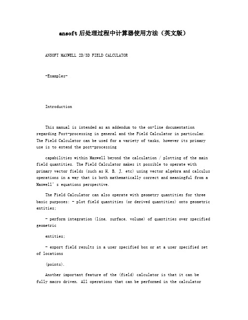
ansoft后处理过程中计算器使用方法(英文版)ANSOFT MAXWELL 2D/3D FIELD CALCULATOR-Examples-IntroductionThis manual is intended as an addendum to the on-line documentation regarding Post-processing in general and the Field Calculator in particular. The Field Calculator can be used for a variety of tasks, however its primary use is to extend the post-processingcapabilities within Maxwell beyond the calculation / plotting of the main field quantities. The Field Calculator makes it possible to operate with primary vector fields (such as H, B, J, etc) using vector algebra and calculus operations in a way that is both mathematically correct and meaningful from a Maxwell’s equations perspective.The Field Calculator can also operate with geometry quantities for three basic purposes: - plot field quantities (or derived quantities) onto geometric entities;- perform integration (line, surface, volume) of quantities over specified geometricentities;- export field results in a user specified box or at a user specified set of locations(points).Another important feature of the (field) calculator is that it can befully macro driven. All operations that can be performed in the calculatorhave a corresponding “image” in one or more lines of macro language code.Post-processing macros are widely used for repetitive post-processing operations, for support purposes and in cases whereOptimetrics is used and post-processing macros provide some quantityrequired in the optimization / parameterization process.This document describes the mechanics of the tools as well as the “softer” side of it as well. So, apart from describing the structure of the interfacethis document will show examples of how to use the calculator to perform manyof the post-processing operations encountered in practical, day to day engineering activity using Maxwell. Examples are grouped according to the typeof solution. Keep in mind that most of the examples can be easily transposedinto similar operations performed with solutions of different physical nature. Also most of the described examples have easy to find 2D versions.1. Description of the interfaceThe interface is shown in Fig. I1. It is structured such that it containsa stack which holds the quantity of interest in stack registers. A number of operations are intended to allow the user to manipulate the contents of thestack or change the order of quantities being hold in stack registers. The description of the functionality of the stack manipulation buttons (and of the corresponding stack commands) is presented below:- Push repeats the contents of the top stack register so that after the operation the twotop lines contain identical information;- Pop deletes the last entry from the stack (deletes the top of the stack);- RlDn (roll down) is a “circular” move that makes the co ntents of the stacks slidedown one line with the bottom of the stack advancing to the top;- RlUp (roll up) is a “circular” move that makes the contents of thestacks slide up oneline with the top of the stack dropping to the bottom;- Exch (exchange) produces an exchange between the contents of the two top stackregisters;- Clear clears the entire contents of all stack registers; - Undo reverses the result of the most recent operation.Stack & stack registersStackcommandsCalculator buttonsFig. I1 Field Calculator InterfaceThe user should note that Undo operations could be nested up to the level where a basic quantity is obtained.The calculator buttons are organized in five categories as follows:- Input contains calculator buttons that allow the user to enter data in the stack; sub-categories contain solution vector fields (B, H, J, etc.), geometry(point, line surface, volume), scalar, vector or complex constants (depending on application) or even entire f.e.m. solutions.- General contains general calculator operations that can be performed with “general”data (scalar, vector or complex), if the operation makes sense; for example if the top two entries on the stack are two vectors, one can perform the addition (+) but not multiplication (*);indeed, with vectors one can perform a dot product or a cross product but not a multiplication as it is possible with scalars.- Scalar contains operations that can be performed on scalars; example of scalars arescalar constants, scalar fields, mathematical operations performed on vector which result in a scalar, components of vector fields (such as the X component of a vector field), etc.- Vector contains operations that can be performed on vectors only; example of suchoperations are cross product (of two vectors), div, curl, etc.- Output contains operations resulting in plots (2D / 3D), graphs, data export, dataevaluation, etc.As a rule, calculator operations are allowed if they make sense from a mathematical point of view. There are situations however where the contents of the top stack registers should be in a certain order for the operation to produce the expected result. The examples that follow will indicate the steps to be followed in order to obtain the desired result in anumber of frequently encountered operations. The examples are grouped according to the type of solution (solver) used. They are typicalmedium/higher level post-processing task that can be encountered in current engineering practice. Throughout this manual it is assumed that the user has the basic skills of using the Field Calculator for basicoperations as explained in the on-line technical documentation and/or during Ansoft basic training.Note: The f.e.m. solution is always performed in the global (fixed) coordinate system. The plots of vector quantities are therefore related to the global coordinate system and will not change if a local coordinate system is defined with a different orientation from the global coordinate system.The same rule applies with the location of user defined geometry entities for post-processing purposes. For example the field value at a user-specified locati on (point) doesn’t change if the (local) coordinate system is moved around. The reason for this isthat the coordinates of the point are represented in the global coordinate system regardless of the current location of the local coordinate system.Electrostatic ExamplesExample ES1: Calculate the charge density distribution and total electric charge on the surface of an objectDescription: Assume an electrostatic (3D) application with separate metallic objects having applied voltages or floating voltages. The task is to calculate the total electric charge on any of the objects.a) Calculate/plot the charge density distribution on the object; the sequence of calculatoroperations is described below:- Qty -> D (load D vector into the calculator);- Geom -> Surface… (select the surface of interest) -> OK- Unit Vec -> Normal (creates the normal unit vector corresponding to the surface ofinterest)- Dot (creates the dot product between D and the unit normal vector to the surface ofinterest, equal to the surface charge density)- Geom -> Surface… (select the surface of interest) -> OK - Plotb) Calculate the total electric charge on the surface of an object- Qty -> D (load D vector into the calculator);- Geom -> Surface… (select the surface of interest) -> OK - Normal - ? - EvalExample ES2: Calculate the Maxwell stress distribution on the surface of an objectDescription: Assume an electrostatic application (for ex. a parallel plate capacitor structure). The surface of interest and adjacent region should have a fine finite element mesh since the Maxwell stress method for calculation the force is quite sensitive to mesh.The Maxwell electric stress vector has the following expression for objects without electrostrictive effects:感谢您的阅读,祝您生活愉快。

如何利用ansoft中磁路法计算,一键生成maxwell有限元电磁计算模型1、以一台凸极式永磁同步电机为例:打开软件,进入下图所示截面,选中RMxprt打开选择Adjust-Speed Synchronous Machine2、进入RMxprt界面,如下图所示:3、双击Machine,出现下图界面:极数:16转子位置:内转子各种损耗:可大致设置为额定功率的2%左右额定转速:790r/min线圈交流电AC及Y3星型联接4、双击stator,出现下图界面:定子外径:250定子内径:165定子轴向长度:160叠压系数:0.97定子材料:JFE_steel_50JN800定子槽数:36定子槽型:选3斜槽数:15、双击slot,如下图示:(一开始先将Auto Design后面√去除,点确认退出,再次双击slot 进入,即出现下图设置界面)3号槽型,设置数据如上图所示6、双击winding,选择winding界面线圈层数:2线圈形式:全极式绕组线圈并联之路:2每槽导体数:38(上下两层总计数)线圈跨距:4每匝线圈数:暂时空着,系统自动计算线圈漆包厚度:0.06平均线径:单击Diameter,进入设计截面,设置如下,点击OK再选择End/Insulation界面框线圈端部长:10槽绝缘厚度:0.3楔子厚度:2层绝缘厚:0.3槽满率:0.87、双击Rotor转子外径:162.5转子内径:110转子轴向长度:160转子材料:steel_1010叠压系数:1(转子为整个铸件)磁极类型:28、双击pole极狐系数:0.8偏移:0(即磁钢内外径同心)磁钢材料:NdFe35磁钢厚度:4.659、shaft轴可不设置10、右键单击Analysis单击选择Add solution setup,出现下图额定功率:17 (设置时注意单位的选择)额定电压:340额定转速:790其它默认即可11、至此RMxprt设置完成,右键点击增加的Setup1,单击Analyze 进行分析12、分析完成后可右键,可右键Results,选择Solution Data查看相关结果参数13、右键Setup1,选择Create Maxwell Design(生成有限元计算模型)选择Maxwell2D Design(或者3D,根据自己需求选择)14、系统会根据槽极比生成最小有限元单元,如此处生成1/4模型,若想生成全模型,可在RMxprt模块下,选择窗口中RMxprt,单击Design Settings,选择出现窗口下User Defined Date,设置如下(Fraction 1注意大小写及字母与数字间空一格),再点击重新计算即可生成有限元全模型谢谢!。
Ansoft Maxwell 2D/3D 使用说明第1章Ansoft 主界面控制面板简介在Windows下安装好Ansoft软件的电磁场计算模块Maxwell之后,点击Windows的“开始”、“程序”项中的Ansoft、Maxwell Control Panel,可出现主界面控制面板(如下图所示),各选项的功能介绍如下。
1.1 ANSOFT介绍Ansoft公司的联系方式,产品列表和发行商。
1.2 PROJECTS创建一个新的工程或调出已存在的工程。
要计算一个新问题或调出过去计算过的问题应点击此项。
点击后出现工程控制面板,可以实现以下操作:●新建工程。
●运行已存在工程。
●移动,复制,删除,压缩,重命名,恢复工程。
●新建,删除,改变工程所在目录。
1.3 TRANSLATORS进行文件类型转换。
点击后进入转换控制面板,可实现:1.将AutoCAD格式的文件转换成Maxwell格式。
2.转换不同版本的Maxwell文件。
1.4 PRINT打印按钮,可以对Maxwell的窗口屏幕进行打印操作。
1.5 UTILITIES常用工具。
包括颜色设置、函数计算、材料参数列表等。
第2章二维(2D)模型计算的操作步骤2.1 创建新工程选择Mexwell Control Panel (Mexwell SV)启动Ansoft软件→点击PROJECTS 打开工程界面(如图2.1所示)→点击New进入新建工程面板(如图2.2所示)。
在新建工程面板中为工程命名(Name),选择求解模块类型(如Maxwell 2D, Maxwell 3D, Maxwell SV等)。
Maxwell SV为Student Version即学生版,它仅能计算二维场。
在这里我们选择Maxwell SV version 9来完成二维问题的计算。
图2.1 工程操作界面图2.2 新建工程界面2.2 选择求解问题的类型上一步结束后,建立了新工程(或调出了原有的工程),进入执行面板(Executive Commands)如图2.3所示。
Ansoft Maxwell 2D/3D 使用说明目录第1章Ansoft 主界面控制面板简介第2章二维(2D)模型计算的操作步骤2.1 创建新工程 (2)2.2 选择求解问题的类型 (3)2.3 创建模型(Define Model) (4)2.4 设定模型材料属性(Setup Materials) (6)2.5 设定边界条件和激励源(Setup Boundaries/Sources) (8)2.6 设定求解参数(Setup Executive Parameters) (9)2.7 设定求解选项(Setup Solution Options) (10)2.8 求解(Solve) (10)2.9 后处理(Post Process) (11)2.10 工程应用实例 (12)第3章三维(3D)模型计算的操作步骤3.1 建模 (14)3.2 定义材料属性 (17)3.3 加载激励和边界条件 (18)3.4 设置求解选项和求解 (18)3.5 后处理 (18)3.6 补充说明 (18)3.7 例 1 两电极电场计算 (18)第4章有限元方法简介4.1 有限元法基本原理 (22)4.2 有限元网格自适应剖分方法 (23)第1章Ansoft 主界面控制面板简介在Windows下安装好Ansoft软件的电磁场计算模块Maxwell之后,点击Windows 的“开始”、“程序”项中的Ansoft、Maxwell Control Panel,可出现主界面控制面板(如下图所示),各选项的功能介绍如下。
1.1 ANSOFT介绍Ansoft公司的联系方式,产品列表和发行商。
1.2 PROJECTS创建一个新的工程或调出已存在的工程。
要计算一个新问题或调出过去计算过的问题应点击此项。
点击后出现工程控制面板,可以实现以下操作:●新建工程。
●运行已存在工程。
●移动,复制,删除,压缩,重命名,恢复工程。
●新建,删除,改变工程所在目录。
Ansoft Maxwell 2D/3D 使用说明(可参阅《Ansoft工程电磁场有限元分析》刘国强等编电子工业出版社)目录第1章Ansoft 主界面控制面板简介第2章二维(2D)模型计算的操作步骤2.1 创建新工程 (2)2.2 选择求解问题的类型 (3)2.3 创建模型(Define Model) (4)2.4 设定模型材料属性(Setup Materials) (6)2.5 设定边界条件和激励源(Setup Boundaries/Sources) (8)2.6 设定求解参数(Setup Executive Parameters) (9)2.7 设定求解选项(Setup Solution Options) (10)2.8 求解(Solve) (10)2.9 后处理(Post Process) (11)2.10 工程应用实例 (12)第3章三维(3D)模型计算的操作步骤3.1 建模 (14)3.2 定义材料属性 (17)3.3 加载激励和边界条件 (18)3.4 设置求解选项和求解 (18)3.5 后处理 (18)3.6 补充说明 (18)3.7 例 1 两电极电场计算 (18)第4章有限元方法简介4.1 有限元法基本原理 (22)4.2 有限元网格自适应剖分方法 (23)第1章Ansoft 主界面控制面板简介在Windows下安装好Ansoft软件的电磁场计算模块Maxwell之后,点击Windows 的“开始”、“程序”项中的Ansoft、Maxwell Control Panel,可出现主界面控制面板(如下图所示),各选项的功能介绍如下。
1.1 ANSOFT介绍Ansoft公司的联系方式,产品列表和发行商。
1.2 PROJECTS创建一个新的工程或调出已存在的工程。
要计算一个新问题或调出过去计算过的问题应点击此项。
点击后出现工程控制面板,可以实现以下操作:●新建工程。
●运行已存在工程。
●移动,复制,删除,压缩,重命名,恢复工程。
合成一个面如果操作过程中提示你操作会失去原来的面或者线的时候,不妨把面或者线先copy,操作了之后再paste就好。
Solid 用来生成体。
第一栏用来直接生成一些规则的体。
Sweep是通过旋转、拉伸面模型得到体。
第二栏是对体进行一些布尔操作,如加减等。
Split是将一个体沿一个面(xy、yz、xz)劈开成两部分,可以选择要保留的部分。
在减操作时,如有必要,还是先copy一下被减模型。
第三栏cover surface是通过闭合的曲面生成体。
Arrange 选取模型组件后,对模型组件进行移动、旋转、镜像(不保存原模型)、缩放等操作。
Options 用来进行一些基本的设置。
单位的转换,检查两个体是否有重叠(保存的时候会自动检查)、设置background大小、定义公式以及设置颜色。
二、材料设置相对比较简单,Maxwell材料库自带了一些常用的材料,如果没有可以自己新建一个材料。
Material—〉Add,输入文件名,及相关的参数即可。
如果BH曲线是非线性的,就,在B-H Nonlinear Material 前面打勾,就会有自己输入BH曲线的选项,自己输入就好。
但是要注意BH曲线是单调递增的。
新建的材料还可以设置为理想导体和各向异性的材料。
三、边界条件/激励的设置边界条件在3D模型中用的相对比较少,因为模型外层可以设置为真空区域,边界条件可以自动给出,如果是对称模型就可以设置相关的边界条件了。
我曾经做一个轴对称模型,相用模型的1/4计算,不过边界条件设置没有设对,可以自己摸索一下。
关于激励的设置,在加载电流的时候,最重要的一点是要将模型建立成一个回路。
否则的话无法得到正确的结果。
在回路中加电源的位置建一个截面,在截面上加载就好,注意截面要是平面,不能为曲面。
在进行瞬态分析的时候,Model—〉set eddy effect处设置有涡流效应的导体,处于有源回路上的导体不能设置涡流效应。
瞬态分析激励设置时,先将加载的面设置为Source :coil Terminal。
然后在Model—〉Winding Setup中设置。
一般是Function 里面,先定义一个Dataset,第一项为时间,第二项为对应的激励值。
然后用一个常量外推函数得到所要的值,格式为source_name=pwlx(T,constant,dataset_name).在设置激励的地方填上source_name就好。
四、求解量设置可以设置求解力、力矩、电感、Core loss的部件。
比如在设置求解力的时候可以先取一个组件名,然后选中该组件包含的导体。
力的求解选项中可以设置求解洛仑兹力和虚功力两种。
在一般条件下,两者的误差很小,但是在饱含铁区的模型中,用洛仑兹力求解会有很大的误差。
五、求解设置Option 里面设置一般的求解选项。
一般选用默认值就好了。
只是在进行瞬态分析的时候,建议先用同一个模型进行静态分析,然后将网格数据,所有以fileset1和fileset2命名的文件拷贝到瞬态分析的工程目录下面,将Starting Mesh设置成Current。
这时候进行瞬态分析的时候采用的就是静态分析时候的网格,求解精度比较高。
因为瞬态分析中,默认的网格仅进行一次简单的划分,而且没有能量误差的判断,所以求解的精度不能保证,但是这种设置有时候可能一次成功不了,可以多试几次,计算了一步,然后停下来,看看网格划分,如果是采用静态的网格划分,则继续,否则重新来。
后面两个选项是用来分析导体运动和参数化分析的选项。
六、后处理最简单的是Plot—〉field里面的相关选项了。
它可以划出磁场强度,磁感应强度,电流密度在各个部件的表面,体以及xy,yz,xy截面上的分布。
第一栏是选择要分析的量,mag H(B/J) 磁场强度,磁感应强度,电流密度的绝对值大小用来画云图的,H(B/J) Vector为它们的矢量,用来画矢量图。
后面几项没有用过,不知道具体干什么用的。
第二栏是画图所用的几何模型,比如surface xy就是在xy片面上话图。
Volume –all就是在所有的体上画图。
Animsurf xy则是在xy平面做动画。
注意,一些量不能在体上显示,如果选择体,会弹出警告。
第三栏是所显示的为哪个组件上的H(B/J)的值。
画出的云图和矢量图可以通过双击颜色标度栏,打开并设置一些显示参数,包括取值范围,颜色,箭头的大小和密度等,以大到最好的显示效果。
Plot—〉Visibility可以控制当前显示的内容。
Plot—〉Delete 删除已经建立出的后处理表达式。
还可以通过 Plot—〉save as将化出的云图保存为.dsp文件。
Plot—〉field的操作比较简单,但是它只能给出最基本的几个量,局限性比较大。
用Calculator 可以实现它里面所有的功能,而且可以扩展到其它的量的计算。
比如plot->field mag B,surface xy,-all-得到xy平面的磁场分布云图,在Calculator里面进行如下操作:Qty->B,Mag,Smooth,Geom->Volume->all,Domain,Geom->surface->xy,plot.即可实现该功能。
下面具体介绍一下Calculator中各个按钮的作用。
把显示区域当作一个堆栈来操作。
最上为栈顶,最下为栈底。
Push:将当前栈顶信息重行操作一遍,放在栈顶。
Pop:将栈顶操作出栈。
RlDn:将栈内的操作向下循环。
RlUp:将栈内的操作向上循环。
Exch:将栈顶的两条语句交换位置。
Clear:清空栈内的内容。
Undo:撤销操作。
Input:输入,获得一些基本的数据。
Qty:一些基本的计算结果,包括B、H、J、能量等;Geom:几何形状。
包括点、线、面、体。
这些元素一方面可以是前处理建模时候形成的,也可以根据需要,通过后处理器中的Geometry中相关选项创建。
Const:一些常数。
比如、,及一些单位转换时候所差的系数。
Num:输入的数字。
Func:一些公式。
Read:从之前保存的数据中读取,一般为.reg文件。
General:一般的操作,包括加减乘除、求反、求绝对值、平滑(smooth)、规定取数值的范围(Domain)。
Scalar:对标量的操作。
Vec? 将标量转化为矢量的x,y,z值。
其它的很容易理解,这是Iso我也不是很明白它是什么意思。
Vector:对矢量的操作。
Scal?将矢量的一个分量作为标量计算。
Matl… 将矢量乘或者除以一个电导率和磁导率。
Mag 取矢量的模。
Dot /Cross 点乘和叉乘Divg/Curl 散度和旋度Tangent 某一点的矢量值在切线方向上的投影Normal 某一点的矢量值面的法向上的投影。
Unit Vec?这个我也没有搞清楚Output 输出Draw 画出在后处理器中创建的几何模型Plot 画出calculator中存贮的在点线面体上的值。
首先求出你需要画图的值,比如洛仑兹力密度用F=BxJ,如果画云图然后smooth命令来改善一下显示的效果,再在Geom中选择要显示出计算值的几何模型。
然后Plot就好。
可以画出来的量有:1、面和体上的标量;2、面上的矢量;3、3维线上的标量和矢量;4、点上的标量和矢量。
Anim 动画制作,主要用在瞬态计算里面。
2D plot 一般用来画出一条线上的标量值。
横轴为先段上点到该线段起点的距离,纵轴为要求得值。
比如要知道电流沿导体厚度的分布规律时,可以沿导体厚度创建一条线,然后取得电流密度,2DPlot就可以画出电流密度随厚度的变化曲线。
Value 取得一系列的值,比如可以将上面例子中的点的坐标和对应的电流密度值对应起来,然后通过write命令写入到一个.reg文件中。
方便对数据进行其它的分析,例如和理论值比较等。
Eval 对直接能得出一个常量的公式求出其结果。
例如电流密度对一个面积分,就得到其电流。
现Qry-〉J,Geom-〉surface …,,eval。
就能得到结果。
Write 将结果写入文件。
Export 将数据导出,可以根据已经存有坐标的文件,到坐标相对应的值或者按栅格导出,即先将一个面划分成许多方形的小格子,导出格子每个顶点处对应的值。
首先选择你要导出的量,然后根据需要选择。
下面再举个例子,划出xy平面洛仑兹力的分布云图:Qty->B,Qty->J,cross,Mag,Smooth,Geom->Volume->all,Domain,Geom->surface->xy, plot注意:如果一个运算需要两个参数,那么先选出参数,然后再进行运算。
Plot的时候先计算出plot 的量,然后选择几何形状。
有时候操作顺序错了,系统会有警告,提示相关操作的顺序,另外建议大家还是先把帮助看明白在说。
Maxwell的前处理相对比较弱,但一般的模型都能够建立出。