fluent算例-船舶航行

fluent经典算例Tutorial:Modeling a Single-Channel,Counter-Flow Polymer Electrolyte Membrane(PEM)Fuel CellIntroductionThe purpose of this tutorial is to provide guidelines and recommendations for using the PEM Fuel Cell add-on module available in FLUENT.This tutorial demonstrates how to do the following:Build and generate a mesh for a single-channel PEM fuel cell.Assign zone names and types that are required in the FLUENT PEM fuel cell add-onmodule.Import the mesh into FLUENT,set up the case,and run the calculations.Postprocess the results.PrerequisitesThis tutorial assumes you are familiar with both the GAMBIT and FLUENT interfaces and that you have a good understanding of the basic setup and solution procedures.Details of most steps will not be shown explicitly.If you have not used FLUENT before,it would be helpful to?rst refer to the FLUENT6.3 User’s Guide and theFLUENT6.3Tutorial Guide.You can also refer to the GAMBIT User’s Guide,GAMBIT Tutorial Guide,and GAMBIT Modeling Guide.Problem DescriptionA schematic description of a single,straight-channel,counter-?ow PEM fuel cell is shown inFigure1.The dimensions of the fuel cell are2.4×2.88×125mm in the x,y,and z directions, respectively.This model represents a repeating channel of a larger counter-?ow PEM fuel cell.The cross-sectional area of the membrane electrode assemblyis2.4×125=300mm2.All the zones as marked in Figure1(with exception of the optional cooling channel)must be de?ned as separate zones within GAMBIT.Note that there can be multiples of each zone.For example,there can be multiple cathode gas di?usion layers,each with di?erent material properties.In FLUENT6.3,all continuum zones must be of the?uid type except for the current collectors which may be either solid or? uid.For simplicity,it is recommended that you make the current collectors solid continuum zones.Modeling a Single-Channel,Counter-Flow Polymer Electrolyte Membrane(PEM)Fuel CellFigure1:PEM Fuel Cell ZonesFor details about the FLUENT PEMFC model,refer to o f FLUENT6.3Fuel Cell ModulesManual.Note:If you would like to bypass all GAMBIT steps and proceed to the FLUENT portion of the tutorial,skip to Step. Preparation in GAMBIT1.Create a folder called pem-single-channel to contain the?les generated in thistutorial.2.Start GAMBIT and specify this folder as the working folder.To simplify the geometry construction and meshing steps,a journal?le,pem-single-channel.jou is provided.This?le contains GAMBIT instructions which will create the geometry and gen-erate the mesh.It is recommended that you step through the journal?le to understand eachof the steps and recognize the assigned zone boundary types pertinent to fuel cell problems.Geometry Creation and Mesh GenerationStep1:Geometry Creation1.Create a rectangular face primitive in the xy plane.Operation?→Geometry?→Face?→Create Real Rectangular Face(a)Enter2.4for Width and1.2for Height.Modeling a Single-Channel,Counter-Flow Polymer Electrolyte Membrane(PEM)Fuel Cell(b)Select+X+Y for Direction,(c)Click Apply and close the Create Real Rectangular Face panel.2.Create another face by sweeping the uppermost edge by0.21units in the y-direction.Operation?→Geometry?→Face?→Sweep Edges3.Create another face by sweeping the uppermost edge by0.012units in the y-direction.4.Create another face by sweeping the uppermost edge by0.036units in the y-direction.5.Create another face by sweeping the uppermost edge by0.012units in the y-direction.6.Create another face by sweeping the uppermost edge by0.21units in the y-direction.7.Create another face by sweeping the uppermost edge by1.2units in the y-direction.8.Create a rectangular face with dimensions(x,y)=(0.8,0.6).Use+x+y for the di-rection(so that the global coordinate system origin is in the lower left corner of theface).9.Move the newly created face using a vector of(0.8,0.6,0).Operation?→Geometry?→Face?→Move/Copy Faces10.Copy the face by1.08units in the y-direction.11.Split the lowermost face with the face you just created.Operation?→Geometry?→Face?→Split Face12.Similarly,split the uppermost face with its internal face.The resulting mesh should appear as shown in Figure2.Step2:Mesh Generation(Manual)1.Mesh the edges as shown in Figure2.The numbers of cells along each edge are indicated below.The geometry and mesh are symmetric about its horizontal midplane.Operation?→Mesh?→Edge?→Mesh Edges2.Mesh the nine faces using the Quad Submap scheme.Operation?→Mesh?→Face?→Mesh Faces3.Create an edge by sweeping any one of the vertices by125units in the positive z direction.Operation?→Geometry?→Edge?→Sweep VerticesModeling a Single-Channel,Counter-Flow Polymer Electrolyte Membrane(PEM)Fuel CellFigure2:Edge and Face Mesh(a)Select Vector for Path and click the De?ne button.(b)Enable Magnitude and enter125.(c)Select Positive for Z from the Direction list.(d)Click Apply in the Vector De?nition form.(e)Click Apply and close the Sweep Vertices form.4.Mesh the newly created edge using a double-sided graded edge mesh that consists of 60elements.(a)Enable Double sided.(b)Enter1.1for Ratio1and Ratio2.(c)Click Apply and close the Mesh Edges form.5.Create volumes by sweeping the nine faces along the newly created edge. Operation?→Geometry?→Volume?→Sweep Faces(a)Enable With Mesh.(b)Click Apply and close the Sweep Faces form.The volume mesh is as shown in Figure3.Modeling a Single-Channel,Counter-Flow Polymer Electrolyte Membrane(PEM)Fuel CellFigure3:Volume MeshStep3:Zone Assignments and Mesh ExportFLUENT’s PEM fuel cell add-on module requires that boundary and continuum zones berigorously de?ned.Care should be taken in order to have a logical system of naming eachzone to represent each of the regions shown in Figure1.At a minimum,the boundary zones that are required include the following:Inlet and outlet zones for the anode gas channel.Inlet and outlet zones for the cathode gas channel.Surfaces representing anode and cathode terminals.Optional boundary zones that could be de?ned include any voltage jump surfaces,interiorow surfaces,or non-conformal interfaces that are required.The following continuum zones are also required:Flow channels for anode-and cathode-sideuids.Anode and cathode current collectors.Anode and cathode gas diusion layers.Anode and cathode catalyst layers.Electrolyte membrane.The inlets should all be assigned the boundary zone type MASS FLOW INLET and outletsshould be assigned the PRESSURE OUTLET type.The terminals are the regions where thevoltage(or current?ux density)is known.Normally,the anode is grounded(V=0)andModeling a Single-Channel,Counter-Flow Polymer Electrolyte Membrane(PEM)Fuel Cell the cathode terminal is at a?xed potential that is less than the open-circuit potential.Bothof the terminals should be assigned the WALL boundary type.Voltage jump zones can optionally be placed between the various components(such asbetween the gas di?usion layer and the current collector).Faces which represent?uid/solidinterfaces must be of type WALL.Additional interior zones may be de?ned for purposes of post-processing.If such interiorzones are de?ned,they should have no e?ect on the solution.FLUENT’s PEM add-on module supports the use of non-conformal grid interfaces.In such cases,it is recommended that the INTERFACE boundary type be used halfway between the membrane continuum zone,and that the mesh on opposite sides of the interface have similar size,aspect ratio,and orientation.In such cases,the membrane will consist of two uid zones.1.Assign boundary zones according to the de?nitions listed in Table1.Operation?→Zones?→Specify Boundary TypesTable1:Boundary Zone AssignmentsAnode-side inlet(z=125,upper)inlet-a MASS FLOW INLETCathode-side inlet(z=0,lower)inlet-c MASS FLOW INLETAnode-side outlet(z=0,upper)outlet-a PRESSURE OUTLETCathode-side outlet(z=125,lower)outlet-c PRESSURE OUTLETAnode terminal(y=2.88)wall-terminal-a WALLCathode terminal(y=0)wall-terminal-c WALLAnode-side?ow channel walls wall-ch-a WALLCathode-side?ow channel walls wall-ch-c WALLFuel cell ends wall-ends WALLAnode-side di?usion layer walls wall-gdl-a WALLCathode-side di?usion layer boundaries wall-gdl-c WALLLateral boundaries of the fuel cell wall-sides WALL2.Assign continuum zones according to the de?nitions listed in Table2.Refer to Figure1 when selecting which volumes to assign to each zone.Operation?→Zones?→Specify Continuum TypesModeling a Single-Channel,Counter-Flow Polymer Electrolyte Membrane(PEM)Fuel Cell Table2:Continuum Zone AssignmentsAnode-side catalyst layer catalyst-a FLUIDCathode-side catalyst layer catalyst-c FLUIDAnode-side?ow channel channel-a FLUIDCathode-side?ow channel channel-c FLUIDAnode-side gas di?usion layer gdl-a FLUIDCathode-side gas di?usion layer gdl-c FLUIDElectrolyte membrane membrane FLUIDAnode current collector current-a SOLIDCathode current collector current-c SOLID3.Export the mesh?le as pem-single-channel.msh.Setup and Solution in FLUENTFLUENT’s PEM Fuel Cell(PEMFC)model is provided as an add-on module with thestandard FLUENT licensed software.A special license is required in order to use thismodel.The module is installed as part of the standard FLUENT installation in the folder/addons/fuelcells2.2within the FLUENT installation folder.The PEMFC model con-sists of a user-de?ned function(UDF)library and a compiled Scheme library which can beloaded using a text user interface(TUI)command.trtitlePreparation1.Copy the mesh?le pem-single-channel.msh.gz to your working folder.If you worked through the GAMBIT portion of this tutorial,an uncompressed versionof this?le will already be in place.2.Start the3DDP(3ddp)version of FLUENT.!If you wish to solve this case in parallel,you will need to set up and save the case?le in serial mode?rst.Once this is done,you can start a parallel FLUENTsession and proceed with the calculations.Step1:Grid1.Read the mesh?le,pem-single-channel.msh.gz.File?→Read?→Case...FLUENT will perform various checks on the mesh and will report the progress in theconsole window.Make sure that the reported minimum volume is a positive number.2.Check the grid.Grid?→CheckA grid check should always be performed in order to verify the integrity of the meshle.Specically,you should verify that the minimum cell volume is a positive value.Modeling a Single-Channel,Counter-Flow Polymer Electrolyte Membrane(PEM)Fuel Cell3.Since the mesh was created in units of millimeters,it must be scaled.Grid?→Scale...(a)Select mm from the Grid Was Created In drop-down list.(b)Click the Change Length Units button.(c)Click Scale.(d)Verify that the value of Zmax is125mm and close the Scale Grid panel.Step2:Models1.To load the PEMFC model using the text user interface,enter the following commandin the console:/define/models/addon-module3This command will load a Scheme library which contains the PEM model GUI anda UDF library.Upon successful execution,the following message will be displayed inthe console:Addon Module:fuelcells2.2...loaded!2.Calculate the surface area of the membrane for post-processing.In this case,the membrane area is equal to the surface area of the cathode terminal. This surface is named wall-terminal-c.Report?→Projected Areas...(a)Select Y from the Projection Direction group box.(b)Select wall-terminal-c from the Surfaces list.(c)Click Compute.The projected area reported is0.0003m2.(d)Close the Projected Surface Areas panel.3.Change the Solution Zones for user-de?ned scalars2and3to all zones.De?ne?→User-De?ned?→Scalars...This is an optional step which allows UDS-2and UDS-3to be postprocessed on bothuid and solid zones.4.Con?gure the PEM model.De?ne?→Models?→PEMFC...(a)Click the Anode tab.Modeling a Single-Channel,Counter-Flow Polymer Electrolyte Membrane(PEM)Fuel Cell i.Select Current Collector in the Anode Zone Type group box and select current-a from the Zone(s)selection list.ii.Select Flow Channel in the Anode Zone Type group box and select channel-afrom the Zone(s)selection list.iii.Select Di?usion Layer in the Anode Zone Type group box and select gdl-a fromthe Zone(s)selection list.iv.Select Catalyst Layer in the Anode Zone Type group box and select catalyst-afrom the Zone(s)selection list.(b)Click the Membrane tab.i.Select membrane from the Membrane Zone(s)selection list.(c)Click the Cathode tab.i.Select Current Collector in the Cathode Zone Type group box and selectcurrent-c from the Zone(s)selection list.ii.Select Flow Channel in the Cathode Zone Type and select channel-c from theZone(s)selection list.iii.Select Di?usion Layer in the Cathode Zone Type and select gdl-c from theZone(s)selection list.iv.Select Catalyst Layer in the Cathode Zone Type and select catalyst-c from theZone(s)selection list.(d)Click the Reports tab.i.Specify the value of Membrane-Electrode-Assembly Projected Area to0.0003m2. Recall that this value was obtained earlier in the tutorial.ii.Select wall-terminal-a from the Anode selection list and select wall-terminal-cfrom the Cathode selection list.(e)Click OK to close the PEM panel.FLUENT reports in the console that the energy equation has been enabled auto-matically.For convenience,the PEMFC model also automatically enables species transport and creates default materials.Step3:MaterialsRetain the default settings for the materials.Step4:Operating ConditionsDe?ne?→Operating Conditions...1.Set the Operating Pressure to200000pascal.2.Click OK to close the Operating Conditions panel.Modeling a Single-Channel,Counter-Flow Polymer Electrolyte Membrane(PEM)Fuel Cell Step5:Boundary ConditionsDe?ne?→Boundary Conditions...There are several zones which must be speci?ed in the boundary conditions panel.These are the anode and cathode voltage terminals,as well as the inlets and outlets.1.Set boundary conditions for the anode voltage terminal,wall-terminal-a.At this surface,the voltage is grounded and the temperature is constant.(a)Click the Thermal tab and enter353K for Temperature.(b)Click the UDS tab.i.Select Speci?ed Value from the Electric Potential drop-down list User-De?nedScalar Boundary Condition group box.ii.Enter0for Electric Potential in the User-De?ned Scalar Boundary Value groupbox.This boundary condition represents a grounded terminal.(c)Click OK to close the Wall panel.2.Set boundary conditions for the cathode voltage terminal,wall-terminal-c.At this surface,the voltage is maintained at a constant,positive value.(a)Click the Thermal tab and enter353K for Temperature.(b)Click the UDS tab.i.Select Speci?ed Value from the Electric Potential drop-down list User-De?nedScalar Boundary Condition group box.ii.Enter0.75for Electric Potential in the User-De?ned Scalar Boundary Valuegroup box.This boundary condition represents a terminal operating at0.75Volts.iii.Click OK to close the Wall panel.To calculate an IV polarization curve,you should vary the Electric Potential forthe cathode,starting from a voltage near the open circuit voltage and gradually decreasing it,converging the solution each time you change the value.3.Set boundary conditions for the anode gas?ow inlet,inlet-a.At this inlet,a humidi?ed hydrogen stream enters the fuel cell.No liquid enters the channel.(a)Enter6.0e-7kg/s for Mass Flow Rate and0for Supersonic/Initial Gauge Pressure.(b)Click the Thermal tab and enter353K for Temperature.(c)Click the Species tab and set the mass fractions of h2,o2and h2o to0.8,0.0,and0.2,respectively.(d)Click the UDS tab and select Speci?ed Value from the Water Saturation drop-down list in the User-De?ned Scalar Boundary Condition group box.Modeling a Single-Channel,Counter-Flow Polymer Electrolyte Membrane(PEM)Fuel Cell(e)Enter0for Water Saturation in the User-De?ned Scalar Boundary Value group box.(f)Click OK to close the Mass-Flow Inlet panel.4.Set boundary conditions for the cathode gas?ow inlet,inlet-c.At this inlet,a humidi?ed air stream enters the fuel cell.No liquid enters the channel.(a)Enter5.0e-6kg/s for Mass Flow Rate.(b)Click the Thermal tab and enter353K for Total Temperature.(c)Click the Species tab and set the mass fractions of h2,o2and h2o to0.0,0.2,and0.1,respectively.(d)Click the UDS tab and select Speci?ed Value from the Water Saturation drop-down list in the User De?ned Scalar Boundary Condition group box.(e)Enter0for Water Saturation in the User-De?ned Scalar Boundary Value group box.(f)Click OK to close the Mass-Flow Inlet panel.5.Set boundary conditions for the anode gas?ow outlet,outlet-a.(a)Click the Thermal tab and enter353K for Back?ow Total Temperature.(b)Click OK to close the Pressure Outlet panel.6.To set boundary conditions for the cathode gas?ow outlet,copy the boundary con-ditions from outlet-a to outlet-c7.Close the Boundary Conditions panel.Step6:Solution ControlsThe default solver settings are not su?cient to obtain a converged solution.Therefore,the following modi?cations must be made.1.Set the under-relaxation factor for Pressure to0.7,Momentum to0.3,Protonic Po-tential to0.95,and Water Content to0.95.Solve?→Controls?→Solution...2.Modify the multigrid settings.Solve?→Controls?→Multigrid...(a)Select F-Cycle from the Cycle Type drop-down lists for all equations.You will need to scroll down to set all equations.(b)Enter0.001for Termination Restriction for h2,o2,h2o,and Water Saturation.(c)Select BCGSTAB from the Stabilization Method drop-down list for h2,o2,h2o,Water Saturation,Electric Potential and Protonic Potential.(d)Enter0.0001for Termination Restriction for Electric Potential and Protonic Po-tential.(e)Increase the value of Max Cycles to50in the Algebraic Multigrid Controls group box.Modeling a Single-Channel,Counter-Flow Polymer Electrolyte Membrane(PEM)Fuel Cell(f)Click OK to close the Multigrid Controls panel.3.Enable the plotting of residuals.Solve?→Monitors?→Residual...Note:The PEMFC model automatically disables convergence checking for all equa-tions.4.Initialize the solution.Solve?→Initialize?→Initialize...(a)Set Temperature to353K.(b)Click Apply.(c)Click Init and close the Solution Initialization panel.5.Save the case and data?les as pem-single-channel.cas.gz andpem-single-channel.dat.gz.File?→Write?→Case&Data...!If you want to run the calculations in parallel,exit FLUENT and start a parallel session at this point.Open the case and data? les you saved in the previousstep and proceed.6.Request200iterations.The solution residuals will drop to acceptable values.Solve?→Iterate...The solution residual plot should resemble that shown in Figure4.The average currentdensity is displayed in the console at the end of each iteration.At the end of the calculations,the current density is reported as approximately0.324A/cm2.Step7:Postprocessing1.Create surfaces for postprocessing.Surface?→Iso-Surface...(a)Select Grid...and Z-Coordinate from the Surface of Constant drop-down lists.(b)Click Compute.(c)Enter62.5for Iso-Values(mm).(d)Enter plane-xy for New Surface Name.(e)Click Create.(f)Similarly,create another surface along the length of the fuel cell.This surfaceshould be a surface of constant X-Coordinate,with a value /doc/d88704d349649b6648d74700.html this surface plane-yz.(g)Close the Iso-Surface panel.Modeling a Single-Channel,Counter-Flow Polymer Electrolyte Membrane(PEM)Fuel CellFigure4:Residual Plot2.Create custom vectors for display.Display?→Vectors...(a)Click the Custom Vectors...button to open the Custom Vectors panel.i.Enter current-?ux-density for Vector Name.ii.Select User De?ned Memory...and X Current Flux Density from the X Com-ponent drop-down lists.iii.Select User De?ned Memory...and Y Current Flux Density from the Y Com-ponent drop-down lists.iv.Select User De?ned Memory...and Z Current Flux Density from the Z Com-ponent drop-down lists.v.Click De?ne and close the Custom Vectors panel.(b)Select current-?ux-density from the Vectors of drop-down list.(c)Select?lled-arrow from the Style drop-down list.(d)Click the Vector Options...button to open the Vector Options panel.i.Enter0.5for Scale Head.ii.Click Apply and close the Vector Options panel.(e)Select User-De?ned Memory and Current Flux Density Magnitude from the Colorby drop-down lists.(f)Enable Draw Grid from the Options list to open the Grid Display panel.i.Deselect all surfaces except plane-xy from the Surfaces selection list.Modeling a Single-Channel,Counter-Flow Polymer Electrolyte Membrane(PEM)Fuel CellFigure5:Current Flux at a Cross-Section Midway Down the Length of the PEM Channel ii.Ensure that Edges is enabled from the Options list and Feature is selectedfrom the Edge Type list.iii.Click Display and close the Grid Display panel.(g)Select plane-xy in the Surfaces selection list.(h)Click Display and close the Vectors panel.3.Auto-?t the display to the graphics window by pressing Ctrl-A on the keyboard./doc/d88704d349649b6648d74700.html pare your results with those shown in Figure5.Note:The maximum current density occurs in the regions between the channels and also that the plot units are A/m2.5.Plot contours of hydrogen mass fraction along the surface plane-yzDisplay?→Contours...(a)Enable Filled and Draw Grid from the Options list.(b)Select plane-yz from the Surfaces selection list in the Grid Display panel.(c)Click Display and close the Grid Display panel.(d)Restore the right view.Display?→View...i.Select right from the Views selection list.ii.Click Apply and close the Views panel.The display updates to the right-hand view.Modeling a Single-Channel,Counter-Flow Polymer Electrolyte Membrane(PEM)Fuel CellFigure6:Contours of Hydrogen Mass Fraction Along the Channel Length(e)Select plane-yz from the Surfaces selection list.(f)Select Species...and Mass fraction of h2from the Contours of drop-down lists.(g)Click Display.The resulting display is di?cult to visualize since the aspect ratio of the channelis large.You can change the way FLUENT displays data using the following steps:Display?→Scene...i.Select all entries from the Names selection list.ii.Click the Transform...button to open the Transformations panel.iii.Set Z to0.1in the Scale group box.iv.Click Apply and close the Transformations panel.The graphics display will be scaled accordingly.(h)Auto-?t the image to the window by pressing Ctrl-A in the graphics window.(i)Compare your result with that shown in Figure6.The?ow in the anode(upper)channel is from left to right.Note that the hydrogenmass fraction decreases in the direction of?ow.This is due to water being pulled through the membrane along with hydrogen as it is consumed in the fuel cell.6.Plot contours of oxygen mass fraction along the surface plane-yzDisplay?→Contours...(a)Follow the same procedure to generate the oxygen mass fraction contour plotthat you used to generate the hydrogen mass fraction contours.Modeling a Single-Channel,Counter-Flow Polymer Electrolyte Membrane(PEM)Fuel CellFigure7:Contours of Oxygen Mass Fraction Along the Channel Length(b)Compare your result with that shown in Figure7.The?ow in the cathode(lower) channel is from right to left.As expected,the oxygen mass fraction decreases inthe direction of?ow.7.Verify that global conservation of mass is observed.This will be done using a few text user interface(TUI)commands and basic electrochemistry concepts.(a)Compute the net oxygen consumption.Enter the TUI command:/report/species-mass-flowIf you have read a data?le instead of performing iterations,you must performat least one iteration in order to populate this data from the solver.The output is as follows:zone22(inlet-a):(4.8e-0701.2e-07)zone21(inlet-c):(01e-065e-07)zone20(outlet-a):(-4.6958153e-07-8.9805489e-11-2.8157297e-07)zone19(outlet-c):(-2.6251551e-10-9.1930928e-07-4.2904232e-07)zone53(wall-ch-a-shadow):(000)zone15(wall-ch-c):(000)zone29(wall-ends:029):(000)zone30(wall-ends:030):(000)zone31(wall-ends:031):(000)zone32(wall-ends:032):(000)zone33(wall-ends:033):(000)Modeling a Single-Channel,Counter-Flow Polymer Electrolyte Membrane(PEM)Fuel Cell zone51(wall-gdl-a-shadow):(000) zone11(wall-gdl-c):(000)zone1(wall-sides:001):(000)zone23(wall-sides:023):(000)zone25(wall-sides:025):(000)zone26(wall-sides:026):(000)zone27(wall-sides:027):(000)net species-mass-flow:(1.0155954e-088.0600915e-08-9.061529e-08)To interpret the output,each line can be read aszone num(zone-name):(˙m1˙m2...˙m n)where the subscripts1,2,...,nrefer to each species being calculated.Here,we are considering three species,namely h2,o2and h2o.Therefore,the second value in each list is the calculatedoxygen mass?ow rate in kilograms per second.In addition,a negative numberindicates?ow out of the domain from that boundary.From the last line,the netoxygen consumed is8.06×10?8kg/s.The molecular weight of oxygen is31.9988kg/kmol.Also,since the valence of a diatomic oxygen molecule is4,there are4kmol of electrons released per kmol of oxygen.Finally Faraday’s constant is9.6485×107C/kmol-electrons.Thus,the total release of electrons(which isequivalent to the current in Amperes),isI=˙mv FM=(8.06×10?8)(4.0)(9.6485×107)31.9988=0.972A(1)The total current is obtained by integrating the current density over the surface of the terminal.This integral value can be calculated in several ways.One way is to multiply the membrane area by the reported current density.This givesI=(0.0003)(0.3241)(100)2=0.972A(2) Alternatively,you can integrate the user memory Y Current Flux Density(the y-component of current density)over the terminal surface.This integration yields an accurate result since the y-direction is normal to the terminal.To do this, use the Surface Integrals panel.Report?→Surface Integrals...i.Select Report Type from the Integral drop-down list.ii.Select User De?ned Memory...and Y Current Flux Density from the Field Variable drop-down lists.iii.Select wall-terminal-a from the Surfaces selection list and click Compute.The absolute value of the number reported is approximately0.972A.We have electrochemical balance in the calculations. iv.Close the Surface Integrals panel.Modeling a Single-Channel,Counter-Flow Polymer Electrolyte Membrane(PEM)Fuel CellSummaryIn this tutorial,you learned how to set up and model a single-channel PEM fuel cell.Themodel provides detailed information on the distribution of current and voltage on all theelectrically conducting regions,along with species and current?ux density distributionthroughout the fuel cell.。

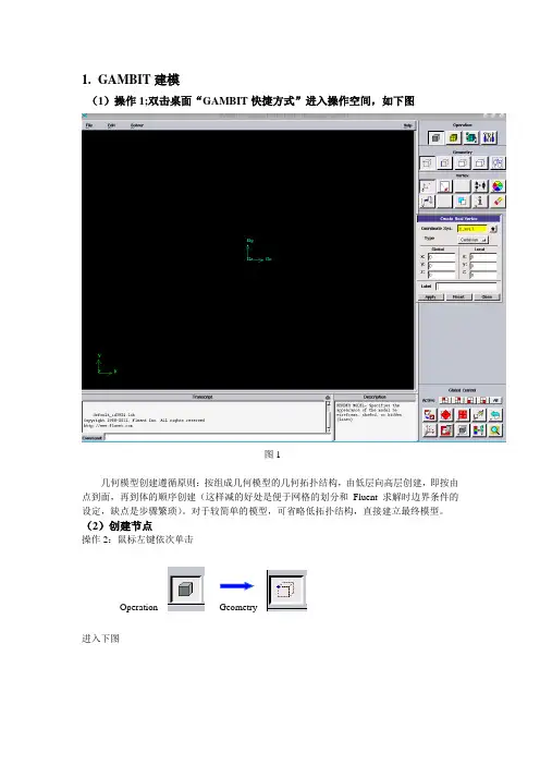
1.GAMBIT建模（1）操作1;双击桌面“GAMBIT快捷方式”进入操作空间，如下图图1几何模型创建遵循原则：按组成几何模型的几何拓扑结构，由低层向高层创建，即按由点到面，再到体的顺序创建（这样减的好处是便于网格的划分和Fluent求解时边界条件的设定，缺点是步骤繁琐）。

对于较简单的模型，可省略低拓扑结构，直接建立最终模型。

（2）创建节点操作2：鼠标左键依次单击Operation Geometry进入下图图2操作3：左键单击上图Apply，创建第一个点（坐标（0、0、0）），如下图，可以发现坐标原点显示白色图3操作4：在上图2中Global下输入x：200，y：0，z: 0，左键单击Apply, 如下图，操作5：左键单击（作用：窗口显示），如下图重复操作4和操作5，以此建立点（0，-0.0025,0）、（0.05，-0.0025，0）、（0.05、-0.0125）（0.15,0.0025,0），（0.15,0.0125，0），（0.2,0.0025），如下图，（3）节点成线操作1：左键依次单击，然后Shift+鼠标左键依次（为沿围成图形各点顺序）单击所创建的点，如下图，左键单击Apply，如下图，（4）连线成面操作1：左键单击，Shift+左键依次单击图中各线段，如下图，左键单击Apply，如下图，（5）网格划分网格划分遵循原则与模型创建类似操作1：左键依次单击，如下图，操作2：Shift+左键选中模型中一条边操作3：左键单击，弹出菜单中选择interval count，在左侧输入框中输入;200(为该条边上网格节点数)，如下图重复操作2和操作3，将沿y方向的短边和长边节点数分别设定为20和80.注意：对于相互平行两边，节点设置可只在一边进行；如果两边均设定，切记两边节点数要一致。

操作4：左键单击，Shift+左键单击图中任一边，所有边显示红色，然后左键单击Apply，如下图，（6）设置边界类型操作1: 左键单击，如下图，操作2：Shift+左键单击模型最左侧沿y方向的短边（显红色），单击，弹出菜单中选择PRESSURE-INLET，左键单击Apply，如下图，操作3：Shift+左键单击模型最右侧沿y方向的短边（显红色），单击，弹出菜单中选择PRESSURE-OUTLET，左键单击Apply，如下图，操作4：其它边不设置，默认为壁面条件。

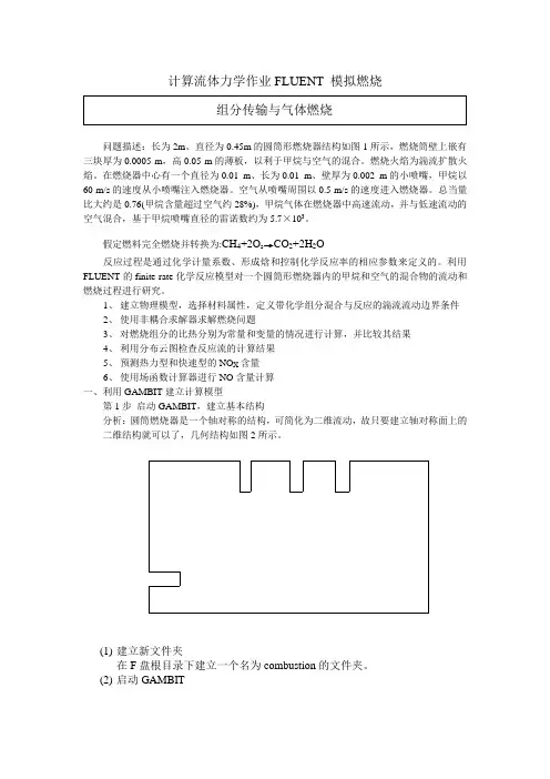
计算流体力学作业FLUENT 模拟燃烧问题描述：长为2m、直径为0.45m的圆筒形燃烧器结构如图1所示，燃烧筒壁上嵌有三块厚为0.0005 m，高0.05 m的薄板，以利于甲烷与空气的混合。

燃烧火焰为湍流扩散火焰。

在燃烧器中心有一个直径为0.01 m、长为0.01 m、壁厚为0.002 m的小喷嘴，甲烷以60 m/s的速度从小喷嘴注入燃烧器。

空气从喷嘴周围以0.5 m/s的速度进入燃烧器。

总当量比大约是0.76(甲烷含量超过空气约28%)，甲烷气体在燃烧器中高速流动，并与低速流动的空气混合，基于甲烷喷嘴直径的雷诺数约为5.7×103。

假定燃料完全燃烧并转换为:CH4+2O2→CO2+2H2O反应过程是通过化学计量系数、形成焓和控制化学反应率的相应参数来定义的。

利用FLUENT的finite-rate化学反应模型对一个圆筒形燃烧器内的甲烷和空气的混合物的流动和燃烧过程进行研究。

1、建立物理模型，选择材料属性，定义带化学组分混合与反应的湍流流动边界条件2、使用非耦合求解器求解燃烧问题3、对燃烧组分的比热分别为常量和变量的情况进行计算，并比较其结果4、利用分布云图检查反应流的计算结果5、预测热力型和快速型的NO X含量6、使用场函数计算器进行NO含量计算一、利用GAMBIT建立计算模型第1步启动GAMBIT，建立基本结构分析：圆筒燃烧器是一个轴对称的结构，可简化为二维流动，故只要建立轴对称面上的二维结构就可以了，几何结构如图2所示。

(1)建立新文件夹在F盘根目录下建立一个名为combustion的文件夹。

(2)启动GAMBIT(3)创建对称轴①创建两端点。

A(0,0,0)，B(2,0,0)②将两端点连成线(4)创建小喷嘴及空气进口边界②连接AC、CD、DE、DF、FG。

(5)创建燃烧筒壁面、隔板和出口②将H、I、J、K、L、M、N向Y轴负方向复制，距离为板高度0.05。

③连接GH、HO、OP、PI、IJ、JQ、QR、RK、KL、LS、ST、TM、MN、NB。

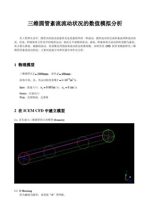
三维圆管紊流流动状况的数值模拟分析在工程和生活中，圆管内的流动是最常见也是最简单的一种流动，圆管流动有层流和紊流两种流动状况。

层流，即液体质点作有序的线状运动，彼此互不混掺的流动；紊流，即液体质点流动的轨迹极为紊乱，质点相互掺混、碰撞的流动。

雷诺数是判别流体流动状态的准则数。

本研究用CFD 软件来模拟研究三维圆管的紊流流动状况，主要对流速分布和压强分布作出分析。

1 物理模型三维圆管长2000mm l =，直径100mm d =。

流体介质：水，其运动粘度系数62110m /s ν-=⨯。

Inlet ：流速入口，10.005m /s υ=，20.1m /s υ= Outlet ：压强出口Wall ：光滑壁面，无滑移2 在ICEM CFD 中建立模型2.1 首先建立三维圆管的几何模型Geometry2.2 做Blocking因为截面为圆形，故需做“O ”型网格。

2.3 划分网格mesh注意检查网格质量。

在未加密的情况下，网格质量不是很好，如下图因管流存在边界层，故需对边界进行加密，网格质量有所提升，如下图2.4 生成非结构化网格，输出fluent.msh 等相关文件3 数值模拟原理紊流流动当以水流以流速20.1m /s υ=，从Inlet 方向流入圆管，可计算出雷诺数10000υdRe ν==，故圆管内流动为紊流。

假设水的粘性为常数（运动粘度系数62110m /s ν-=⨯）、不可压流体，圆管光滑，则流动的控制方程如下：①质量守恒方程：()()()0u v w t x y zρρρρ∂∂∂∂+++=∂∂∂∂ (0-1)②动量守恒方程：2()()()()()()()()()()[]u uu uv uw u u ut x y z x x y y z z u u v u w p x y z xρρρρμμμρρρ∂∂∂∂∂∂∂∂∂∂+++=++∂∂∂∂∂∂∂∂∂∂'''''∂∂∂∂+----∂∂∂∂ (0-2)2()()()()()()()()()()[]v vu vv vw v v v t x y z x x y y z z u v v v w px y z yρρρρμμμρρρ∂∂∂∂∂∂∂∂∂∂+++=++∂∂∂∂∂∂∂∂∂∂'''''∂∂∂∂+----∂∂∂∂ (0-3)2()()()()()()()()()()[]w wu wv ww w w w t x y z x x y y z z u w v w w px y z zρρρρμμμρρρ∂∂∂∂∂∂∂∂∂∂+++=++∂∂∂∂∂∂∂∂∂∂'''''∂∂∂∂+----∂∂∂∂ (0-4)③湍动能方程：()()()()[())][())][())]t t k k t k k k ku kv kw k k t x y z x x y yk G z zμμρρρρμμσσμμρεσ∂∂∂∂∂∂∂∂+++=+++∂∂∂∂∂∂∂∂∂∂+++-∂∂ (0-5)④湍能耗散率方程：212()()()()[())][())][())]t t k k t k k u v w t x y z x x y y C G C z z k kεεμμρερερερεεεμμσσμεεεμρσ∂∂∂∂∂∂∂∂+++=+++∂∂∂∂∂∂∂∂∂∂+++-∂∂ (0-6)式中，ρ为密度，u 、ν、w 是流速矢量在x 、y 和z 方向的分量，p 为流体微元体上的压强。

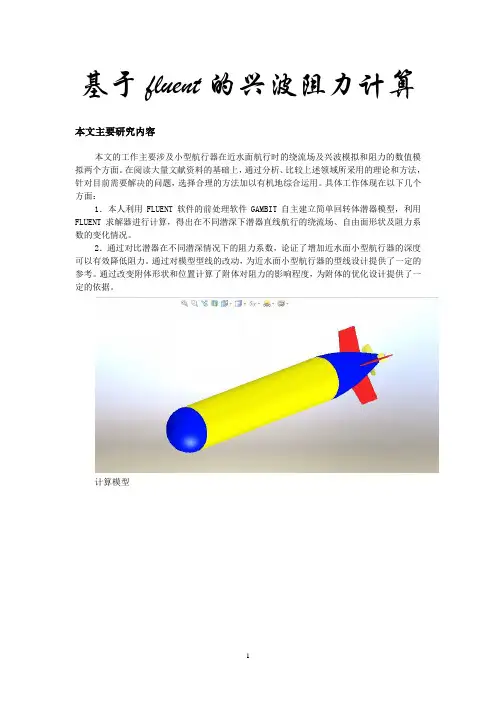
基于fluent的兴波阻力计算本文主要研究内容本文的工作主要涉及小型航行器在近水面航行时的绕流场及兴波模拟和阻力的数值模拟两个方面。

在阅读大量文献资料的基础上，通过分析、比较上述领域所采用的理论和方法，针对目前需要解决的问题，选择合理的方法加以有机地综合运用。

具体工作体现在以下几个方面：1．本人利用FLUENT软件的前处理软件GAMBIT自主建立简单回转体潜器模型，利用FLUENT求解器进行计算，得出在不同潜深下潜器直线航行的绕流场、自由面形状及阻力系数的变化情况。

2．通过对比潜器在不同潜深情况下的阻力系数，论证了增加近水面小型航行器的深度可以有效降低阻力。

通过对模型型线的改动，为近水面小型航行器的型线设计提供了一定的参考。

通过改变附体形状和位置计算了附体对阻力的影响程度，为附体的优化设计提供了一定的依据。

计算模型航行器粘性流场的数值计算理论水动力计算数学模型的建立根据流体运动时所遵循的物理定律，基于合理假设（连续介质假设）用定量的数学关系式表达其运动规律，这些表达式成为流体运动的数学模型，它们是对流体运动的一种定量模型化，称为流体运动控制方程组。

根据控制方程组，结合预先给定的初始条件和边界条件，就可以求解反映流体运动的变量值，从而实现对流体运动的数值模拟预报，形成分析报告。

基于连续介质假设的流体力学中流体运动必须满足要遵循的物理定律:1) 质量守恒定律2）动量守恒定律3）能量守恒定律4）组分质量守恒方程针对具体研究的问题，有选择的满足上述四个定律。

船体的粘性不可压缩绕流运动，如果不考虑水温对水物理性质的影响，水的密度和分子粘性系数都是常数，同时没有能量的转换，就仅仅需要满足质量守恒定律、动量守恒定律。

在满足这些定律下所建立的数学模型称为Navier-Stokes方程。

另外，自由液面的存在也需要建立合适的数学模型。

本文是利用FLUENT 进行数值模拟，而软件里面关于自由液面模拟是用界面追踪方法的一种－流体体积法（VOF）,基于该方法所建立的数学模型称为流体体积分数方程。

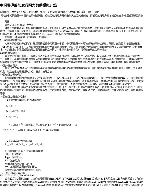
中间渠道船舶航行阻力数值模拟计算发布时间：2023-02-21T01:09:22.765Z 来源：《工程建设标准化》2022年19期10月作者：冯伟[导读] 中间渠道是一种特殊的限制性航道，船舶的航行阻力是确定其尺度的关键参数，而船舶航行阻力又与船舶航速,中间渠道的断面系数冯伟重庆交通大学重庆 400074摘要：中间渠道是一种特殊的限制性航道，船舶的航行阻力是确定其尺度的关键参数，而船舶航行阻力又与船舶航速,中间渠道的断面系数，下沉量有着一定的关系，本文采用数值模拟的方法，采用flow3d，测定了3000吨级单散货船在不同断面系数（1-5），不同航速下的船舶阻力值，通过对数值模拟结果进行分析，总结出船舶航行阻力变化的趋势关键字：中间渠道；数值模拟；船舶阻力1．中间渠道研究现状对于梯级船闸和升船机间，通常需要设置中间渠道来串联，中间渠道是一种两端封闭的限制性航道，然而，在我国《内河通航标准（GB 50139—2014）》中，对限制性航道和船闸尺度等均有规定，但对中间渠道这种特殊限制性渠道的断面尺度，尚未制定专门的通航标准。

本文通过对中间渠道船舶阻力进行数值模拟计算，以求探索出一种有关中间渠道的尺度的设计规范。

1.1国内研究现状关于中间渠道的研究，一方面，前人多以研究中间渠道内非恒定流水流特性，通航水流，以及渠道尺度与渠道内船舶航行方式等为主。

周华兴，高学平利用物理模型结合数学模型, 研究船闸泄水进入中间渠道后, 中间渠道内的水流条件与渠道尺度的关系。

根据波动特性,对渠道内水体波动进行了定义。

试验发现, 船闸泄水正波在前进中波前逐渐变陡, 到一定程度, 波前水体形状将不再稳定, 并形成短周期波。

1.2国外研究现状美国1953 年对 Welland 运河和船闸中间渠道的涌浪问题进行了原体观测和室内试验，提出减轻涌浪可采用降低灌泄水速度，加大河道尺度，制定合理的船闸运转方式、设调节池等方法1.3船舶阻力研究现状船舶阻力即是指的是船舶在航行中受到的阻力，一般分为三部分，一部分为兴波阻力Rw，一部分为船体摩擦阻力Rg ，一部分为黏剩余阻力Rvp，各种阻力成分在总阻力中所占比重在不同航速的船中是不相同的，对于低速船来说，摩擦阻力Rf占总阻力的70%-80%，黏剩余阻力Rvp约等于或大于10%，而兴波阻力Rw成分很小；对于高速船，Rf约占总阻力的40%-50%，而兴波阻力Rw却可达50%左右。

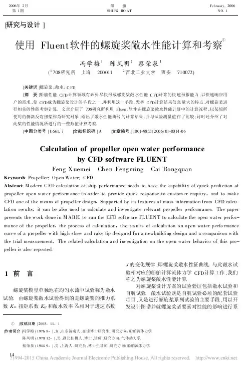
[研究与设计]使用Fluent 软件的螺旋桨敞水性能计算和考察①冯学梅1　陈凤明2　蔡荣泉1(1708研究所　上海　200011 2西北工业大学　西安　710072) [关键词]螺旋桨;敞水;C FD[摘　要]船舶性能CFD 计算领域有必要尽快形成螺旋桨敞水性能C FD 计算的快速预报能力,以快速响应用户的需求,使CFD 成为螺旋桨设计的手段之一,并利用这一手段,发挥CFD 计算结果信息量大的特点,对螺旋桨进行相关的性能考察计算。

文章介绍了708研究所利用Fluent 软件在螺旋桨敞水性能计算中的计算流程,以某船所使用的侧斜反弯扭桨作为研究对象,给出了敞水性能曲线的计算结果,并与试验测量值作了比较;同时还介绍了对此桨的性能情况所进行的一些数值计算考察。

[中图分类号]U661.7 [文献标识码]A [文章编号]1001-9855(2006)01-0014-06Calculation of propeller open water performanceby CFD software FLUENTFeng X uemei Chen Feng ming Cai Rong quanKeywords :Pro peller;Open Wa ter;CFDAbstract :M odern C FD calculation o f ship perfo rmance needs to hav e the capability of quick prediction of propeller open w ater perfo rm ance in o rder to prov ide quick response to custom er enquiry ,and to makeCFD one of the mea ns of propeller desig n .Suppo rted by its fea tures o f mass info rmatio n from CFD calcu-lation results,it can be also used to calculate a nd inv estigate releva nt pro peller perfo rm ance.The paper presents the w ork done in M ARIC to run the CFD softw are FLUEN T to calculate the open w ater perfo r-ma nce o f the pro peller ,the process of calcula tion ,the results of calcula tion o n o pen wa ter perfo rmance curv e of a pro peller w ith hig h skew a nd rake tip designed fo r a newbuilding design and a co mpa rison w ith the trial m easurement.The related calculation a nd inv estiga tion on the open w ater behavio r of this pro-peller is also repo rted .1　前　言螺旋桨模型单独地在均匀水流中试验称为敞水试验。

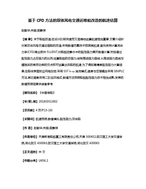
基于CFD方法的双体风电交通运维船改造的航速估算赵敏华;关超;吴静萍【摘要】关于船舶改造,在设计阶段快速而又准确地估算航速相当重要.文章介绍针对某双体风电交通运维船的改造,采用数值仿真技术预报其航速.首先使用计算流体力学(CFD)商业软件FLUENT,对船舶在静水中的黏性阻力展开数值计算.然后通过黏性阻力占总阻力的比例,估算船舶的总阻力,绘制推进阻力曲线.从推进阻力曲线与螺旋桨的有效功率的交点即可估算出该船的航速.为了得到高精度黏性阻力计算结果,在船体表面附近网格加密,采用SST k-ω湍流模式,速度与压强耦合采用SIMPLC 方法,其它离散采用二阶迎风格式.数值方法预报船舶黏性阻力技术相当成熟,发表的数值预报结果供读者参考.【期刊名称】《中国修船》【年(卷),期】2018(031)002【总页数】4页(P13-16)【关键词】航速预报;数值模拟;黏性阻力;双体船【作者】赵敏华;关超;吴静萍【作者单位】天津新港船舶重工有限责任公司,天津300452;武汉理工大学交通学院,湖北武汉430063;武汉理工大学交通学院,湖北武汉430063【正文语种】中文【中图分类】U656.2关于船舶改造，在设计阶段快速而又准确地估算航速相当重要。

航速估算可以通过不同航速下阻力估算得到船舶的推进阻力曲线;然后根据主机功率和螺旋桨推进系数计算螺旋桨的有效功率，从而由推进阻力曲线和有效功率估算出航速［1］。

螺旋桨的有效功率通过估算船厂提供的主机功率或螺旋桨收到效率，考虑螺旋桨敞水效率、船身效率的影响，参考教材提供的数据［1］，估计1个敞水效率和船身效率，最后得到有效功率。

船舶主机功率确定之后，螺旋桨的有效功率比较容易估算，关键问题在于船舶的总阻力的估算。

船舶在波浪中航行，阻力主要包括黏性阻力、兴波阻力、空气阻力和波浪增阻4大部分。

对于中低速排水量型船舶，其中黏性阻力是主要部分，其它阻力成份，如兴波阻力、空气阻力和波浪增阻，各占一定比例［2］。

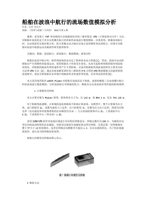
船舶在波浪中航行的流场数值模拟分析作者：汪异周文平来源：《发明与创新·大科技》 2018年第1期摘要：采用基于VOF和高精度自由面捕捉技术的三维非稳态CFD（计算流体动力学）方法，对船舶在迎浪状态下多自由度耦合航行时的粘性流场进行数值模拟。

结果表明：船舶迎浪航行时，自由面波形呈现对称分布，阻力系数及动力响应呈现正弦周期性变化的特点。

结果可为船舶在波浪中摇荡运动及耐波性研究提供指导。

关键词：船舶；迎浪航行；斜浪航行；数值模拟；流场分析船舶在波浪中航行时，粘性绕流场状态决定了船体的水动力性能[1]。

然而，波浪中运动的船舶会产生周期性的摇荡运动，使得船舶水下形状发生变化，从而引起船体周围的粘性绕流场的变化，对船舶的耐波性和快速性等产生不利影响。

目前对船舶粘性绕流场的研究主要有实验方法和CFD方法 [2]。

通过直接求解雷诺时均三维粘性N-S方程的CFD数值模拟方法能得到绕流场细节，进而分析船舶在水环境中的耐波性及快速性等性能，具有明显的优势[3]。

本文采用商用软件ANSYS Fluent对船舶在迎浪状态下纵摇、垂荡和横摇三自由度耦合航行时的流场进行数值模拟，分析迎浪航行对船舶的阻力、横摇及自由表面波形等性能的影响规律。

1.计算模型及网格本文计算对象为Wigley船型，船体基本尺寸为：长L=2 m，宽B=0.2 m，吃水T=0.125 m。

对于船舶绕流建模，计算域的选取要确保不影响计算流场。

本模型中，整个计算域为长方体，进口距船首2L，设置为速度入口边界；出口距船尾4L，设置为压力出口边界；四面为对称边界（法向速度和其他物理量的法向梯度均为0）：左右表面距船体中心2L，上表面距中心0.2L，下表面距中心（即水深）1.5L。

采用ICEM-CFD软件对流场区域进行非结构化网格划分，网格总数约为250万。

为确保对边界层内的流动特性的良好捕捉，对船身近壁面生成棱柱体边界层网格，且保证第一层网格被布置于Y+小于10的范围内、边界层网格法向膨胀率不超过1.2。

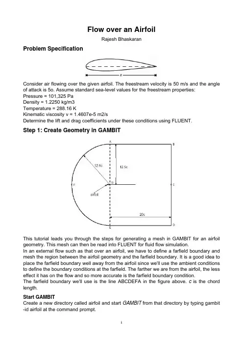
Flow over an AirfoilRajesh BhaskaranProblem SpecificationConsider air flowing over the given airfoil. The freestream velocity is 50 m/s and the angle of attack is 5o. Assume standard sea-level values for the freestream properties:Pressure = 101,325 PaDensity = 1.2250 kg/m3Temperature = 288.16 KKinematic viscosity v = 1.4607e-5 m2/sDetermine the lift and drag coefficients under these conditions using FLUENT.Step 1: Create Geometry in GAMBITThis tutorial leads you through the steps for generating a mesh in GAMBIT for an airfoil geometry. This mesh can then be read into FLUENT for fluid flow simulation.In an external flow such as that over an airfoil, we have to define a farfield boundary and mesh the region between the airfoil geometry and the farfield boundary. It is a good idea to place the farfield boundary well away from the airfoil since we'll use the ambient conditions to define the boundary conditions at the farfield. The farther we are from the airfoil, the less effect it has on the flow and so more accurate is the farfield boundary condition.The farfield boundary we'll use is the line ABCDEFA in the figure above. c is the chord length.Start GAMBITCreate a new directory called airfoil and start GAMBIT from that directory by typing gambit -id airfoil at the command prompt.Under Main Menu, select Solver > FLUENT 5/6 since the mesh to be created is to be used in FLUENT 6.0.Import EdgeTo specify the airfoil geometry, we'll import a file containing a list of vertices along the surface and have GAMBIT join these vertices to create two edges, corresponding to the upper and lower surfaces of the airfoil. We'll then split these edges into 4 distinct edges to help us control the mesh size at the surface.Let's take a look at the vertices.dat file:The first line of the file represents the number of points on each edge (61) and the number of edges (2). The first 61 set of vertices are connected to form the edge corresponding to the upper surface; the next 61 are connected to form the edge for the lower surface.The chord length c for the geometry in vertices.dat file is 1, so x varies between 0 and 1. If you are using a different airfoil geometry specification file, note the range of x values in the file and determine the chord length c. You'll need this later on.Main Menu > File > Import > ICEM Input ...For File Name, browse and select the vertices.dat file. Select both Vertices and Edges under Geometry to Create: since these are the geometric entities we need to create. Deselect Face. Click Accept.Split EdgesNext, we will split the top and bottom edges into two edges each as shown in the figure below.We need to do this because a non-uniform grid spacing will be used for x<0.3c and a uniform grid spacing for x>0.3c. To split the top edge into HI and IG, selectMake sure Point is selected next to Split With in the Split Edge window.Select the top edge of the airfoil by Shift-clicking on it. You should see something similar to the picture below:We'll use the point at x=0.3c on the upper surface to split this edge into HI and IG. To do this, enter 0.3 for x: under Global. If your c is not equal to one, enter the value of 0.3*c instead of just 0.3.For instance, if c=4, enter 1.2. From here on, whenever you're asked to enter (some factor)*c, calculate the appropriate value for your c and enter it.You should see that the white circle has moved to the correct location on the edge.Click Apply. You will see a message saying ``Edge edge.1 was split, and edge edge.3 created'' in the Transcript window.Note the yellow marker in place of the white circle, indicating the original edge has been split into two edges with the yellow marker as its dividing point.Repeat this procedure for the lower surface to split it into HJ and JG. Use the point at x=0.3c on the lower surface to split this edge.Create Farfield BoundaryNext we'll create the farfield boundary by creating vertices and joining them appropriately to form edges.Create the following vertices by entering the coordinates under Global and the label under Label:Click the FIT TO WINDOW button to scale the display so that you can see all the vertices.As you create the edges for the farfield boundary, keep the picture of the farfield nomenclature given at the top of this step handy.Create the edge AB by selecting the vertex A followed by vertex B. Enter AB for Label. Click Apply. GAMBIT will create the edge. You will see a message saying something like "Created edge: AB'' in the Transcript window.Similarly, create the edges BC, CD, DE, EG, GA and CG. Note that you might have to zoom in on the airfoil to select vertex G correctly.Next we'll create the circular arc AF. Right-click on the Create Edge button and select Arc.In the Create Real Circular Arc men o Center will be yellow. That meansu, the box next tthat the vertex you select will be taken as the center of the arc. Select vertex G and click Apply.Now the box next to End Points will be highlighted in yellow. This means that you can now select the two vertices that form the end points of the arc. Select vertex A and then vertex F. Enter AF under Label. Click Apply.If you did this right, the arc AF will be created. If you look in the transcript window, you'll see a message saying that an edge has been created.Similarly, create an edge corresponding to arc EF.Create FacesThe edges can be joined together to form faces (which are planar surfaces in 2D). We'll create three faces: ABCGA, EDCGE and GAFEG+airfoil surface. Then we'll mesh each face.This brings up the Create Face From Wireframe menu. Recall that we had selected vertices in order to create edges. Similarly, we will select edges in order to form a face.To create the face ABCGA, select the edges AB, BC, CG, and GA and click Apply. GAMBIT will tell you that it has "Created face: face.1'' in the transcript window.Similarly, create the face EDCGE.To create the face consisting of GAFEG+airfoil surface, select the edges in the following order: AG, AF, EF, EG, and JG, HJ, HI and IG (around the airfoil in the clockwise direction). Click Apply.Step 2: Mesh Geometry in GAMBITMesh FacesWe'll mesh each of the 3 faces separately to get our final mesh. Before we mesh a face, we need to define the point distribution for each of the edges that form the face i.e. we first have to mesh the edges. We'll select the mesh stretching parameters and number of divisions for each edge based on three criteria:1.We'd like to cluster points near the airfoil since this is where the flow is modified the most; the meshresolution as we approach the farfield boundaries can become progressively coarser since the flow gradients approach zero.2.Close to the surface, we need the most resolution near the leading and trailing edges since these arecritical areas with the steepest gradients.3.We want transitions in mesh size to be smooth; large, discontinuous changes in the mesh sizesignificantly decrease the numerical accuracy.The edge mesh parameters we'll use for controlling the stretching are successive ratio, first length and last length. Each edge has a direction as indicated by the arrow in the graphics window. The successive ratio R is the ratio of the length of any two successive divisions in the arrow direction as shown below. Go to the index of the GAMBIT User Guide and look under Edge>Meshing for this figure and accompanying explanation. This help page also explains what the first and last lengths are; make sure you understand what they are.Select the edge GA. The edge will change color and an arrow and several circles will appear on the edge. This indicates that you are ready to mesh this edge. Make sure the arrow is pointing upwards. You can reverse the direction of the edge by clicking on the Reverse button in the Mesh Edges menu. Enter a ratio of 1.15. This means that each successive mesh division will be 1.15 times bigger in the direction of the arrow. Select Interval Count under Spacing. Enter 45 for Interval Count. Click Apply. GAMBIT will create 45 intervals on this edge with a successive ratio of 1.15.For edges AB and CG, we'll set the First Length (i.e. the length of the division at the start of the edge) rather than the Successive Ratio. Repeat the same steps for edges BC, AB and CG with the following specifications:Note that later we'll select the length at the trailing edge to be 0.02c so that the mesh length is continuous between IG and CG, and HG and CG.Now that the appropriate edge meshes have been specified, mesh the face ABCGA:Select the face ABCGA. The face will changecolor. You can use the defaults of Quad(i.e. quadrilaterals) and Map. Click Apply. The meshed face should look as follows:Next mesh face EDCGE in a similar fashion. The following table shows the parameters to use for the different edges:The resultant mesh should be symmetric about CG as shown in the figure below.Finally, let's mesh the face consisting of GAFEG and the airfoil surface. For edges HI and HJ on the front part of the airfoil surface, use the following parameters to create edge meshes:For edges IG and JG, we'll set the divisions to be uniform and equal to 0.02c. Use Interval Size rather than Interval Count and create the edge meshes:For edge AF, the number of divisions needs to be equal to the number of divisions on the line opposite to it i.e. the upper surface of the airfoil (this is a subtle point; chew over it). To determine the number of divisions that GAMBIT has created on edge IG, selectSelect edge IG and then Elements under Component and click Apply. This will give the total number of nodes (i.e. points) and elements (i.e. divisions) on the edge in the Transcript window. The number of divisions on edge IG is 35. (If you are using a different geometry, this number will be different; I'll refer to it as N IG). So the Interval Count for edge AF is N+N IG= 40+35= 75.HISimilarly, determine the number of divisions on edge JG. This also comes out as 35 for the current geometry. So the Interval Count for edge EF also is 75.Create the mesh for edges AF and EF with the following parameters:Mesh the face. The resultant mesh is shown below.Step 3: Specify Boundary Types in GAMBITWe'll label the boundary AFE as farfield1, ABDE as farfield2 and the airfoil surface as airfoil. Recall that these will be the names that show up under boundary zones when the mesh is read into FLUENT.Group EdgesWe'll create groups of edges and then create boundary entities from these groups.First, we will group AF and EF together.Select Edges and enter farfield1 for Label, which is the name of the group. Select the edges AF and EF.Note that GAMBIT adds the edge to the list as it is selected in the GUI.Click Apply.In the transcript window, you will see the message “Created group: farfield1 group”.Similarly, create the other two farfield groups. You should have created a total of three groups:Define Boundary TypesNow that we have grouped each of the edges into the desired groups, we can assign appropriate boundary types to these groups.Under Entity, select Groups.Select any edge belonging to the airfoil surface and that will select the airfoil group. Next to Name:, enter airfoil. Leave the Type as WALL.Click Apply.Similarly, create boundary entities corresponding to farfield1, farfield2 and farfield3 groups. Set the Type to Pressure Farfield in each case.Save Your WorkMain Menu > File > SaveExport MeshMain Menu > File > Export > Mesh...Save the file as airfoil.msh.Make sure that the Export 2d Mesh option is selected.Check to make sure that the file is createdStep 4: Set Up Problem in FLUENTLaunch FLUENTStart > Programs > Fluent Inc > FLUENT 6.0Select 2ddp from the list of options and click Run.Import FileMain Menu > File > Read > Case...Navigate to your working directory and select the airfoil.msh file. Click OK.The following should appear in the FLUENT window:Check that the displayed information is consistent with our expectations of the airfoil grid. Analyze GridGrid > Info > SizeHow many cells and nodes does the grid have?Display > GridNote what the surfaces farfield1, farfield2, etc. correspond to by selecting and plotting them in turn.Zoom into the airfoil.Where are the nodes clustered? Why?Define PropertiesDefine > Models > Solver...Under the Solver box, select Segregated.Click OK.Define > Models > ViscousSelect Inviscid under Model.Click OK.Define > Models > EnergyThe speed of sound under SSL conditions is 340 m/s so that our freestream Mach number is around 0.15. This is low enough that we'll assume that the flow is incompressible. So the energy equation can be turned off.Make sure there is no check in the box next to Energy Equation and click OK. Define > MaterialsMake sure air is selected under Fluid Materials. Set Density to constant and equal to 1.225 kg/m3.Click Change/Create.Define > Operating ConditionsWe'll work in terms of gauge pressures in this example. So set Operating Pressure to the ambient value of 101,325 Pa.Click OK.Define > Boundary ConditionsSet farfield1 and farfield2 to the velocity-inlet boundary type.For each, click Set.... Then, choose Components under Velocity Specification Method and set the x- and y-components to that for the freestream. For instance, the x-component is 50*cos(5o)=49.81.Click OK.Set farfield3 to pressure-outlet boundary type, click Set... and set the Gauge Pressure at this boundary to 0.Click OK.Step 5: Solve!Solve > Control > SolutionTake a look at the options available.Under Discretization, set Pressure to PRESTO! and Momentum to Second-Order Upwind.Click OK.Solve > Initialize > Initialize...As you may recall from the previous tutorials, this is where we set the initial guess values (the base case) for the iterative solution. Once again, we'll set these values to be the ones at the inlet. Select farfield1 under Compute From.Click Init.Solve > Monitors > Residual...Now we will set the residual values (the criteria for a good enough solution). Once again, we'll set this value to 1e-06.Solve > Monitors > Force...Under Coefficient, choose Lift. Under Options, select Print and Plot. Then, Choose airfoil under Wall Zones.Lastly, set the Force Vector components for the lift. The lift is the force perpendicular to the direction of the freestream. So to get the lift coefficient, set X to -sin(5°)=-0.0872 and Y to cos(5°)=0.9962.Click Apply for these changes to take effect.Similarly, set the Force Monitor options for the Drag force. The drag is defined as the force component in the direction of the freestream. So under Force Vector, set X to cos(5°)=0.9962 and Y to sin(5°)=0.0872. Turn on only Print for it.Report > Reference ValuesNow, set the reference values to set the base cases for our iteration. Select farfield1 under Compute From.Main Menu > File > Write > Case...Save the case file before you start the iterations.Solve > IterateWhat does the convergence plot look like?How many iterations does it take to converge?Main Menu > File > Write > Case & Data...Save case and data after you have obtained a converged solution.Step 6: Analyze ResultsPlot Pressure CoefficientPlot > XY Plot...Change the Y Axis Function to Pressure..., followed by Pressure Coefficient. Then, select airfoil under Surfaces.Click Plot.Plot Pressure ContoursDisplay > Contours...Select Pressure ... and Static Pressure from under Contours Of . Click Display .Where are the highest and lowest pressures occurring?Problem 1Consider the incompressible , inviscid airfoil calculation in FLUENT presented in class. Recall that the angle of attack, a, was 5°.Repeat the calculation for the airfoil for a = 0° and a = 10°. Save your calculation for each angle of attack as a different case file.(a) Graph the pressure coefficient (Cp ) distribution along the airfoil surface at a = 5° and a = 10° in the manner discussed in class (i.e., follow the aeronautical convention of letting Cp decrease with increasing ordinate (y -axis) values).What change do you see in the Cp distribution on the upper and lower surfaces as you increase the angle of attack?Which part of the airfoil surface contributes most to the increase in lift with increasing a? Hint: The area under the Cp vs. x curve is approximately equal to Cl .(b) Make a table of Cl and Cd values obtained for a = 0°, 5°, and 10°. Plot Cl vs.a for the three values of a. Make a linear leastsquares fit of this data and obtain the slope. Compare your result to that obtained from inviscid, thinairfoil theory:180αd 22π=dC l where a is in degrees.Problem 2Repeat the incompressible calculation at a = 5° including viscous effects . Since thewith the enhanced wall treatment option. At the farfield boundaries, set turbulence intensity=1% and turbulent length scale=0.01.(a) Graph the pressure coefficient (Cp) distribution along the airfoil surface for this calculation and the inviscid calculation done in the previous problem at a = 5°. Comment on any differences you observe.(b) Compare the Cl and Cd values obtained with the corresponding values from the inviscid calculation. Discuss briefly the similarities and differences between the two results. Copyright 2002.Cornell UniversitySibley School of Mechanical and Aerospace Engineering。

经过痛苦的‎一段经历，终于将局部‎问题真相大‎白，为了使保位‎同仁不再经‎过我之痛苦‎，现在将本人‎多孔介质经‎验公布如下‎，希望各位能‎加精：1。

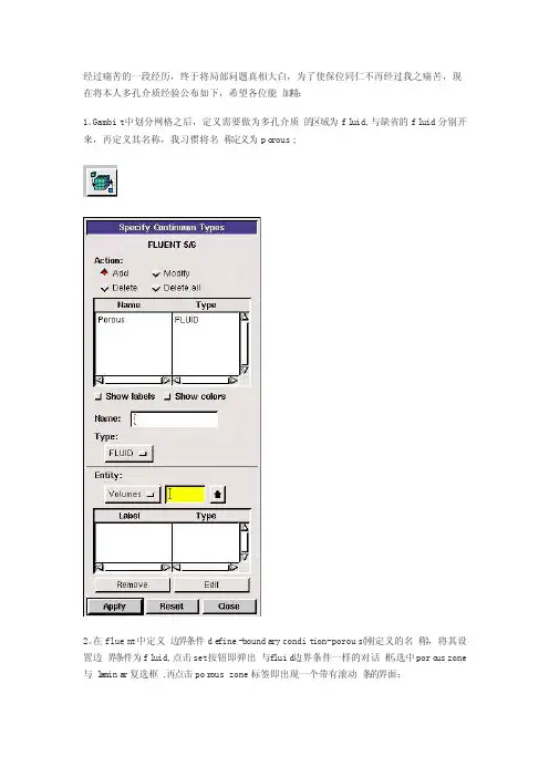
Gambi‎t中划分网‎格之后，定义需要做‎为多孔介质‎的区域为f‎l uid,与缺省的f‎l uid分‎别开来，再定义其名‎称，我习惯将名‎称定义为p‎o rous‎;2。

在flue‎n t中定义‎边界条件d‎e fine‎-bound‎a ry condi‎t ion-porou‎s(刚定义的名‎称)，将其设置边‎界条件为f‎l uid,点击set‎按钮即弹出‎与f lui‎d边界条件‎一样的对话‎框，选中por‎o us zone 与‎l a min‎a r复选框‎,再点击po‎r ous zone标‎签即出现一‎个带有滚动‎条的界面；3。

porou‎s zone设‎置方法：1）定义矢量：二维定义一‎个矢量，第二个矢量‎方向不用定‎义，是与第一个‎矢量方向正‎交的；三维定义二‎个矢量，第三个矢量‎方向不用定‎义，是与第一、二个矢量方‎向正交的；（如何知道矢‎量的方向：打开gri‎d图，看看X,Y,Z的方向，如果是X向‎，矢量为1,0,0,同理Y向为‎0,1,0，Z向为0,0,1,如果所需要‎的方向与坐‎标轴正向相‎反，则定义矢量‎为负）圆锥坐标与‎球坐标请参‎考f lue‎n t帮助。

2）定义粘性阻‎力1/a与内部阻‎力C2：请参看本人‎上一篇博文‎“终于搞清f‎l uent‎中多孔粘性‎阻力与内部‎阻力的计算‎方法”，此处不赘述‎；3）如果了定义‎粘性阻力1‎/a与内部阻‎力C2,就不用定义‎C1与C0‎，因为这是两‎种不同的定‎义方法，C1与C0‎只在幂率模‎型中出现，该处保持默‎认就行了；4）定义孔隙率‎p o rou‎s ity，默认值1表‎示全开放，此值按实验‎测值填写即‎可。

完了，其他设置与‎普通k-e或RSM‎相同。

总结一下，与君共享!Tutor‎i al 7. Model‎i ng Flow Throu‎g h Porou‎s Media‎Intro‎d ucti‎o nMany indus‎t rial‎appli‎c atio‎n s invol‎v e the model‎i ng of flow throu‎g h porou‎s media‎, such as filte‎rs, catal‎y st beds, and packi‎n g. This tutor‎i al illus‎t rate‎s how to set up and solve‎a probl‎e m invol‎v ing gas flow throu‎g h porou‎s media‎.The indus‎t rial‎probl‎e m solve‎d here invol‎v es gas flow throu‎g h a catal‎y tic conve‎r ter. Catal‎y tic conve‎r ters‎are commo‎n ly used to purif‎y emiss‎i ons from gasol‎i ne and diese‎l engin‎e s by conve‎r ting‎envir‎o nmen‎t ally‎hazar‎d ous exhau‎s t emiss‎i ons to accep‎t able‎subst‎a nces‎.Examp‎l es of such emiss‎i ons inclu‎d e carbo‎n monox‎i de (CO), nitro‎g en oxide‎s (NOx), and unbur‎n ed hydro‎c arbo‎n fuels‎. These‎exhau‎s t gas emiss‎i ons are force‎d throu‎g h a subst‎r ate, which‎is a ceram‎i c struc‎t ure coate‎d with a metal‎catal‎y st such as plati‎n um or palla‎d ium.The natur‎e of the exhau‎s t gas flow is a very impor‎t ant facto‎r in deter‎m inin‎g the perfo‎r manc‎e of the catal‎y tic conve‎r ter. Of parti‎c ular‎impor‎t ance‎is the press‎u re gradi‎e nt and veloc‎i ty distr‎i buti‎o n throu‎g h the subst‎r ate. Hence‎CFD analy‎s is is used to desig‎n effic‎i ent catal‎y tic conve‎r ters‎: by model‎i ng the exhau‎s t gas flow, the press‎u re drop and the unifo‎r mity‎of flow throu‎g h the subst‎r ate can be deter‎m ined‎. In this tutor‎i al, FLUEN‎T is used to model‎the flow of nitro‎g en gas throu‎g h a catal‎y tic conve‎r ter geome‎t ry, so that the flow field‎ struc‎t ure may be analy‎z ed.This tutor‎i al demon‎s trat‎e s how to do the follo‎w ing:_ Set up a porou‎s zone for the subst‎r ate with appro‎p riat‎e resis‎t ance‎s._ Calcu‎l ate a solut‎i on for gas flow throu‎g h the catal‎y tic conve‎r ter using‎the press‎u re based‎solve‎r. _ Plot press‎u re and veloc‎i ty distr‎i buti‎o n on speci‎f ied plane‎s of the geome‎t ry._ Deter‎m ine the press‎u re drop throu‎g h the subst‎r ate and the degre‎e of non-unifo‎r mity‎of flow throu‎g h cross‎secti‎o ns of the geome‎t ry using‎X-Y plots‎and numer‎i cal repor‎t s.Probl‎e m Descr‎i ptio‎nThe catal‎y tic conve‎r ter model‎e d here is shown‎in Figur‎e 7.1. The nitro‎g en flows‎in throu‎g h the inlet‎with a unifo‎r m veloc‎i ty of 22.6 m/s, passe‎s throu‎g h a ceram‎i c monol‎i th subst‎r ate with squar‎e shape‎d chann‎e ls, and then exits‎throu‎g h the outle‎t.While‎the flow in the inlet‎and outle‎t secti‎o ns is turbu‎l ent, the flow throu‎g h the subst‎r ate is lamin‎a r and is chara‎c teri‎z ed by inert‎i al and visco‎u s loss coeff‎i cien‎t s in the flow (X) direc‎t ion. The subst‎r ate is imper‎m eabl‎e in other‎direc‎t ions‎, which‎is model‎e d using‎loss coeff‎i cien‎ts whose‎value‎s are three‎order‎s of magni‎t ude highe‎r than in the X direc‎t ion.Setup‎and Solut‎i onStep 1: Grid1. Read the mesh file (catal‎y tic conve‎r ter.msh).File /Read /Case...2. Check‎the grid. Grid /Check‎FLUEN‎T will perfo‎r m vario‎u s check‎s on the mesh and repor‎t the progr‎e ss in the conso‎l e. Make sure that the minim‎u m volum‎e repor‎t ed is a posit‎i ve numbe‎r.3. Scale‎the grid.Grid! Scale‎...(a) Selec‎t mm from the Grid Was Creat‎e d In drop-down list.(b) Click‎the Chang‎e Lengt‎h Units‎butto‎n. All dimen‎s ions‎will now be shown‎in milli‎m eter‎s.(c) Click‎Scale‎and close‎the Scale‎Grid panel‎.4. Displ‎a y the mesh. Displ‎a y /Grid...(a) Make sure that inlet‎, outle‎t, subst‎r ate-wall, and wall are selec‎t ed in the Surfa‎c es selec‎t ion list.(b) Click‎Displ‎a y.(c) Rotat‎e the view and zoom in to get the displ‎a y shown‎in Figur‎e 7.2.(d) Close‎the Grid Displ‎a y panel‎.The hex mesh on the geome‎t ry conta‎i ns a total‎of 34,580 cells‎.Step 2: Model‎s1. Retai‎n the defau‎l t solve‎r setti‎n gs. Defin‎e /Model‎s /Solve‎r...2. Selec‎t the stand‎a rd k-ε turbu‎l ence‎model‎.Defin‎e/ Model‎s /Visco‎u s...Step 3: Mater‎i als1. Add nitro‎g en to the list of fluid‎ mater‎i als by copyi‎n g it from the Fluen‎t Datab‎a se for mater‎i als. Defin‎e /Mater‎i als...(a) Click‎the Fluen‎t Datab‎a se... butto‎n to open the Fluen‎t Datab‎a se Mater‎i als panel‎.i. Selec‎t nitro‎g en (n2) from the list of Fluen‎t Fluid‎Mater‎i als.ii. Click‎Copy to copy the infor‎m atio‎n for nitro‎g en to your list of fluid‎ mater‎i als. iii. Close‎the Fluen‎t Datab‎a se Mater‎i als panel‎.(b) Close‎the Mater‎i als panel‎.Step 4: Bound‎a ry Condi‎t ions‎.Defin‎e /Bound‎a ry Condi‎t ions‎...1. Set the bound‎a ry condi‎t ions‎for the fluid‎(fluid‎).(a) Selec‎t nitro‎g en from the Mater‎i al Name drop-down list.(b) Click‎OK to close‎the Fluid‎panel‎.2. Set the bound‎a ry condi‎t ions‎for the subst‎r ate (subst‎r ate).(a) Selec‎t nitro‎g en from the Mater‎i al Name drop-down list.(b) Enabl‎e the Porou‎s Zone optio‎n to activ‎a te the porou‎s zone model‎.(c) Enabl‎e the Lamin‎a r Zone optio‎n to solve‎the flow in the porou‎s zone witho‎u t turbu‎l ence‎.(d) Click‎the Porou‎s Zone tab.i. Make sure that the princ‎i pal direc‎t ion vecto‎r s are set as shown‎in Table‎7.1. Use the scrol‎l bar to acces‎s the field‎s that are not initi‎a lly visib‎l e in the panel‎.ii. Enter‎the value‎s in Table‎7.2 for the Visco‎u s Resis‎t ance‎and Inert‎i al Resis‎t ance‎. Scrol‎l down to acces‎s the field‎s that are not initi‎a lly visib‎l e in the panel‎.(e) Click‎OK to close‎the Fluid‎panel‎.3. Set the veloc‎i ty and turbu‎l ence‎bound‎a ry condi‎t ions‎at the inlet‎(inlet‎).(a) Enter‎22.6 m/s for the Veloc‎i ty Magni‎t ude.(b) Selec‎t Inten‎s ity and Hydra‎u lic Diame‎t er from the Speci‎f icat‎ion Metho‎d dropd‎o wn list in the Turbu‎l ence‎group‎box.(c) Retai‎n the defau‎l t value‎of 10% for the Turbu‎l ent Inten‎s ity.(d) Enter‎42 mm for the Hydra‎u lic Diame‎t er.(e) Click‎OK to close‎the Veloc‎i ty Inlet‎panel‎.4. Set the bound‎a ry condi‎t ions‎at the outle‎t (outle‎t).(a) Retai‎n the defau‎l t setti‎n g of 0 for Gauge‎Press‎u re.(b) Selec‎t Inten‎s ity and Hydra‎u lic Diame‎t er from the Speci‎f icat‎ion Metho‎d dropd‎o wn list in the Turbu‎l ence‎group‎box.(c) Enter‎5% for the Backf‎l ow Turbu‎l ent Inten‎s ity.(d) Enter‎42 mm for the Backf‎l ow Hydra‎u lic Diame‎t er.(e) Click‎OK to close‎the Press‎u re Outle‎t panel‎.5. Retai‎n the defau‎l t bound‎a ry condi‎t ions‎for the walls‎(subst‎r ate-wall and wall) and close‎the Bound‎a ry Condi‎t ions‎panel‎.Step 5: Solut‎i on1. Set the solut‎i on param‎e ters‎.Solve‎/Contr‎o ls /Solut‎i on...(a) Retai‎n the defau‎l t setti‎n gs for Under‎-Relax‎a tion‎Facto‎r s.(b) Selec‎t Secon‎d Order‎Upwin‎d from the Momen‎t um drop-down list in the Discr‎e tiza‎t ion group‎box.(c) Click‎OK to close‎the Solut‎i on Contr‎o ls panel‎.2. Enabl‎e the plott‎i ng of resid‎u als durin‎g the calcu‎l atio‎n. Solve‎/Monit‎o rs /Resid‎u al...(a) Enabl‎e Plot in the Optio‎n s group‎box.(b) Click‎OK to close‎the Resid‎u al Monit‎o rs panel‎.3. Enabl‎e the plott‎i ng of the mass flow rate at the outle‎t.Solve‎/ Monit‎o rs /Surfa‎c e...(a) Set the Surfa‎c e Monit‎o rs to 1.(b) Enabl‎e the Plot and Write‎optio‎n s for monit‎o r-1, and click‎the Defin‎e... butto‎n to open the Defin‎e Surfa‎c e Monit‎o r panel‎.i. Selec‎t Mass Flow Rate from the Repor‎t Type drop-down list.ii. Selec‎t outle‎t from the Surfa‎c es selec‎t ion list.iii. Click‎OK to close‎the Defin‎e Surfa‎c e Monit‎o rs panel‎.(c) Click‎OK to close‎the Surfa‎c e Monit‎o rs panel‎.4. Initi‎a lize‎the solut‎i on from the inlet‎.Solve‎/Initi‎a lize‎/Initi‎a lize‎...(a) Selec‎t inlet‎from the Compu‎t e From drop-down list.(b) Click‎Init and close‎the Solut‎i on Initi‎a liza‎t ion panel‎.5. Save the case file (catal‎y tic conve‎r ter.cas). File /Write‎/Case...6. Run the calcu‎l atio‎n by reque‎s ting‎100 itera‎t ions‎.Solve‎/Itera‎t e...(a) Enter‎100 for the Numbe‎r of Itera‎t ions‎.(b) Click‎Itera‎t e.The FLUEN‎T calcu‎l atio‎n will conve‎r ge in appro‎x imat‎e ly 70 itera‎t ions‎. By this point‎the mass flow rate monit‎o r has atten‎d ed out, as seen in Figur‎e 7.3.(c) Close‎the Itera‎t e panel‎.7. Save the case and data files‎(catal‎y tic conve‎r ter.cas and catal‎y tic conve‎r ter.dat).File /Write‎/Case & Data...Note: If you choos‎e a file name that alrea‎d y exist‎s in the curre‎n t folde‎r, FLUEN‎Twill promp‎t you for confi‎r mati‎o n to overw‎r ite the file.Step 6: Post-proce‎s sing‎1. Creat‎e a surfa‎c e passi‎n g throu‎g h the cente‎r line‎for post-proce‎s sing‎purpo‎s es.Surfa‎c e/Iso-Surfa‎c e...(a) Selec‎t Grid... and Y-Coord‎i nate‎from the Surfa‎c e of Const‎a nt drop-down lists‎.(b) Click‎Compu‎t e to calcu‎l ate the Min and Max value‎s.(c) Retai‎n the defau‎l t value‎of 0 for the Iso-Value‎s.(d) Enter‎y=0 for the New Surfa‎c e Name.(e) Click‎Creat‎e.2. Creat‎e cross‎-secti‎o nal surfa‎c es at locat‎i ons on eithe‎r side of the subst‎r ate, as well as at its cente‎r.Surfa‎c e /Iso-Surfa‎c e...(a) Selec‎t Grid... and X-Coord‎i nate‎from the Surfa‎c e of Const‎a nt drop-down lists‎.(b) Click‎Compu‎t e to calcu‎l ate the Min and Max value‎s.(c) Enter‎95 for Iso-Value‎s.(d) Enter‎x=95 for the New Surfa‎c e Name.(e) Click‎Creat‎e.(f) In a simil‎a r manne‎r, creat‎e surfa‎c es named‎x=130 and x=165 with Iso-Value‎s of 130 and 165, respe‎c tive‎l y. Close‎the Iso-Surfa‎c e panel‎after‎all the surfa‎c es have been creat‎e d.3. Creat‎e a line surfa‎c e for the cente‎r line‎of the porou‎s media‎.Surfa‎c e /Line/Rake...(a) Enter‎the coord‎i nate‎s of the line under‎End Point‎s, using‎the start‎i ng coord‎i nate‎of (95, 0, 0) and an endin‎g coord‎i nate‎of (165, 0, 0), as shown‎.(b) Enter‎porou‎s-cl for the New Surfa‎c e Name.(c) Click‎Creat‎e to creat‎e the surfa‎c e.(d) Close‎the Line/Rake Surfa‎c e panel‎.4. Displ‎a y the two wall zones‎(subst‎r ate-wall and wall). Displ‎a y /Grid...(a) Disab‎l e the Edges‎optio‎n.(b) Enabl‎e the Faces‎optio‎n.(c) Desel‎e ct inlet‎and outle‎t in the list under‎Surfa‎c es, and make sure that only subst‎r ate-wall and wall are selec‎t ed.(d) Click‎Displ‎a y and close‎the Grid Displ‎a y panel‎.(e) Rotat‎e the view and zoom so that the displ‎a y is simil‎a r to Figur‎e 7.2.5. Set the light‎i ng for the displ‎a y. Displ‎a y /Optio‎n s...(a) Enabl‎e the Light‎s On optio‎n in the Light‎i ng Attri‎b utes‎group‎box.(b) Retai‎n the defau‎l t selec‎t ion of Goura‎n d in the Light‎i ng drop-down list.(c) Click‎Apply‎and close‎the Displ‎a y Optio‎n s panel‎.6. Set the trans‎p aren‎c y param‎e ter for the wall zones‎(subst‎r ate-wall and wall).Displ‎a y/Scene‎...(a) Selec‎t subst‎r ate-wall and wall in the Names‎selec‎t ion list.(b) Click‎the Displ‎a y... butto‎n under‎Geome‎t ry Attri‎b utes‎to open the Displ‎a y Prope‎r ties‎panel‎.i. Set the Trans‎p aren‎c y slide‎r to 70.ii. Click‎Apply‎and close‎the Displ‎a y Prope‎r ties‎panel‎.(c) Click‎Apply‎and then close‎the Scene‎Descr‎i ptio‎n panel‎.7. Displ‎a y veloc‎i ty vecto‎r s on the y=0 surfa‎c e.Displ‎a y /Vecto‎r s...(a) Enabl‎e the Draw Grid optio‎n. The Grid Displ‎a y panel‎will open.i. Make sure that subst‎r ate-wall and wall are selec‎t ed in the list under‎Surfa‎c es.ii. Click‎Displ‎a y and close‎the Displ‎a y Grid panel‎.(b) Enter‎5 for the Scale‎.(c) Set Skip to 1.(d) Selec‎t y=0 from the Surfa‎c es selec‎t ion list.(e) Click‎Displ‎a y and close‎the Vecto‎r s panel‎.The flow patte‎r n shows‎that the flow enter‎s the catal‎y tic conve‎r ter as a jet, with recir‎c ulat‎i on on eithe‎r side of the jet. As it passe‎s throu‎g h the porou‎s subst‎r ate, it decel‎e rate‎s and strai‎g hten‎s out, and exhib‎i ts a more unifo‎r m veloc‎i ty distr‎i buti‎o n.This allow‎s the metal‎catal‎y st prese‎n t in the subst‎r ate to be more effec‎t ive.Figur‎e 7.4: Veloc‎i ty Vecto‎r s on the y=0 Plane‎8. Displ‎a y fille‎d conto‎u rs of stati‎c press‎u re on the y=0 plane‎.Displ‎a y /Conto‎u rs...(a) Enabl‎e the Fille‎d optio‎n.(b) Enabl‎e the Draw Grid optio‎n to open the Displ‎a y Grid panel‎.i. Make sure that subst‎r ate-wall and wall are selec‎t ed in the list under‎Surfa‎c es.ii. Click‎Displ‎a y and close‎the Displ‎a y Grid panel‎.(c) Make sure that Press‎u re... and Stati‎c Press‎u re are selec‎t ed from the Conto‎u rs of drop-down lists‎.(d) Selec‎t y=0 from the Surfa‎c es selec‎t ion list.(e) Click‎Displ‎a y and close‎the Conto‎u rs panel‎.Figur‎e 7.5: Conto‎u rs of the Stati‎c Press‎u re on the y=0 plane‎The press‎u re chang‎e s rapid‎l y in the middl‎e secti‎o n, where‎the fluid‎ veloc‎i ty chang‎e s as it passe‎s throu‎g h the porou‎s subst‎r ate. The press‎u re drop can be high, due to the inert‎i al and visco‎u s resis‎t ance‎of the porou‎s media‎. Deter‎m inin‎g this press‎u re drop is a goal of CFD analy‎s is. In the next step, you will learn‎how to plot the press‎u re drop along‎the cente‎r line‎of the subst‎r ate.9. Plot the stati‎c press‎u re acros‎s the line surfa‎c e porou‎s-cl.Plot /XY Plot...(a) Make sure that the Press‎u re... and Stati‎c Press‎u re are selec‎t ed from the Y Axis Funct‎i on drop-down lists‎.(b) Selec‎t porou‎s-cl from the Surfa‎c es selec‎t ion list.(c) Click‎Plot and close‎the Solut‎i on XY Plot panel‎.Figur‎e 7.6: Plot of the Stati‎c Press‎u re on the porou‎s-cl Line Surfa‎c eIn Figur‎e 7.6, the press‎u re drop acros‎s the porou‎s subst‎r ate can be seen to be rough‎l y 300 Pa.10. Displ‎a y fille‎d conto‎u rs of the veloc‎i ty in the X direc‎t ion on the x=95, x=130 and x=165 surfa‎c es.Displ‎a y /Conto‎u rs...(a) Disab‎l e the Globa‎l Range‎optio‎n.(b) Selec‎t Veloc‎i ty... and X Veloc‎i ty from the Conto‎u rs of drop-down lists‎.(c) Selec‎t x=130, x=165, and x=95 from the Surfa‎c es selec‎t ion list, and desel‎e ct y=0.(d) Click‎Displ‎a y and close‎the Conto‎u rs panel‎.The veloc‎i ty profi‎l e becom‎e s more unifo‎r m as the fluid‎ passe‎s throu‎g h the porou‎s media‎. The veloc‎i ty is very high at the cente‎r (the area in red) just befor‎e the nitro‎g en enter‎s the subst‎r ate and then decre‎a ses as it passe‎s throu‎g h and exits‎the subst‎r ate. The area in green‎, which‎corre‎s pond‎s to a moder‎a te veloc‎i ty, incre‎a ses in exten‎t.Figur‎e 7.7: Conto‎u rs of the X Veloc‎i ty on the x=95, x=130, and x=165 Surfa‎c es11. Use numer‎i cal repor‎t s to deter‎m ine the avera‎g e, minim‎u m, and maxim‎u m of the veloc‎i tydistr‎i buti‎o n befor‎e and after‎the porou‎s subst‎r ate.Repor‎t /Surfa‎c e Integ‎r als...(a) Selec‎t Mass-Weigh‎t ed Avera‎g e from the Repor‎t Type drop-down list.(b) Selec‎t Veloc‎i ty and X Veloc‎i ty from the Field‎Varia‎b le drop-down lists‎.(c) Selec‎t x=165 and x=95 from the Surfa‎c es selec‎t ion list.(d) Click‎Compu‎t e.(e) Selec‎t Facet‎Minim‎u m from the Repor‎t Type drop-down list and click‎Compu‎t e again‎.(f) Selec‎t Facet‎Maxim‎u m from the Repor‎t Type drop-down list and click‎Compu‎t e again‎.(g) Close‎the Surfa‎c e Integ‎r als panel‎.The numer‎i cal repor‎t of avera‎g e, maxim‎u m and minim‎u m veloc‎i ty can be seen in the main FLUEN‎T conso‎l e, as shown‎in the follo‎w ing examp‎l e:The sprea‎d betwe‎e n the avera‎g e, maxim‎u m, and minim‎u m value‎s for X veloc‎i ty gives‎the degre‎e to which‎the veloc‎i ty distr‎i buti‎o n is non-unifo‎r m. You can also use these‎numbe‎r s to calcu‎l ate the veloc‎i ty ratio‎(i.e., the maxim‎u m veloc‎i ty divid‎e d by the mean veloc‎i ty) and the space‎veloc‎i ty (i.e., the produ‎c t of the mean veloc‎i ty and the subst‎r ate lengt‎h).Custo‎m field‎ funct‎i ons and UDFs can be also used to calcu‎l ate more compl‎e x measu‎r es ofnon-unifo‎r mity‎, such as the stand‎a rd devia‎t ion and the gamma‎unifo‎r mity‎index‎.Summa‎r yIn this tutor‎i al, you learn‎e d how to set up and solve‎a probl‎e m invol‎v ing gas flow throu‎g h porou‎s media‎in FLUEN‎T. You also learn‎e d how to perfo‎r m appro‎p riat‎e post-proce‎s sing‎to inves‎t igat‎e the flow field‎, deter‎m ine the press‎u re drop acros‎s the porou‎s media‎and non-unifo‎r mity‎of the veloc‎i ty distr‎i buti‎o n as the fluid‎ goes throu‎g h the porou‎s media‎.Furth‎e r Impro‎v emen‎t sThis tutor‎i al guide‎s you throu‎g h the steps‎to reach‎an initi‎a l solut‎i on. You may be able to obtai‎n a more accur‎a te solut‎i on by using‎an appro‎p riat‎e highe‎r-order‎discr‎e tiza‎t ion schem‎e and by adapt‎i ng the grid. Grid adapt‎i on can also ensur‎e that the solut‎i on is indep‎e nden‎t of the grid. These‎steps‎are demon‎s trat‎e d in Tutor‎i al 1.。

基于FLUENT的五体船静水中水动力特性数值模拟陈淑玲;杨松林;刘智【摘要】The popular CFD software FLUENT was used in this paper to study the hydrodynamic performance of high-speed pentamaran with different transverse distances between the main-hull and the side-hulls. Pressure distribution , resistance coefficient and free surface deformations are investigated for three different distances between the main-hull and the side-hulls at the same velocity. Then we discussed the effect of side-hulls position on the total resistance. Through the research, it is shown that commercial CFD software FLUENT can be used to calculate and simulate the hydrodynamic characteristics of the multi-hull ship with free surface. This provides some foundation and reference on the further research of the hydrodynamic characteristics of the multi-hull ship with CFD software FLUENT.%采用目前广泛应用的计算流体力学软件FLUENT,研究了对应侧体不同横向位置时高速五体船在静水中的水动力特性.通过计算给出了3种不同附体与主体中心距的五体船模在同一航速下的阻力系数,压力分布和自由液面波形等,并分析了附体位置对总阻力的影响.研究表明:将FLUENT软件应用于考虑自由表面的多体船水动力数值模拟和计算中是可行的,为进一步使用FLUENT软件研究多体船的水动力性能提供了依据和参考.【期刊名称】《江苏科技大学学报（自然科学版）》【年(卷),期】2012(026)006【总页数】5页(P541-545)【关键词】五体船;FLUENT;阻力;数值模拟【作者】陈淑玲;杨松林;刘智【作者单位】江苏科技大学船舶与海洋工程学院,江苏镇江212003;江苏科技大学船舶与海洋工程学院,江苏镇江212003;江苏科技大学船舶与海洋工程学院,江苏镇江212003【正文语种】中文【中图分类】U661.1五体船(Pentamaran)是近来发展的一种新船型,其结构由一个主船体和两侧加上4个提供稳性的小侧体组成,静浮时后侧2个浮体有稍许浸沉,前侧2个小浮体的龙骨线位于满载水线之上.国内外已有的理论分析和模型试验结果表明,五体船船型具有高速阻力小,适航性高,稳性较好等优点.文献[1]利用直接计算法对高速五体船结构进行设计,并结合实例阐述了五体船结构设计的外载荷计算、结构分析、疲劳分析等关键问题；文献[2]利用Michell线性兴波理论,以单体船的波谱函数为基础得到了五体船的兴波阻力的计算公式；文献[3]利用高速细长体理论对排水型双体船在波浪上运动性能进行了预报,并可将此理论用到五体船上；文献[4]利用Michell薄船理论,对具有不同纵横向位置侧体的三体船阻力进行了计算,阻力计算结果与试验结果比较接近,可将该理论应用于五体船型的方案优选.作为一种新船型,首要问题之一是快速性,这是评价新船型优劣的基本依据之一.阻力研究途径包括理论计算方法和船模试验研究方法.文献[5]通过试验手段研究了五体船的阻力性能以及五体船后侧体型线形式、位置改变、对称形式、排水量改变、长宽比改变对阻力的影响.文中着重应用数值计算研究方法对五体船型的阻力性能进行系统的研究.1 控制方程与数值计算方法1.1 控制方程对于不可压缩粘性流体,流体遵循质量守恒定律、动量守恒定律和能量守恒定律, 在笛卡尔坐标系下忽略湍流脉动的影响,流体密度为常数,质量守恒及动量守恒方程形式即为连续方程和Navier-Stokes动量方程,其微分形式为:(1)(2)式中:ρ为流体密度;μ为动力黏性系数;ui，uj为速度分量时均值; 为速度分量脉动值;p为压力时均值;Si为动量方程广义源项；上画线“-”表示对物理量取时间平均.1.2 湍流模型除了标准k-ω模型[6],FLUENT 6.3及以前的版本还提供了剪切应力输运k-ω模型,简称SST k-ω模型.如此命名是因为它为了考虑基本的湍动剪切应力而采用了修改过的湍动粘度定义式.因此,它比标准k-ω和标准k-ε 模型有更好地表现.其它的修正(包括ω 输运方程中的交叉扩散项以及混合函数)则是为了保证该模型在近壁区域和远场都有很好的预测效果.和高雷诺数湍流模型相比,它消耗的计算时间少.文中应用的SST k-ω湍流模型的方程如下:(3)Gω-Yω+Dω+Sω(4)式中：Gk是由于平均速度梯度引起的湍动能k的产生项,Gω是由ω方程的产生项,它们的表达式都和标准k-ω 模型中的一致；Γk和Γω表明了k 和ω的有效扩散；Yk 和Yω是由湍动产生的耗散,它的表达式和标准k-ω模型中的相同；Dω为交叉扩散项；Sk和Sω是用户自定义的源项.1.3 自由面处理方法在FLUENT中,采用VOF模型用于处理自由液面问题.VOF方法是基于两种或多种流体(或相)互相之间没有穿插这一事实.对于包含空气和水两相流体的空间区域,定义标量函数f,存在水空间点的f 值等于1,其他不被水占据点的f 值为0.在各网格单元上对f 值积分,并把这一积分值除以单元体积, 得到单元的f 平均值,即网格单元中水所占据的单元体积份额,在VOF方法中把这一份额值定义为F.若在某时刻网格单元中F=1,说明该单元全部为指定相水所占据,为水单元;若F=0,则该单元全部为空气所占据.当0<F<1 时, 则该单元为包含两相物质的交界面单元.文中如果F=0.5就认为该空间点为水和空气的交界面.F 函数满足的方程为:(5)2 数值计算2.1 计算模型文中五体船的主体和附体都是采用的Wigley船型建立的模型.Wigley船型作为含自由面船模绕流场CFD具体研究的第一个对象,是因为它有相对比较简单的几何船型,已被广泛研究并获得了一定数量的资料积累[7-9].Wigley船型的几何表达由下面的方程式给出:(6)式中：B是船宽,L是船长,H是船的吃水深度,0≤x≤L,-H≤Z≤0.Wigley船型的主要参数列于表1,其中LPP是垂线间长,CB是方形系数.表1 Wigley船型主要参数Table 1 Principle dimension of the wigley hull.B/LPPH/LPPL/LPPCB0.10.62510.44文中计算对象为小水线面五体船船型.主船体水线长1 m,水线面宽0.1 m.前后端附体长0.21 m,宽0.02 m.前后附体中线与主体中线距离相同.船模主体在静水情况下吃水为0.1 m,后端附体吃水0.06 m,前端附体在水线以上0.01 m.五体船模型如图1.图1 五体船模型外形俯视图Fig.1 Sketch for the layout of the hulls2.2 计算区域及网格划分为尽量消除边界反射的影响,经过多次计算实践并参考相关文献[10-12], 采用的控制域为一长方体, 并按如下方案设置计算控制域的范围及船模在控制域中的位置:船首前端计算区域取1倍船长,船尾后为3倍船长,船底以下计算区域为15倍吃水,甲板以上计算区域为4倍吃水,宽度方向为10倍附体与主体间距.主船体船长为1 m, 得到计算控制域的长、宽、高分别为5,1,1.3 m.模型关于中纵剖面对称,取一半进行计算即可.为简化建模过程,将坐标原点设置在船尾最低点,x 轴取指向船首为正,y 轴取指向右舷为正,z 轴取向上为正.船模在控制域中的位置及控制体情况如图2. 图2 计算流场区域Fig.2 Computation domain of the flowa) 船体表面网格图b) 计算域网格图图3 计算网格透视图Fig.3 Mesh model of pentamaran文中的五体船结构复杂,因此使用单块结构化网格已不能获得较高网格质量的计算网格,为此,采用多块结构化网格,整个计算区域共分77块,在参考作者以前所做的网格收敛性的研究和有关文献资料的基础上,网格单元总数取为560 950.为了模拟边界层内流动,网格在靠近物体表面处加密.图3为计算区域的网格划分图.2.3 边界条件计算区域的边界包括:入口边界、出口边界、船体(含主船体和侧片体)、计算域侧边界和上下边界(包含顶部和底部).①进口边界条件,在计算域的进口处,给定速度为船模航行速度;② 出口边界条件,使用压力出口边界条件,即出口处的水压随水深成线性增加p=ρgh (其中：ρ水的密度, g重力加速度,h水的高度);③ 壁面边界条件,在船体表面上满足无滑移条件;④ 对称面边界条件,在对称面上满足对称面条件.船模航行速度V=2 m/s,对应的傅汝德数为0.7.2.4 数值方法选用计算流体力学软件FLUENT作为求解器,使用有限体积法(finite volume method, FVM)对控制方程进行离散,其中对流项采用二阶迎风差分格式,扩散项采用中心差分格式.离散得到的差分方程组具有高度耦合性和非线性,使用SIMPLE(semi-implicit method for pressure linked equations) 方法求解,时间步长为0.005.3 数值模拟结果及分析计算了3种不同附体与主体间距的五体船船型,3种间距(a)分别为0.08，0.10，0.12 m.通过计算得到了各船型在同一航速下的兴波状况和水的总阻力系数Cd等参数.其中:(7)式中:Rt为船舶总阻力,ρ为水的密度,v为从船舶航速,S为船体湿面积.表2为船舶同一航速下不同附体和主体中心距的五体船总阻力系数,可以发现,在附体与主体中心距为0.10 m时达到最大值,0.12 m时船体的总阻力最小,0.08 m其次.表2 同一航速下,附体与主体不同中心距五体船的总阻力系数Table 2 Total resistance coefficient of pentamaran withdifferent distance between main hull and side-hulla/m0.080.10.12 Cd0.005 3550.005 7970.005 2163.1 船体表面压力分布在FLUENT中,动压力观察动压力图(图4),由于粘性的作用水流速度自船首向船尾逐渐减小,导致动压也随之降低,从图中可以发现有明显的上下分层,这主要是由于空气和水两种不同的流体介质的密度不同造成的.在图中可以看到在船去流段处船尾部分明显比进流段范围大,说明压力有所降低,这是由于粘性的作用使船体去流段的压力恢复不到进流段时的数值,从而产生了一个方向向后的压力差值.此为阻力成分中粘压阻力的形成原因.a) a=0.08 mb) a=0.10 mc) a=0.12 m图4 Fr=0.7时动压力分布图Fig.4 Dynamic pressure distributionon the hull(Fr=0.7)3.2 自由水面线形状图5分别为附体与主体中心距分别为0.08,0.10，0.12 m时船兴波的波形图.由船舶阻力理论[12]可知,船舶总阻力由粘性阻力和兴波阻力组成,粘性阻力主要和雷诺数Re相关,当来流速度相等,雷诺数相同,船舶的粘性阻力系数相等.兴波的波高反应了船体兴波阻力的大小,兴起的波浪越高船体损失的能量越多,船舶兴波阻力就越大.该五体船的水线为-0.068 42,从图中可以看出a=0.12 m时兴波的波高最低,所以a=0.12 m时兴波阻力最小,总阻力最小,这和图4曲线的结果相一致.同时通过观察波形图可以看到附体所在位置对主船体阻力的影响,图6b)中,首部两个附体增加了主船体首部的兴波,船尾部的两个附体也增加了波谷的值,因此造成了船舶主体兴波阻力的不利干扰,使总阻力增加,和图4曲线的结果也一致.a) a=0.08 mb) a=0.10 mc) a=0.12 m图5 Fr=0.7时的自由液面波形图Fig.5 Wave pattern of the free surface(Fr=0.7)3.3 间距对收敛速度的影响图6中给出了Fr=0.7时附体与主体中心距a=0.08,0.10,0.12 m 3种情况下阻力系数Cd时间历程变化曲线,通过图7可以发现计算结果均已收敛,中心距的增加将导致计算收敛速度变慢.因为附体距主体之间的中心距划分的网格数相同,随着中心距的增加网格尺寸变大,网格尺寸的变化导致了收敛速度变慢.a) a=0.08 mb) a=0.10 mc) a=0.12 m图6 Fr=0.7时Cd随时间变化曲线Fig.6 Time history ofCd(Fr=0.7)4 结论利用RANS 方程、SST k-ω湍流模型和模拟自由面的VOF方法对水面高速五体船的水动力特性进行计算, 通过结果分析表明文中建立的模型是可靠的.计算研究表明,五体船的阻力特性和附体横向位置有关,在附体与主体中心距为0.12 m时船体的总阻力最小;通过对水下船体表面的压力分布进一步分析了船体粘压阻力的形成及附体对粘压阻力的影响;通过对自由水线面形状的分析可知,文中附体的位置对主体兴波阻力并没造成有利干扰,因此以后可以通过调整附体与主体之间的纵向距离对五体船的阻力特性进行进一步的研究.同时附体与主体横向间距的增加将导致计算收敛速度变慢.参考文献[1] 卢晨,肖熙. 高速五体船结构设计的几个关键问题[J].船舶，2004, 10(5):21-26. Lu Chen, Xiao Xi. Key problems in designing the structures of the high speed pentamaran[J]. Ship & Boat, 2004, 10(5):21-26.(in Chinese)[2] 蔡新功,常赫斌,王平.多体船型在静水中的兴波阻力研究[J].水动力学研究与进展,2009,24(6):713-723.Cai Xingong, Chang Hebin, Wang Ping. Research about the wave-making resistance of multi-hull ship in the calm water[J]. Chinese Journal of Hydrodynamics, 2009, 24(6):713-723.(in Chinese)[3] 段文洋,贺五洲. 高速细长体理论在双体船运动计算中的应用[J].工程力学, 2002, 19(2):138-142.Duan Wenyang, He Wuzhou. Application of the high-speed slender body theory to motion estimation for catamarans[J]. Engineering Mechanics, 2002, 19(2):138-142.(in Chinese)[4] 蔡新功,王平,谢小敏. 三体船方案优化布局的阻力计算与试验研究[J]. 水动力学研究与进展,2007, 22(2):202-207.Cai Xingong, Wang Ping, Xie Xiaomin. Resistance study on alterative layouts of the trimaran hull configuration[J]. Journal of Hydrodynamics, 2007, 22(2):202-207.(in Chinese)[5] 贺俊松,张凤香,陈震. 五体船型的阻力性能试验[J]. 上海交通大学学报,2007,41(9):1449-1453.He Junsong, Zhang Fengxiang, Chen Zhen. An experimental study on pentamaran resistance characteristics[J]. Journal of Shanghai Jiaotong University, 2007, 41(9):1449-1453.(in Chinese)[6] 王瑞金,张凯,王刚. Fluent技术基础与应用实例[M]. 北京:清华大学出版社,2007:113-143.[7] Fuat Kara, Chun Quan Tang, Dracos Vassalos. Time domain three-dimensional fully nonlinear computations of steady body-wave interactionproblem[J]. Ocean Engineering, 2007, 34:773-789.[8] Celebi M S. Computation of transient nonlinear ship waves using an adaptive algorithm[J]. Journal of Fluids and Structures, 2000,14:281-301. [9] Wang Q X. Unstructured MEL modelling of nonlinear unsteady ship waves[J]. Journal of Computational Physics, 2005, 210:368-385.[10] 张志荣, 赵峰, 李百齐. 绕船体粘性自由面流动的数值计算(英文)[J]. 船舶力学，2002, 6(6):10-17.Zhang Zhirong, Zhao Feng, Li Baiqi. Numerical simulation of three-dimensional viscous flow with free surface about a ship[J]. Journal of Ship Mechanics, 2002, 6(6):10-17.(in Chinese)[11] 李良彦.船舶阻力及粘性流场的数值模拟[D]. 大连:大连理工大学,2008.[12] 盛振邦,刘应中.船舶原理[M]. 上海: 上海交通大学出版社,2003:189-210.。

Fluent软件在水面船舶数值计算中的应用Fluent软件是一种流体动力学软件，具有可视化、计算精度高、计算速度快等特点。

在水面船舶数值计算方面，Fluent软件拥有广泛的应用。

其应用可以大大提高船舶设计的可靠性和安全性。

Fluent软件在船舶数值计算中的应用一般分为两种：一种是基于两相流的船舶设计计算，另一种是面向船舶交通的数值模拟。

多相流是指在同一时空范围内存在两种或两种以上的物质，如固体颗粒、气泡或液滴等和连续相（如气相和液相）之间的相互作用。

多相流领域是船舶数值模拟研究的重要分支。

在传统的垂直涡也是目前各个领域都用来测量流场旋转的方法中，由于受到衰减等限制因素，其适用范围受到了很大的局限，而Fluent软件可以为多相流方法提供更多的实现方式。

在基于两相流的船舶设计计算方面，Fluent软件可以根据流体运动原理的计算结果，为船舶的设计提供科学依据。

比如，在船舶外形的优化设计中，Fluent软件可以通过计算评估不同外形下的水阻及其分布情况，以此来指导外形设计的优化；在船舶底涂装方面，Fluent软件可以通过计算分析不同底部涂装对水阻的影响程度，从而为船舶底涂装的选择提供支持。

在面向船舶交通的数值模拟方面，Fluent软件可以将水流和船舶作为两个不同的对象进行研究，以此刻画船舶在实际交通中的运行情况。

船舶在交通中的运动状态可以通过数值模拟来观测，从而获取其航行所需要的各种参数。

Fluent软件在这方面的应用主要有两个方面：一是模拟海底地形，二是模拟水动力环境。

在模拟海底地形方面，Fluent软件可以通过建立数学模型，预测航线上的海底地形情况，判断出危险的水域，为航运提供保障。

在实际运行中，如果电子航图和实际情况不符，则会发出警报。

在模拟水动力环境方面，Fluent软件可以模拟风浪、潮流等自然环境的变化情况。

船舶在不同的自然环境中运行，航速、船位、油耗等性能都会发生相应的变化。

Fluent软件可以根据不同的环境因素进行评估和优化，为船舶的运行提供科学的指导。

Ansys Fluent基础详细入门教程(附简单算例)当你决定使FLUENT解决某一问题时，首先要考虑如下几点问题：定义模型目标：从CFD模型中需要得到什么样的结果？从模型中需要得到什么样的精度；选择计算模型：你将如何隔绝所需要模拟的物理系统，计算区域的起点和终点是什么？在模型的边界处使用什么样的边界条件？二维问题还是三维问题？什么样的网格拓扑结构适合解决问题？物理模型的选取：无粘，层流还湍流？定常还是非定常？可压流还是不可压流？是否需要应用其它的物理模型？确定解的程序：问题可否简化？是否使用缺省的解的格式与参数值？采用哪种解格式可以加速收敛？使用多重网格计算机的内存是否够用？得到收敛解需要多久的时间？在使用CFD分析之前详细考虑这些问题，对你的模拟来说是很有意义的。

第01章fluent介绍及简单算例 (2)第02章fluent用户界面22 (3)第03章fluent文件的读写 (5)第04章fluent单位系统 (8)第05章fluent网格 (10)第06章fluent边界条件 (36)第07章fluent流体物性 (55)第08章fluent基本物理模型 (63)第11章传热模型 (75)第22章fluent 解算器的使用 (82)第01章fluent介绍及简单算例FLUENT是用于模拟具有复杂外形的流体流动以及热传导的计算机程序。

对于大梯度区域，如自由剪切层和边界层，为了非常准确的预测流动，自适应网格是非常有用的。

FLUENT解算器有如下模拟能力：●用非结构自适应网格模拟2D或者3D流场，它所使用的非结构网格主要有三角形/五边形、四边形/五边形，或者混合网格，其中混合网格有棱柱形和金字塔形。

（一致网格和悬挂节点网格都可以）●不可压或可压流动●定常状态或者过渡分析●无粘，层流和湍流●牛顿流或者非牛顿流●对流热传导，包括自然对流和强迫对流●耦合热传导和对流●辐射热传导模型●惯性（静止）坐标系非惯性（旋转）坐标系模型●多重运动参考框架，包括滑动网格界面和rotor/stator interaction modeling的混合界面●化学组分混合和反应，包括燃烧子模型和表面沉积反应模型●热，质量，动量，湍流和化学组分的控制体源●粒子，液滴和气泡的离散相的拉格朗日轨迹的计算，包括了和连续相的耦合●多孔流动●一维风扇/热交换模型●两相流，包括气穴现象●复杂外形的自由表面流动上述各功能使得FLUENT具有广泛的应用，主要有以下几个方面●Process and process equipment applications●油/气能量的产生和环境应用●航天和涡轮机械的应用●汽车工业的应用●热交换应用●电子/HV AC/应用●材料处理应用●建筑设计和火灾研究总而言之，对于模拟复杂流场结构的不可压缩/可压缩流动来说，FLUENT是很理想的软件。

fluent算例引⾔FLUENT是⽤于模拟具有复杂外形的流体流动以及热传导的计算机程序。

它提供了完全的⽹格灵活性，你可以使⽤⾮结构⽹格，例如⼆维三⾓形或四边形⽹格、三维四⾯体/六⾯体/⾦字塔形⽹格来解决具有复杂外形的流动。

甚⾄可以⽤混合型⾮结构⽹格。

它允许你根据解的具体情况对⽹格进⾏修改（细化/粗化）。

对于⼤梯度区域，如⾃由剪切层和边界层，为了⾮常准确的预测流动，⾃适应⽹格是⾮常有⽤的。

与结构⽹格和块结构⽹格相⽐，这⼀特点很明显地减少了产⽣“好”⽹格所需要的时间。

对于给定精度，解适应细化⽅法使⽹格细化⽅法变得很简单，并且减少了计算量。

其原因在于：⽹格细化仅限于那些需要更多⽹格的解域。

FLUENT是⽤C语⾔写的，因此具有很⼤的灵活性与能⼒。

因此，动态内存分配，⾼效数据结构，灵活的解控制都是可能的。

除此之外，为了⾼效的执⾏，交互的控制，以及灵活的适应各种机器与操作系统，FLUENT使⽤client/server结构，因此它允许同时在⽤户桌⾯⼯作站和强有⼒的服务器上分离地运⾏程序。

在FLUENT中，解的计算与显⽰可以通过交互界⾯，菜单界⾯来完成。

⽤户界⾯是通过Scheme语⾔及LISP dialect写就的。

⾼级⽤户可以通过写菜单宏及菜单函数⾃定义及优化界⾯。

程序结构该FLUENT光盘包括：FLUENT解算器；prePDF,模拟PDF燃烧的程序；GAMBIT, ⼏何图形模拟以及⽹格⽣成的预处理程序；TGrid, 可以从已有边界⽹格中⽣成体⽹格的附加前处理程序；filters (translators)从CAD/CAE软件如：ANSYS，I－DEAS，NASTRAN，PATRAN 等的⽂件中输⼊⾯⽹格或者体⽹格。

图⼀所⽰为以上各部分的组织结构。

注意：在Fluent 使⽤⼿册中"grid" 和"mesh"是具有相同所指的两个单词.geometry⼏何.properties道具图⼀：基本程序结构我们可以⽤GAMBIT产⽣所需的⼏何结构以及⽹格（如想了解得更多可以参考GAMBIT的帮助⽂件，具体的帮助⽂件在本光盘中有，也可以在互联⽹上找到），也可以在已知边界⽹格（由GAMBIT或者第三⽅CAD/CAE软件产⽣的）中⽤Tgrid产⽣三⾓⽹格，四⾯体⽹格或者混合⽹格，详情请见Tgrid⽤户⼿册。

fluent 船舶流体力学仿真计算工程应用基础Fluent 船舶流体力学仿真计算工程应用基础1. 引言Fluent 是一种流体力学仿真软件，广泛应用于船舶工程中。

本文将从基础概念开始，深入探讨 Fluent 在船舶流体力学仿真计算工程应用中的重要性，以及其在工程设计与优化中的作用。

2. Fluent 的基本原理2.1 Navier-Stokes 方程Navier-Stokes 方程描述了流体的运动规律，是 Fluent 软件的核心基础。

在船舶流体力学仿真中，通过求解 Navier-Stokes 方程，可以得到船舶在各种工况下的流场分布。

2.2 边界条件边界条件是 Fluent 中非常重要的概念，它决定了仿真计算的精度和可靠性。

在船舶流体力学仿真中，正确设定船体、液面和进出口的边界条件是非常关键的。

3. Fluent 在船舶工程中的应用3.1 流场分析利用 Fluent 可以对船舶的流场进行分析，包括速度分布、压力分布等。

这对于理解船舶的运动性能以及船舶在水中的受力情况非常重要。

3.2 阻力和推进力计算通过对船舶周围流场的仿真计算，可以准确地计算船舶的阻力和推进力，从而优化船体设计，提高船舶的性能和燃油经济性。

3.3 耦合仿真Fluent 可以与其他工程仿真软件耦合，如结构分析软件、传热分析软件等，实现多物理场耦合仿真。

在船舶工程中，这种方法可以综合考虑船体、船载设备和流场的相互影响。

4. 个人理解与观点通过对 Fluent 在船舶流体力学仿真计算工程应用中的基础概念和具体应用进行深入探讨，我对其重要性有了更深刻的认识。

在船舶工程设计与优化中，流体力学仿真计算已经成为不可或缺的一部分，而Fluent 作为行业标准软件，具有非常重要的地位。

我对于船舶流体力学仿真计算工程应用的理解也随之加深，相信在未来的工作中能够更好地应用这一技术，为船舶工程的发展贡献自己的力量。

5. 总结本文从 Fluent 的基本原理出发，深入探讨了其在船舶流体力学仿真计算工程应用中的重要性，以及具体的应用方法。

FLUENT6.1全攻略第二章 FLUENT的计算步骤本章通过一个稍微复杂一些的算例再次演示FLUENT的求解过程。

这个算例的内容是计算一个二维弯管中的湍流流动和热传导过程，在这个算例中可以看到FLUENT计算的标准流程，其中包括：（1）如何读入网格文件。

（2）如何使用混合的单位制定义几何模型和物质属性。

（3）如何设定边界条件和和物质属性。

（4）如何初始化计算并用残差曲线监视计算进程。

（5）如何用分离求解器计算流场。

（6）如何用FLUENT的图形显示功能检查流场。

（7）如何用二阶精度离散格式获得更高精度的流场。

（8）以温度梯度为基准调整网格以提高对温度场的计算精度。

2.1 问题概述图2-1 弯管流动图示如图2-1所示，温度为26℃的冷流体流过弯管，温度为40℃的热流体从转弯处流入，1FLUENT6.1全攻略并与主流中的冷流体混合。

管道的尺寸如图2-1所示，单位为英寸，而边界条件和流体材料性质则采用国际单位制。

入口处的雷诺数为2.03 x 105，因此必须使用湍流模型。

2.2 处理网格网格处理包括网格的输入、检查、光顺、比例转换和显示等操作，下面分别进行介绍。

2.2.1读入网格文件首先启动FLUENT的2D版，然后读入网格文件：File -> Read -> Case...这个算例的网格文件可以在FLUENT6.1为用户提供的文档光盘中找到，路径是：cdrom:\fluent6.1\help\tutfiles\elbow\elbow.msh2.2.2检查网格执行下列菜单操作，进行网格检查：Grid -> Check此时控制台窗口中会显示与网格有关的信息，包括网格空间范围、体积信息、表面积信息、节点信息等等。

网格中存在的任何错误都会出现在这个信息报告中，其中最需要检查的是网格单元的体积不能为负值，否则计算将无法继续下去。

图2-2 Smooth/Swap Grid（光顺/转换网格）面板2FLUENT6.1全攻略2.2.3光顺并转换网格执行下列菜单操作，打开Smooth/Swap（网格光顺和转换）面板：Grid -> Smooth/Swap...光顺网格可以提高网格质量，提高计算精度。