GMM Estimation

gmm估计方法stataGMM 估计方法是一种参数估计方法，它是广义矩估计法的一种特殊形式。

GMM 估计方法通过构造题目中的未知参数的样本矩来估计参数，这种方法可以通过软件 Stata 实现。

在 Stata 中进行 GMM 估计方法，首先需要使用 gmm 命令进行设置。

gmm 命令的基本设置格式如下：gmm depvar (instrum:list varlist) [, option]其中，depvar 是被解释变量，instrum 是工具变量，option 表示其他设置选项。

GMM 估计方法的两个重要参数是工具变量和矩阵权重矩阵。

在Stata 中，可以使用ivregress 命令来生成工具变量。

同时，Stata 还提供了弱工具变量下的优化算法，用户可以通过 ivreg2 命令进行设置。

在进行 GMM 估计方法之前，需要先确定样本矩的形式，并确定权重矩阵的构造方式。

对于 GMM 估计方法的权重矩阵，可以使用被广泛引用的认可的经验记述变量或等权重矩阵来构建。

根据样本数据的特征，选择一种合适的矩阵会产生更精确的估计结果。

在实际应用中，GMM 估计方法可以用于计算模型的峰值位置、变化趋势及其他未知参数。

这种方法在金融学、计量经济学、卫生经济学、国际贸易和宏观经济政策等领域得到广泛应用。

在 Stata 中，通过对gmm 命令中 option 等参数进行设置，可以轻松完成 GMM 估计方法的计算。

总之，GMM 估计方法是一种重要的参数估计方法，Stata 软件的GMM 模块提供了实现该方法的便利性。

无论是在学术研究还是实践应用中，这种方法都拥有广泛应用前景。

generalized method of moments estimator -回复什么是广义矩估计法？广义矩估计法（Generalized Method of Moments，简称GMM）是一种用于估计经济模型参数的统计方法。

它是由经济学家Lars Peter Hansen和Thomas J. Sargent于1982年提出的。

GMM的基本思想是通过找到一个或多个矩条件来估计模型参数，其中矩条件是指对于一组给定的数据，模型预测的矩的理论值与实际观测值之间的差异。

GMM的核心是通过最小化模型预测矩与实际观测矩之间的差异来估计模型参数。

为了做到这一点，GMM引入了一个被称为矩条件函数（moment condition function）的函数，用于度量模型预测矩与观测矩之间的距离。

这个函数通常被定义为预测矩与观测矩之差的平方的加权和。

通过最小化矩条件函数，GMM可以找到最优的模型参数估计。

GMM的估计过程可以分为以下几个步骤：1. 确定模型的矩条件：首先，需要确定经济模型的矩条件，即模型的理论预测的矩与实际观测值之间的关系。

这些矩条件通常是经济模型的一些基本性质，如均值、方差、相关系数等。

2. 构建矩条件函数：根据确定的矩条件，构建矩条件函数，用于衡量模型的预测矩与实际观测矩之间的差异。

通常，矩条件函数是预测矩与观测矩之差的平方的加权和。

3. 选择权重矩阵：为了在估计模型参数时，合理地权衡不同矩条件的重要性，需要选择一个权重矩阵。

这个权重矩阵可以反映出不同矩条件的可信度或重要性。

常用的选择方法包括矩方差估计和最小二乘估计。

4. 最小化矩条件函数：使用所选择的权重矩阵和确定的矩条件函数，通过最小化矩条件函数来估计模型参数。

这个最小化过程可以使用各种数值优化算法来实现，如牛顿法、梯度下降法等。

5. 估计参数的标准误差：一旦模型参数估计得到，还需要对估计结果进行统计推断，以获得参数估计的精确度。

通常采用的方法是计算参数估计的标准误差，以衡量估计结果的波动性。

在过去的三十多年里特别是从汉森（1982）的一篇富有开创性的论文起，兴起了使用GMM 估计量的宏观经济和微观经济研究，GMM 流行的原因有两点：一是它包括了许多常用的估计量，并且为比较和评价它们提供了有用的框架；二是相对其他估计量来说，GMM 提供了一种相对“简单”的备选方法，特别是在极大似然估计量难以写出时，其优势更加凸显出来。

下面就GMM 估计量的特点和其与最小二乘法估计、极大似然估计的区别加以阐述。

（一）GMM 估计量的特点经典矩估计方法（Methods of Moments Estimation ，简称MME ）的基本思想是对样本矩与相应的概率分布模型的总体矩进行匹配。

而在很多经济理论中，比如估计动态资产定价模型的未知参数时，并没有给出随机变量的联合概率分布，而是根据已有经济理论或者先验信息给出关于一个总体正交性条件的论断，这个正交性条件通常表达为(,)0E ［g y X ，］θ=，其中()·g 是数据,（y X ）和参数θ的某个连续函数，这则构成了GMM 的基本约束及核心假设。

汉森（1982）指出，GMM 估计可以利用如下的样本矩函数来定义：T t t=1g(x ,θ)1T g （）T θ≡∑，二次型是T T TS （）Tg （）Wg （）θθθ≡'，其中W 是正定矩阵。

GMM 估计量θ使TS （）θ最小化。

在大样本条件下，GMM 估计量T θ具有一致性和渐进无偏性，并且在对t g （x ，）θ的稍加限制时，它是渐近正态分布的。

正如前面给出的，该检验对于随机过程x t 允许更为普遍的随机时间相依性。

此外，汉森还定义了渐近协方差矩阵：T t j j Eg （）g （）θθ∞-=-∞Ω≡'∑，并利用其倒数作为加权矩阵，派生出渐近正态分布，即W=Ω-1，这个选择可以确保所得到的估计量T θ（从矩阵的角度）能将其渐近协方差矩阵最小化。

汉森对Ω的估计构建是基于检验样本的一致估计，但同时θ对有效估计需要用到对Ω的估计值。

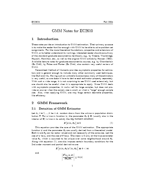
EC2610Fall2004 GMM Notes for EC26101IntroductionThese notes povide an introduction to GMM estimation.Their primary purpose is to make the reader familiar enough with GMM to be able to solve problem set assignments.For the more theoretical foundations,properties and extensions of GMM,or to better understand its workings,interested reader should consult any of the standard graduate econometrics textbooks,e.g.,by Greene,Wooldridge, Hayashi,Hamilton,etc.,as well as the original GMM article by Hansen(1982). Available lecture notes for graduate econometrics courses,e.g.by Chamberlain (Ec2140),by Pakes and Porter(Ec2144),also contain very useful reviews of GMM.Generalized Method of Moments provides asymptotic properties for estima-tors and is general enough to include many other commonly used techniques, like OLS and ML.Having such an umbrella to encompass many of the estimators is very useful,as one doesn’t have to derive each estimator property separately. With such a wide range,it is not surprising to see GMM used extensively,but one should also be careful when it is appropriate to apply.Since GMM deals with asymptotic properties,it works well for large samples,but does not pro-vide an answer when the samply size is small,or what is"large"enough sample size.Also,when applying GMM,one may forgo certain desirable properties, like e…iciency.2GMM Framework2.1De…nition of GMM EstimatorLet x i;i=1;:::;n be i.i.d.random draws from the unknown population distri-bution P.For a known function ;the parameter 02 (usually also in the interior of )is known to satisfy the key moment condition:E[(x i; 0)]=0(1)This equation provides the core of the GMM estimation.The appropriate function and the parameter 0are usually derived from a theoretical model. Both and 0can be vector valued and not necessarily of the same size.Let the size of be q,and the size of be p.The mean is0only at the true parameter value 0,which is assumed to be unique over some neighborhood around 0: Along with equation(1),one also imposes certain boundary conditions for the 2nd order moment and partial derivative one:E (x i; 0)0(x i; 0) <1and@2j(x; )@ k@ l m(x)1EC2610Fall2004 for all 2 ;where E[m(x)]<1:Also,de…neD E @ (x i; 0)@ 0and assume,D has rank equal to p,the dimension of :(Note:the above conditions are su¢cient,and properties of GMM estimators can also be obtained under weaker conditions).The task of the econometrician lies in obtaining estimate b of 0from the key moment condition.Since there is sample of size n from the population distribution,one may try to obtain the estimate by replacing the population mean with a sample one:1X i(x i;b )=0(2)This is a system of q equations with p unknowns.If p=q,we’re"just-identi…ed,"and under some weak conditions,one can obtain a(unique)solution to(2)around the neighborhood of 0.When q>p,then we’re"over-identi…ed," and a solution will not exist for most functions :A natural approach for the latter case might be to try to get the left hand side as close to0as possible,with"closeness"de…ned over some norm k kA n:k y k A n=y0A 1n ywhere A n is q-by-q symmetric,positive de…nite matrix.Another approach could be to…nd the soltuion to(2),by making some linear combination of j equations equal to0.I.e.for some p-by-q matrix C n,of rankp,solve for:C n 1n X i(x i;b )=0(3)which will give us p equations with p unknowns.In fact,both approaches are equivalent and GMM estimation is setup to do exactly that.That is,when p=q,GMM is just-identi…ed and we can usually solve for b exactly.When q>p,we’re in the over-identi…ed case and for some appropriate matrix A n(or C n),GMM estimate b is found by:b =arg min 2 "1n X i(x i; )#0A 1n"1n X i(x i; )#(4)(Or equivalently,solving for:equation(3)).The choice of A n will be discussed later,but for now assume A n ! a.s.,where is also symmetric and positive-de…nite.2.2Asymptotic properties of GMMGiven the above setup,GMM provides two key results:consistency and as-ymptotic normality.Consistency shows that our estiamtor gives us the"right"2EC2610Fall2004 answer,and asymptotic normality provides us with variance-covariance matrix, which we can use for hypothesis testing.More speci…cally,the estimator b , found via equation(3)satis…es b ! 0a.s.(consistency),andp n(b 0)d !N(0; )(5) (asymptotic normality),where= 0and=(D0 1D) 1D0 1(Looking at above properties,one can draw obvious similarities between the GMM estimator,and the Delta Method).To do hypothesis testing,let A denote the asymptotic distribtuion.Then, equation(5)implies:b A N( 0;1n )where= 0(6) =(D0 1D) 1D0 1 1D(D0 1D) 1 and D are population means de…ned over true parameter values,and is the probability limit of A n::When computing the variance matrix for a given sample,one usually replaces the population mean with the sample mean;the true parameter value with the estimated value,and with A n:=E (x i; 0)0(x i; 0)1n X i(x i;b )0(x i;b )D=E @ (x i; 0)@ 01n X i@ (x i; )@ 0j =bandA nThe standard errors are obtained from:SE k=r1n kkwhere kk is the k th diagonal entry of :3EC2610Fall20042.3Optimal W eighting Matrices2.3.1Choice of A nHaving established the properties of GMM,we now turn to the choice of the weighting matrix A n and C n:When GMM is just identi…ed,then one can usually solve for b from equation(2).This is equivalent for…nding a unique minimum point in equation(4)for any positive-de…nite matrix A n:Also,D will be square;and since it has full rank,will be invertible.Then,the variance matrix will be:= 0=(D0 1D) 1D0 1 1D(D0 1D) 1=D 1 D0 1D0 1 1DD 1 D0 1=D 1 D0 1As expected,the choice of A n doesn’t a¤ect the asymptotic distribution for the just-identi…ed case.For the over-identi…ed case,the choice of the weight matrix will now matter for b :However,since the consistency and asymptotic normality results of GMM do not depend on the choice of A n(as long as it’s symmetric and positive de…nite),we should get our main results again for any choice of A n:In such a case,the most common choice is the identity matrix:A n=I qThen, =I q and=(D0 1D) 1D0 1=(D0D) 1D0and the approximate variance-covariance matrix will be:1 n =1n=1n(D0D) 1D0 D(D0D) 1(This is the format of GMM variance-covariance matrix Prof.Pakes uses in the IO lecture notes.)Given that one is free to choose which particular A n to choose,one can try pick the weighting matrix to give GMM other desirable properties as well,like e¢ciency.From equation6,we know that:=(D0 1D) 1D0 1 1D(D0 1D) 14EC2610Fall2004Since we’re now free to pick ;one can choose it to minimzes the variance:=arg min(D0 1D) 1D0 1 1D(D0 1D) 1=arg minIt is easy to show that the minimum is equal to:(D0 1D) 1D0 1 1D(D0 1D) 1=(D0 1D) 1 minwhich is obtained at=The above solution has very intuitive appeal:indexes with larger variances are assigned smaller weights in the estimation.2.3.22-Step GMM estimationThe above procedure then gives rise to2-step GMM estimation,in the spirit of FGLS.1.Pick A n=I(equal weighting),and solve for the1st stage GMM estimate:b 1:Since b 1is consistent,1n P i(x i;b 1)(x i;b 1)0will be consistent estimate of :2.Pick A n=1n P i(x i;b 1)(x i;b 1)0;and obtain the2nd stage GMM estimate b 2.The variance matrix1n b 2will then be the smallest.2.3.3Choice of C nIt should be clear by now how the equations(3)and(4)are related to each, and correspondingly,how A n and C n are related.By actually di¤erentiating the minimization problem in equation(4),we obtain the FOC:"1X@ (x i;b )@ 0#0A 1n"1X i(x i;b )#=0(7)iIf we now de…neC n "1n X i@ (x i;b )@ 0#0A 1nwe have equation(7)turning into(3).One caveat should be pointed out.We speci…ed that equation(3)is linear combination of j(x;b );i.e.C n is a matrix of constants.But in equation(7) C n will in general depend on the solution of the equation:b :This can be easily circumvented if we look at the2nd stage GMM solution,and use the…rst stage 1st stage b 1for C n:That is,if in the second step,we’d normally solve:"1n X@ (x i;b 2)@ 0#0A 1n"1n X i(x i;b 2)#=0i5EC2610Fall2004 where A n is obtained from the1st stage.We can instead solve for a di¤erent2nd stage estimate b 20:"1n X i@ (x i;b 1)@ 0#0A 1n"1n Xi(x i;b 20)#=0Since b 1satis…es consistency,and asymptotic normality,b 20will once again be consistent,asymptotically normal,as well as e¢cient among the class of GMM estimators.And now C n is linear when solving for b 20:3Applications of GMM3.1Ordinary Least SquaresSince GMM does not impose any restrictions on the functional form of ;it can be easily applied to simple-linear as well as non-linear moment conditions. (It can also be extended to continuous,but non-di¤erentiable functions).The usefulness of GMM is perhaps more evident for non-linear estimations,but one can become more familiar with GMM by drawing similarities with other standard techniques.For the case of OLS,we have:y i=x0i +"iwith the zero covariance condition:E(x i"i)=0The latter is the key GMM moment condition,and can be rewritten as:E((x i; ))=0E(x i(y i x0i ))=0The sample analog becomes:1n X i(x i(y i x0i b ))=0Since these are k equations with k unknowns,GMM is just-identi…ed with the unique solution of:b GMM=X i x i x0i! 1X i x i y i!6EC2610Fall 2004which corresponds to the OLS solution.For the variance covariance matrix we need to compute only and D :=E ( (x i ; ) (x i ; )0)=E (x i "i "i x 0i )=E ("2i x i x 0i )b =1n X ie 2i x i x 0i where e i =y i x 0i b :D=E @ (x i ; 0)@ 0=E ( x i x 0i )b D= 1n X i x i x 0i Then,the variance-covariance matrix will equal:1n b =1n b D 1b b D 0 1=1n 1n X i x i x 0i ! 1 1n X i e 2i x i x 0i ! 1n X i x i x 0i ! 1= X i x i x 0i ! 1 X i e 2i x i x 0i ! X i x i x 0i! 1This is also known as the White formula for heteroskedasticity-consistent standard errors.For a simpler OLS example,if we assume homoskedasticity,one can also obtain a simpler version of the variance matrix.With homoskedasticity,=E ("2i x i x 0i )=E (E ("2i j x i )x i x 0i )=E E ("2i )x i x 0i=E ("2i )E (x i x 0i )b = 1n X i e 2i ! 1n X ix i x 0i !Then,1n b = 1n X i e 2i ! X i x i x 0i ! 1which is the variance estimate for the homoskedastic case.7EC2610Fall 20043.2Instrumental VariablesSuppose againy i =x 0i +"i But for the IV estimation,we haveE (w i "i )=0where w i is not necessarily equal to x i :We only require E (w 0i x i )=0to beable to invert matrices.The sample analog now becomes:1n X iw i (y i x 0i b )=0If w i and x i have the same dimension,then we’re again in the just-identi…ed case,with the unique solution of:b GMM = X i w i x 0i ! 1 X i w i y i !=b IVIf the number of instruments exceeds the number of right-hand side variables,we’re in the over-identi…ed case.We can go ahead with 2-stage estimation,but a particular choice of the weighting matrix deserves attention.If we setA n =1n X iw i w 0i The FOC for GMM becomes:"1n X i @ (x i ;b )@0#0A 1n "1n X i (x i ;b )#=0 1n X i w i x 0i !0 1n X i w i w 0i ! 1 1n X iw i (y i x 0i b )!=0Let,b = X i w i w 0i! 1 X i w i x 0i !(8)bis then the regression coe¢cients of x i on w i :Then we have:b 0 X i w i (y i x 0i b )!=0(9)X i b 0w i (y i x 0i b )=08EC2610Fall 2004Note that:b 0w i = w 0i b 0=b x i and X ib x i x 0i =X i b x i b x 0iwhere b x i are the …tted values of x i from (8).Equation (9)then becomes:X i b x i (y i b x 0i b )=0This is the solution to 2Stage Least Squares (2SLS).The …rst stage is the regression of the right hand side variables on the instruments;and the second stage is the regression of the dependent variable on the …tted values of the right-hand side variables.Thus,with GMM we’re able to obtain the 2SLS estimates and their correct standard errors.(The usual setting of 2SLS is to regress only the "problematic"right-hand side variables on the instruments,and then use their …tted values.The right-hand side variables,not correlated with the error term,are part of the instruments,and so their …tted values are equal to themselves.We’re then doing the exact same regressions).3.3Maximum LikelihoodSuppose now we know the family of distributions,p ( ; );where the x i come from but do not know the true parameter value 0.Maximum Likelihood solution to …nding 0is:b ML =arg max 2p (x 1;:::;x n j )=arg max2 Y p (x i j )The maximum point estimate is invariant to monotonic transformations,and so:b ML=arg max 2 log Y p (x i j )=arg max 2 1X log p (x i j )The FOC becomes:1n X @log p (x i j b )@ 0=0(10)If we let (x i j )=@log p (x i j )@ 0;the score function,then equation (10)can serve as the sample analog to a key moment condition of the form:E @log p (x i j )@ 0 =0When doing ML estimation,the above equation will usually hold.If in doubt,you should consult the references.9。

GMM 估计中文讲义2线性模型1212i i i i i i y x x x βεββε=+'''=++ ()0i i E x ε=1i x 是1k ⨯，2i x 是1r ⨯，l k r =+。

如果没有其他约束，β的渐进有效估计量是OLS估计。

现在假设给定一个信息20β=，我们可以把模型写为，11i i i y x βε'=+，()0i i E x ε= 如何估计1β？一种就是OLS 估计。

然而这种方法不是必然有效的，当在()0i i E x ε=方程中有l 个约束，然而1β的维数k l <，这种情况称为过渡识别。

这里有r l k =-比自由参数多的矩约束，我们称r 是过渡约束识别个数。

让(,,,)g y z x β是1l ⨯个方程，参数β为1k ⨯，且k l <，有0(,,,)0i i i Eg y z x β= （1）0β是β的真实值，在上面线性模型中有1(,,)()g y x x y x ββ'=-。

在计量经济学里，这类模型称为矩条件模型。

在统计学中，这称为估计方程。

另外，我们还有一个线性矩条件模型，1i i i y z βε'=+，()0i i E x ε=i z 和i x 的维数都是1k ⨯，且有1l ⨯，k l <，如果k l =则模型是恰好识别，否则是过渡识别。

变量i z 是i x 的一部分或是i x 的函数。

模型（1）可以设置为，0(,,,)()i i i g y z x x y z ββ'=- （2）GMM 估计模型（2）样本均值为11111()(())()n n n i i i i i i n n ng g x y z X y X Z ββββ==='''=-=-∑∑ （3）β的矩估计量就是设置()0n g β=。

对于k l <个方程大于参数的情形，GMM 估计思想就是设置()n g β近可能的接近于零。

gmm模型原理
高斯混合模型（Gaussian Mixture Model，GMM）是一种概率模型，用于对数据进行聚类和密度估计。

它假设数据是由多个高斯分布组成的混合体，每个高斯分布代表一个聚类。

GMM的目标是通过最大化似然函数来找到最优的模型参数。

其算法原理如下：
1. 初始化模型参数，包括每个高斯分布的均值、协方差矩阵和权重。

2. E步骤（Expectation）：根据当前模型参数，计算每个数据点属于每个高斯分布的后验概率。

3. M步骤（Maximization）：根据当前数据点的后验概率，更新模型参数，包括均值、协方差矩阵和权重。

4. 重复执行E步骤和M步骤，直到模型收敛或达到最大迭代次数。

在实际应用中，Python的开源扩展库提供了优化的GMM函数库，封装在sklearn库中，实现时需要导入这个库。

GMM适用于多种场景，对不同数据轮廓的数据聚类效果较为优越，适用性较广。

GMM估计法的Stata命令引言GMM（Generalized Method of Moments）估计法是一种经济计量学中常用的参数估计方法，其基本思想是通过最大化一组矩条件来估计模型的参数。

在Stata软件中，也提供了相应的命令来实现GMM估计法，方便研究者进行经济计量模型的估计与分析。

GMM估计法概述GMM估计法最早由Hansen（1982）提出，是一种基于矩条件的广义估计方法。

与OLS（Ordinary Least Squares）估计法相比，GMM估计法不需要对误差项的分布做出任何假设，并且可以处理内生性问题。

因此，在经济计量学中得到了广泛的应用。

GMM估计法的基本思想是通过最小化矩条件函数的加权平方和来估计模型的参数。

具体来说，对于一个包含p个参数的经济计量模型，我们需要选择合适的矩条件函数和权重矩阵，然后通过最小化目标函数来得到参数的估计值。

GMM估计法在Stata中的应用在Stata中，可以使用gmm命令来实现GMM估计法。

下面将介绍gmm命令的基本语法和常用选项。

基本语法gmm (equation) (options)其中，(equation)表示要估计的经济计量模型，可以包括自变量、因变量和其他相关变量。

(options)表示可选的参数设置，用于控制估计的方式和输出结果的格式。

常用选项•twostep：使用两步估计法进行参数估计，默认为一步估计法。

•robust：使用异方差-稳健标准误进行参数估计，默认为普通标准误。

•gmmstyle：显示GMM估计结果的详细信息，默认为简洁模式。

•iv(varlist)：指定仪器变量，用于处理内生性问题。

•weight(varname)：指定权重变量，用于加权矩条件函数。

GMM估计法的示例为了更好地理解GMM估计法在Stata中的应用，下面将通过一个示例来演示其具体用法。

示例数据我们使用Stata内置的auto数据集作为示例数据，其中包含了汽车的相关信息。

GMM估计分析步骤及结果解读GMM估计是⽤于解决内⽣性问题的⼀种⽅法，除此之外还有TSLS两阶段最⼩⼆乘回归。

如果存在异⽅差则GMM的效率会优于TSLS，但通常情况下⼆者结论表现⼀致，很多时候研究者会认为数据或多或少存在异⽅差问题，因⽽可直接使⽤GMM估计。

内⽣变量是指与误差项相关的解释变量。

对应还有⼀个术语叫'外⽣变量’，其指与误差项不相关的解释变量。

产⽣内⽣性的原因通常在三类，分别说明如下：内⽣性问题的判断上，通常是使⽤Durbin-Wu-Hausman检验（SPSSAU在两阶段最⼩⼆乘回归结果中默认输出），当然很多时候会结合⾃⾝理论知识和直观专业性判断是否存在内⽣性问题。

如果假定存在内⽣性问题时，直接使⽤两阶段最⼩⼆乘回归或者GMM估计即可。

⼀般不建议完全依照检验进⾏判断是否存在内⽣性，结合检验和专业理论知识综合判断较为可取。

内⽣性问题的解决上，通常使⽤⼯具变量法，其基本思想在于选取这样⼀类变量（⼯具变量），它们的特征为：⼯具变量与内⽣变量有着相关(如果相关性很低则称为弱⼯具变量)，但是⼯具变量与被解释变量基本没有相关关系。

寻找适合的⼯具变量是⼀件困难的事情，解决内⽣性问题时，⼤量的⼯作⽤于寻找适合的⼯具变量。

关于引⼊⼯具变量的个数上，有如下说明：过度识别和恰好识别是可以接受的，但不可识别这种情况⽆法进⾏建模，似想⽤⼀个⼯具变量去标识两个内⽣变量，这是不可以的。

⼯具变量引⼊时，有时还需要对⼯具变量外⽣性进⾏检验（过度识别检验），针对⼯具变量外⽣性检验上，SPSSAU提供Hansen J检验。

特别提⽰，只有过度识别时才会输出此两个检验指标。

GMM估计类型参数说明如下：案例说明本案例引⼊Mincer(1958)关于⼯资与受教育年限研究的数据。

案例数据中包括以下信息，如下表格：数据共有12项，其中编号为1，5，7，8，12共五项并不在考虑范畴。

本案例研究'受教育年限’对于'Ln⼯资’的影响。