Slow cross-symmetry phase relaxation in complex collisions

材料科学基础专业词汇:第一章晶体结构原子质量单位Atomic mass unit (amu) 原子数Atomic number原子量Atomic weight 波尔原子模型Bohr atomic model键能Bonding energy 库仑力Coulombic force共价键Covalent bond 分子的构型molecular configuration 电子构型electronic configuration 负电的Electronegative正电的Electropositive 基态Ground state氢键Hydrogen bond 离子键Ionic bond同位素Isotope 金属键Metallic bond摩尔Mole泡利不相容原理 Pauli exclusion principle 元素周期表Periodic table原子atom 分子molecule分子量molecule weight 极性分子Polar molecule量子数quantum number 价电子valence electron范德华键van der waals bond 电子轨道electron orbitals点群point group 对称要素symmetry elements各向异性anisotropy 原子堆积因数Atomic packing factor(APF)体心立方结构body-centered cubic (BCC) 面心立方结构face-centered cubic (FCC) 布拉格定律bragg’s law 配位数coordination number晶体结构crystal structure 晶系crystal system晶体的crystalline 衍射diffraction中子衍射neutron diffraction 电子衍射electron diffraction晶界grain boundary 六方密堆积hexagonal close-packed(HCP)鲍林规则Pauling’s rules NaCl型结构NaCl－type structure CsCl型结构Caesium Chloride structure 闪锌矿型结构Blende-type structure纤锌矿型结构Wurtzite structure 金红石型结构Rutile structure萤石型结构Fluorite structure 钙钛矿型结构Perovskite-type structure 尖晶石型结构Spinel-type structure 硅酸盐结构Structure of silicates岛状结构Island structure 链状结构Chain structure层状结构Layer structure 架状结构Framework structure滑石talc 叶蜡石pyrophyllite高岭石kaolinite 石英quartz长石feldspar 美橄榄石forsterite各向同性的isotropic 各向异性的anisotropy晶格lattice 晶格参数lattice parameters密勒指数miller indices 非结晶的noncrystalline多晶的polycrystalline 多晶形polymorphism单晶single crystal 晶胞unit cell电位electron states (化合)价valence电子electrons 共价键covalent bonding金属键metallic bonding 离子键Ionic bonding极性分子polar molecules 原子面密度atomic planar density衍射角diffraction angle 合金alloy粒度,晶粒大小grain size 显微结构microstructure显微照相photomicrograph 扫描电子显微镜scanning electronmicroscope (SEM)重量百分数weight percent 透射电子显微镜 transmission electronmicroscope (TEM)四方的tetragonal 单斜的monoclinic配位数coordination number材料科学基础专业词汇:第二章晶体结构缺陷缺陷defect, imperfection 点缺陷point defect线缺陷line defect, dislocation 面缺陷interface defect体缺陷volume defect 位错排列dislocation arrangement位错线dislocation line 刃位错edge dislocation螺位错screw dislocation 混合位错mixed dislocation晶界grain boundaries 大角度晶界high-angle grainboundaries 小角度晶界tilt boundary, 孪晶界twin boundaries位错阵列dislocation array 位错气团dislocation atmosphere位错轴dislocation axis 位错胞dislocation cell位错爬移dislocation climb 位错聚结dislocation coalescence位错滑移dislocation slip 位错核心能量dislocation core energy位错裂纹dislocation crack 位错阻尼dislocation damping位错密度dislocation density 原子错位substitution of a wrongatom间隙原子interstitial atom 晶格空位vacant lattice sites间隙位置interstitial sites 杂质impurities弗伦克尔缺陷Frenkel disorder 肖脱基缺陷Schottky disorder主晶相the host lattice 错位原子misplaced atoms缔合中心Associated Centers. 自由电子Free Electrons电子空穴Electron Holes 伯格斯矢量Burgers克罗各-明克符号K roger Vink notation 中性原子neutral atom材料科学基础专业词汇:第二章晶体结构缺陷-固溶体固溶体solid solution 固溶度solid solubility化合物compound 间隙固溶体interstitial solid solution置换固溶体substitutional solid solution 金属间化合物intermetallics不混溶固溶体immiscible solid solution 转熔型固溶体peritectic solid solution有序固溶体ordered solid solution 无序固溶体disordered solid solution 固溶强化solid solution strengthening 取代型固溶体Substitutional solidsolutions过饱和固溶体supersaturated solid solution 非化学计量化合物Nonstoichiometric compound材料科学基础专业词汇:第三章熔体结构熔体结构structure of melt 过冷液体supercooling melt玻璃态vitreous state 软化温度softening temperature粘度viscosity 表面张力Surface tension介稳态过渡相metastable phase 组织constitution淬火quenching 退火的softened玻璃分相phase separation in glasses 体积收缩volume shrinkage材料科学基础专业词汇:第四章固体的表面与界面表面surface 界面interface同相界面homophase boundary 异相界面heterophase boundary晶界grain boundary 表面能surface energy小角度晶界low angle grain boundary 大角度晶界high angle grain boundary 共格孪晶界coherent twin boundary 晶界迁移grain boundary migration 错配度mismatch 驰豫relaxation重构reconstuction 表面吸附surface adsorption表面能surface energy 倾转晶界titlt grain boundary扭转晶界twist grain boundary 倒易密度reciprocal density共格界面coherent boundary 半共格界面semi-coherent boundary 非共格界面noncoherent boundary 界面能interfacial free energy应变能strain energy 晶体学取向关系crystallographicorientation惯习面habit plane材料科学基础专业词汇:第五章相图相图phase diagrams 相phase组分component 组元compoonent相律Phase rule 投影图Projection drawing浓度三角形Concentration triangle 冷却曲线Cooling curve成分composition 自由度freedom相平衡phase equilibrium 化学势chemical potential热力学thermodynamics 相律phase rule吉布斯相律Gibbs phase rule 自由能free energy吉布斯自由能Gibbs free energy 吉布斯混合能Gibbs energy of mixing 吉布斯熵Gibbs entropy 吉布斯函数Gibbs function热力学函数thermodynamics function 热分析thermal analysis过冷supercooling 过冷度degree of supercooling杠杆定律lever rule 相界phase boundary相界线phase boundary line 相界交联phase boundarycrosslinking共轭线conjugate lines 相界有限交联phase boundarycrosslinking相界反应phase boundary reaction 相变phase change相组成phase composition 共格相phase-coherent金相相组织phase constentuent 相衬phase contrast相衬显微镜phase contrast microscope 相衬显微术phase contrastmicroscopy相分布phase distribution 相平衡常数phase equilibriumconstant相平衡图phase equilibrium diagram 相变滞后phase transition lag相分离phase segregation 相序phase order相稳定性phase stability 相态phase state相稳定区phase stabile range 相变温度phase transitiontemperature相变压力phase transition pressure 同质多晶转变polymorphictransformation同素异晶转变allotropic transformation 相平衡条件phase equilibriumconditions显微结构microstructures 低共熔体eutectoid不混溶性immiscibility材料科学基础专业词汇:第六章扩散活化能activation energy扩散通量diffusion flux浓度梯度concentration gradient菲克第一定律Fick’s first law菲克第二定律Fick’s second law相关因子correlation factor稳态扩散steady state diffusion非稳态扩散nonsteady-state diffusion 扩散系数diffusion coefficient跳动几率jump frequency填隙机制interstitalcy mechanism晶界扩散grain boundary diffusion 短路扩散short-circuit diffusion上坡扩散uphill diffusion下坡扩散Downhill diffusion互扩散系数Mutual diffusion渗碳剂carburizing浓度梯度concentration gradient 浓度分布曲线concentration profile扩散流量diffusion flux驱动力driving force间隙扩散interstitial diffusion自扩散self-diffusion表面扩散surface diffusion空位扩散vacancy diffusion扩散偶diffusion couple扩散方程diffusion equation扩散机理diffusion mechanism扩散特性diffusion property无规行走Random walk达肯方程Dark equation柯肯达尔效应Kirkendall equation本征热缺陷Intrinsic thermal defect本征扩散系数Intrinsic diffusion coefficient离子电导率Ion-conductivity空位机制Vacancy concentration材料科学基础专业词汇:第七章相变过冷supercooling 过冷度degree of supercooling 晶核nucleus 形核nucleation形核功nucleation energy 晶体长大crystal growth均匀形核homogeneous nucleation 非均匀形核heterogeneous nucleation形核率nucleation rate 长大速率growth rate 热力学函数thermodynamics function临界晶核critical nucleus 临界晶核半径critical nucleus radius枝晶偏析dendritic segregation 局部平衡localized equilibrium平衡分配系数equilibriumdistributioncoefficient有效分配系数effective distribution coefficient成分过冷constitutional supercooling 引领（领先）相leading phase共晶组织eutectic structure 层状共晶体lamellar eutectic伪共晶pseudoeutectic 离异共晶divorsed eutectic表面等轴晶区chill zone 柱状晶区columnar zone中心等轴晶区equiaxed crystal zone 定向凝固unidirectional solidification 急冷技术splatcooling 区域提纯zone refining单晶提拉法Czochralski method 晶界形核boundary nucleation位错形核dislocation nucleation 晶核长大nuclei growth斯宾那多分解spinodal decomposition有序无序转变disordered-order transition马氏体相变martensite phase transformation 马氏体martensite材料科学基础专业词汇:第八、九章固相反应和烧结固相反应solid state reaction 烧结sintering烧成fire 合金alloy再结晶Recrystallization 二次再结晶Secondary recrystallization 成核nucleation 结晶crystallization子晶，雏晶matted crystal 耔晶取向seed orientation异质核化heterogeneous nucleation 均匀化热处理homogenization heattreatment铁碳合金iron-carbon alloy 渗碳体cementite铁素体ferrite 奥氏体austenite共晶反应eutectic reaction 固溶处理solution heat treatment。

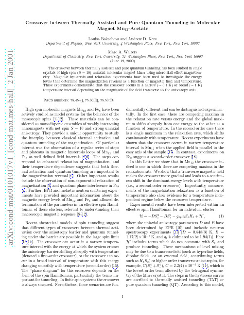
a r X i v :c o n d -m a t /0101017v 1 [c o n d -m a t .m e s -h a l l ] 2 J a n 2001Crossover between Thermally Assisted and Pure Quantum Tunneling in MolecularMagnet Mn 12-AcetateLouisa Bokacheva and Andrew D.KentDepartment of Physics,New York University,4Washington Place,New York,New York 10003Marc A.WaltersDepartment of Chemistry,New York University,31Washington Place,New York,New York 10003(June 19,2000)The crossover between thermally assisted and pure quantum tunneling has been studied in single crystals of high spin (S =10)uniaxial molecular magnet Mn 12using micro-Hall-effect magnetom-etry.Magnetic hysteresis and relaxation experiments have been used to investigate the energy levels that determine the magnetization reversal as a function of magnetic field and temperature.These experiments demonstrate that the crossover occurs in a narrow (∼0.1K)or broad (∼1K)temperature interval depending on the magnitude of the field transverse to the anisotropy axis.PACS numbers:75.45+j,75.60.Ej,75.50.TtHigh spin molecular magnets Mn 12and Fe 8have been actively studied as model systems for the behavior of the mesoscopic spins [1–12].These materials can be con-sidered as monodisperse ensembles of weakly interacting nanomagnets with net spin S =10and strong uniaxial anisotropy.They provide a unique opportunity to study the interplay between classical thermal activation and quantum tunneling of the magnetization.Of particular interest was the observation of a regular series of steps and plateaus in magnetic hysteresis loops of Mn 12and Fe 8at well defined field intervals [2,3].The steps cor-respond to enhanced relaxation of magnetization,and their temperature dependence suggests that both ther-mal activation and quantum tunneling are important to the magnetization reversal [5].Other important results include the observation of non-exponential relaxation of magnetization [3]and quantum phase interference in Fe 8[7].Further,EPR and inelastic neutron scattering exper-iments have provided important information about the magnetic energy levels of Mn 12and Fe 8and allowed de-termination of the parameters in an effective spin Hamil-tonian of these clusters,relevant to understanding their macroscopic magnetic response [8–12].Recent theoretical models of spin tunneling suggest that different types of crossovers between thermal acti-vation over the anisotropy barrier and quantum tunnel-ing under the barrier are possible in the large spin limit [13,14].The crossover can occur in a narrow tempera-ture interval with the energy at which the system crosses the anisotropy barrier shifting abruptly with temperature (denoted a first-order crossover),or the crossover can oc-cur in a broad interval of temperature with this energy changing smoothly with temperature (second-order)[15].The “phase diagram”for this crossover depends on the form of the spin Hamiltonian,particularly the terms im-portant for tunneling.In finite spin systems the crossover is always smeared.Nevertheless,these scenarios are fun-damentally different and can be distinguished experimen-tally.In the first case,there are competing maxima in the relaxation rate versus energy and the global maxi-mum shifts abruptly from one energy to the other as a function of temperature.In the second-order case there is a single maximum in the relaxation rate,which shifts continuously with temperature.Recent experiments have shown that the crossover occurs in narrow temperature interval in Mn 12when the applied field is parallel to the easy axis of the sample [17].In contrast,experiments on Fe 8suggest a second-order crossover [18].In this Letter we show that in Mn 12the crossover in-deed is one in which there are competing maxima in the relaxation rate.We show that a transverse magnetic field makes the crossover more gradual and leads to a continu-ous shift in the dominant energy levels with temperature (i.e.,a second-order crossover).Importantly,measure-ments of the magnetization relaxation as a function of temperature also show evidence for a temperature inde-pendent regime below the crossover temperature.Experimental results have been interpreted within an effective spin Hamiltonian for an individual cluster:H =−DS 2z −BS 4z −g z µB S z H z +H ′,(1)where the uniaxial anisotropy parameters D and B havebeen determined by EPR [10]and inelastic neutron spectroscopy experiments [11][D =0.548(3)K,B =1.17(2)×10−3K,and g z is estimated to be 1.94(1)].Here H ′includes terms which do not commute with S z and produce tunneling.These mechanisms of level mixing may be due to a transverse field (such as hyperfine fields,dipolar fields,or an external field,contributing terms such as H x S x )or higher order transverse anisotropies,forexample,C (S 4++S 4−),C =2.2(4)×10−5K [11],which is the lowest-order term allowed by the tetragonal symme-try of the Mn 12crystal.The steps in the hysteresis curves are ascribed to thermally assisted tunneling (TAT)or pure quantum tunneling (QT).According to this model,the magnetization relaxation occurs by tunneling from magnetic sublevels (m =10,9,8,...,−8,−9,−10),when two levels on the opposite sides of the barrier are brought close to resonance by the magnetic field.From the un-perturbed Hamiltonian (1)the longitudinal (z -axis)field at which the levels m esc and m ′become degenerate is:H (n,m esc )=nH 0{1+B/D [m 2esc +(m esc −n )2]}(2)where n =m esc +m ′is the step index describing the bias field and H 0=D/g z µB is a constant (0.42T).The transverse anisotropy does not significantly change the resonance fields,as we have checked by direct numerical diagonalization of the Hamiltonian (1).Note that larger magnetic field is necessary to bring lower lying sublevels into resonance.As the temperature decreases,the thermal population of the excited levels is reduced,and these states contribute less and less to the tunneling.Consequently,the steps in hysteresis curves shift to higher bias field values,and steps with larger n become observable.At low temperature,tunneling from the lowest level in the metastable well dominates,and the position and amplitude of the steps become indepen-dent of temperature,denoted the pure quantum tunnel-ing regime (QT).-1-0.50.51M / M sH z (Tesla)FIG.1.Hysteresis curves of a Mn 12single crystal measured at θ=35◦for three different initial magnetization states:M 0=0,0.54M s ,−M s .Inset shows the change of the n =3peak position vs magnetization at the step.Circles show data points from hysteresis measurements,squares are from field sweeps across the peak.Our experiments have been conducted using a micro-Hall-effect magnetometer [19]in a high field helium 3system.Single crystals of Mn 12in the shape of paral-lelepipeds 50×50×200µm 3were synthesized accord-ing to the procedure described in Ref.[20].The crystal was encapsulated in thermally conducting grease and the temperature was measured with a calibrated carbon ther-mometer a few millimeters from the sample.The angle θbetween the easy axis of the crystal and the applied magnetic field was varied by rotating the sample in a su-perconducting solenoid.Three different orientations have been studied:θ=0◦,20◦,and 35◦,within an accuracy of a few degrees.Hysteresis curves obtained for θ=35◦are shown on Fig. 1.The sample was prepared in three different ini-tial magnetization states:M 0=0,0.54M s ,−M s ,by field cooling,then the field was ramped at a constant rate (0.2T/min)towards positive saturation.The curves show steps and plateaus,separated by a field interval of ap-proximately 0.44T,in agreement with previously pub-lished results.The inset of Fig.1shows the field posi-tion of the n =3step versus sample magnetization at this step.The displayed data were obtained from hysteresis measurements such as those shown in Fig.1and from measurements in which the field was swept back and forth across the step,with the sample magnetization varying on each crossing.The peak positions are seen to depend slightly on the sample magnetization due to the average internal dipolar fields.Assuming that the peak positions are a linear function of magnetization,H z =B z −4παM z ,an average α,determined from different peaks,is approx-imately 0.51.A series of isothermal hysteresis measurements have been performed in small intervals of temperature,start-ing with the sample initially saturated (M =−M s ).Fig-ure 2shows a plot of the derivative of magnetization dM/dH versus the longitudinal applied field at differ-ent temperatures for two orientations,20◦and 35◦.The positions and structure of the peaks in dM/dH show the magnetic fields at which there are maxima in the magne-tization relaxation rate at a given temperature,applied field,and magnetization.The dashed lines mark the po-sitions of the experimental maxima showing their shift with temperature.Consider the data for 20◦,shown in Fig.2(a).As the temperature decreases from 1.34to 1.2K,the maximum in dM/dH (at H =1.97T)shifts to higher field values.At T =1.24K,two high-field shoul-ders appear,which can be interpreted as the “turning on”of relaxation from energy levels closer to the bottom of the potential well.Between 1.34and 1.17K,amplitude in the lower field peaks is reduced,and at T =1.17K the three peaks are of approximately equal height.However,when the temperature decreases by 0.03K,the maxi-mum shifts to the peak which occurs at H =2.16T.On lowering the temperature from 1.14to 0.94K,the amplitude of the low-field peaks decreases,which meansthat the tunneling from excited levels is “frozen out”.At T <1K only one maximum at H =2.16T survives,and its amplitude and position remain independent of tem-perature down to 0.6K,which we associate with pure QT.We can compare the positions of the peaks in this pic-ture with the values of the resonant field,calculated ac-cording to Eq.(2).The high temperature regime cor-responds to tunneling mostly from m esc =8,for which H (4,8)=1.97T.The peaks appearing at higher fields are due to tunneling from m esc =9[H (4,9)=2.06T]and m esc =10[H (4,10)=2.17T].In the pure quantum regime the ground state,m esc =10,dominates the tun-neling.The crossover from m esc =8(TAT)to m esc =10(QT)occurs over an interval of less than 0.05K.In contrast with this abrupt crossover,for θ=35◦the peak with the same index n =4shifts gradually to the higher field in the range of 1.35−0.75K,as shown on Fig.2(b).Below approximately 0.75K,the peak re-mains at a constant field value of 2.11T,which indicates the transition to the quantum regime.In this case the three escape levels,m esc =8,9,and 10are active over comparable temperature intervals,which are marked by small steps on the dashedline.d (M /M s )/d H (1/T)H z (Tesla)H z (Tesla)FIG.2.Field derivative of normalized magnetization vs H z at different temperatures for two orientations of the applied field and magnetic easy axis:a)θ=20◦,showing an abrupt crossover,andb)θ=35◦,showing a smooth crossoverto QT.Thecurves are offset forclarity.The dashed linemarks the positionof the maximumin dM/dH .Notethat the dataon graphs a)andb)are plottedon differentscales.3579B z / B 0T (K)FIG.3.Peak positions (in the units of B 0=0.42T)vs temperature for θ=0◦(squares),θ=20◦(triangles),θ=35◦(circles).The bars on the left hand side of the graph show the escape levels calculated using Eq.(2).The accuracy with which the peak positions can be determined is approximately the size of the symbol.Peak position data as a function of temperature are summarized in Fig.3,which shows the values of the longitudinal field,at which the maxima of the peaks oc-cur,versus temperature for the three studied orienta-tions.As mentioned above,determination of the peak positions must take into account the internal magnetic fields in the crystal.These depend on both the magne-tization and the crystal shape (via the demagnetization factors).We have used the correction coefficient αto determine the shift due to the magnetization of the sam-ple:B z =H z +4παM z .The maximum correction is ∆B z =8παM s =0.064T and is relatively small on the scale of the plot in Fig. 3.The bars on the left hand side of the figure show the escape levels calculated by using Eq.(2),with parameters from spectroscopic data [10,11].The correspondence between these levels and the observed peak positions is remarkably good,given the approximations involved in the analysis.By analyzing this graph,we can make following ob-servations.First,for larger angles,and therefore higher transverse field,peaks with lower indices can be observed in the experimental time window.The lowest step ob-served for θ=0◦is n =5,for θ=20◦it is n =4,for θ=35◦it is n =3.This is consistent with the idea that the transverse field promotes tunneling and lowers the effective anisotropy barrier.We find that there is greater amplitude in lower lying peaks as the transverse field is increased.Second,two regimes can be distin-guished:the high temperature regime,where the peaks gradually shift to higher fields with decreasing temper-ature,and the low temperature regime,where the peakpositions are constant.We associate the first regime with the TAT and the second with pure QT.Third,the form of the crossover between these two regimes depends on the applied field.For each sample orientation,peaks with lower indices (smaller H z )show a more abrupt crossover between TAT and QT than peaks with higher indices (compare peaks n =6and n =7for θ=0◦,or n =4and 5for θ=20◦,or n =3and 4for θ=35◦).m (t )m (t )Time (seconds)FIG.4.Relaxation of the magnetization vs time at differ-ent temperatures for a)n =6,θ=0◦,showing a crossover to a quantum regime at approximately 1K,and b)n =4,θ=35◦,showing no temperature independent regime.m (t )is a reduced magnetization:m (t )=(M s −M (t ))/2M s .In a)the five curves below 0.74K overlap (0.56K,0.58K,0.63K,0.68K,0.74K).These curves can be fit with m (t )=m 0exp((−t/τ)β),where m 0=0.94±0.01,τ=(5.45±0.15)·104s,β=0.48±0.02.The fit over-laps the data.In b)the unmarked curves from top to bottom correspond to T =0.68K,0.70K,0.75K,0.83K,0.91K,0.95K.The crossover from TAT to QT is also evident in mag-netization relaxation measurements.In these experi-ments the sample was first saturated (M =−M s ),then the field was ramped (at 0.2T/min)to a certain value and held constant for 1h,during which the magnetiza-tion was measured as a function of time.Figure 4shows two sets of relaxation curves measured at 0◦and 35◦at the fields where peaks n =6and n =4,respectively,oc-cur at the lowest temperature.For n =6,θ=0◦below approximately 1.1K,the relaxation curves are spaced very closely,i.e.,the relaxation rate almost does not change,while at higher temperature it changes signifi-cantly.This temperature corresponds to the crossover temperature seen in Fig.3–consistent with pure QT.In contrast,for the peak n =4,θ=35◦,the magneti-zation relaxation rate changes significantly as the tem-perature decreases in the entire studied range.Relax-ation curves can be fit by a stretched exponential function m (t )=m 0exp(−(t/τ)β),where β≈0.4−0.6.This form of relaxation has been observed previously in Fe 8[3]and in Mn 12[21],although it is not completely understood [22].In summary,we have presented new low temperature magnetic studies of thermally assisted and pure quan-tum tunneling in Mn 12.The crossover between these two regimes was found to be either abrupt or gradual,depending on the magnitude and orientation of applied magnetic field.Higher longitudinal and transverse fields broaden the crossover,consistent with a recent model [23].We have also shown that below the crossover tem-perature the magnetization relaxation becomes temper-ature independent.We note that the measured crossover temperature (∼1.1K)is significantly higher than pre-dicted (0.6K)[24].This may be due to an intrinsic mech-anism promoting tunneling in Mn 12such as a transverse anisotropy.Further studies of this crossover will lead to a better understanding of the mechanisms of relaxation in Mn 12.This work was supported by NSF-INT (Grant No.9513143)and NYU.[4]R.Sessoli,D.Gatteschi,A.Caneschi,and M.A.Novak,Nature365,141(1993).[5]M.Novak and R.Sessoli,in Quantum Tunneling ofMagnetization-QTM’94,ed.by L.Gunther and B.Bar-bara(Kluwer Publishing,Dordrecht,1995)p.171; B.Barbara et al.,JMMM140-144,1825(1995).[6]J.M.Hernandez et al.,Europhys.Lett.35,301(1996).[7]W.Wernsdorfer and R.Sessoli,Science284,133(1999).[8]S.Hill et al.,Phys.Rev.Lett.80,2453(1998).[9]M.Hennion et al.,Phys.Rev.B56,8819(1997).[10]A.L.Barra,D.Gatteschi,and R.Sessoli,Phys.Rev.B56,8192(1997).[11]I.Mirebeau et al.,Phys.Rev.Lett.83,628(1999).[12]Y.Zhong et al.,J.Appl.Phys.85,5636(1999).[13]E.M.Chudnovsky and D.A.Garanin,Phys.Rev.Lett.79,4469(1997).[14]G.-H.Kim,Phys.Rev.B59,11847(1999);G.-H.Kim,Europhys.Lett.51,216(2000);H.J.W.M¨u ller-Kirsten,D.K.Park,and J.M.S.Rana,Phys.Rev.B60,6662(1999),and references therein.[15]The analogy to phase transitions is a purely formal oneas discussed in[13].Thefirst-order,second-order termi-nology for the escape rate crossover is originally due to Larkin and Ovchinnikov[16].[16]rkin and Y.N.Ovchinnikov,Sov.Phys.JETP59,420(1984).[17]A.D.Kent et al.,Europhys.Lett.49,512(2000).[18]W.Wernsdorfer et al.,Europhys.Lett.50,552(2000).[19]A. D.Kent,S.von Molnar,S.Gider,and D. D.Awschalom,J.Appl.Phys.76,6656(1994).[20]T.Lis,Acta Cryst.B36,2042(1980).[21]L.Tomas,A.Caneschi,and B.Barbara,Phys.Rev.Lett.83,2398(1999).[22]N.V.Prokof’ev and P.C.E.Stamp,Phys.Rev.Lett.80,5794(1998); E.M.Chudnovsky,Phys.Rev.Lett.84,5676(2000);N.V Prokof’ev and P. C. E.Stamp, ibid.,84,5677(2000);W.Wernsdorfer,C.Paulsen,and R.Sessoli,ibid.,84,5678(2000).[23]D.A.Garanin,X.Hidalgo,and E.M.Chudnovsky,Phys.Rev.B57,13639(1998).[24]L.Bokacheva,A.D.Kent,and M.A.Walters,Polyhe-dron(to be published).。

Ornstein–Uhlenbeck process - Wikipedia,the f...Ornstein–Uhlenbeck process undefinedundefinedFrom Wikipedia, the free encyclopediaJump to: navigation, searchNot to be confused with Ornstein–Uhlenbeck operator.In mathematics, the Ornstein–Uhlenbeck process (named after LeonardOrnstein and George Eugene Uhlenbeck), is a stochastic process that, roughly speaking, describes the velocity of a massive Brownian particle under the influence of friction. The process is stationary, Gaussian, and Markov, and is the only nontrivial process that satisfies these three conditions, up to allowing linear transformations of the space and time variables.[1] Over time, the process tends to drift towards its long-term mean: such a process is called mean-reverting.The process x t satisfies the following stochastic differential equation:where θ> 0, μ and σ> 0 are parameters and W t denotes the Wiener process. Contents[hide]1 Application in physical sciences2 Application in financialmathematics3 Mathematical properties4 Solution5 Alternative representation6 Scaling limit interpretation7 Fokker–Planck equationrepresentation8 Generalizations9 See also10 References11 External links[edit] Application in physical sciencesThe Ornstein–Uhlenbeck process is a prototype of a noisy relaxation process. Consider for example a Hookean spring with spring constant k whose dynamics is highly overdamped with friction coefficient γ. In the presence of thermal fluctuations with temperature T, the length x(t) of the spring will fluctuate stochastically around the spring rest length x0; its stochastic dynamic is described by an Ornstein–Uhlenbeck process with:where σ is derived from the Stokes-Einstein equation D = σ2 / 2 = k B T / γ for theeffective diffusion constant.In physical sciences, the stochastic differential equation of an Ornstein–Uhlenbeck process is rewritten as a Langevin equationwhere ξ(t) is white Gaussian noise with .At equilibrium, the spring stores an averageenergy in accordance with the equipartition theorem.[edit] Application in financial mathematicsThe Ornstein–Uhlenbeck process is one of several approaches used to model (with modifications) interest rates, currency exchange rates, and commodity prices stochastically. The parameter μ represents the equilibrium or mean value supported by fundamentals; σ the degree of volatility around it caused by shocks, and θ the rate by which these shocks dissipate and the variable reverts towards the mean. One application of the process is a trading strategy pairs trade.[2][3][edit] Mathematical propertiesThe Ornstein–Uhlenbeck process is an example of a Gaussian process that has a bounded variance and admits a stationary probability distribution, in contrast tothe Wiener process; the difference between the two is in their "drift" term. For the Wiener process the drift term is constant, whereas for the Ornstein–Uhlenbeck process it is dependent on the current value of the process: if the current value of the process is less than the (long-term) mean, the drift will be positive; if the current valueof the process is greater than the (long-term) mean, the drift will be negative. In other words, the mean acts as an equilibrium level for the process. This gives the process its informative name, "mean-reverting." The stationary (long-term) variance is given byThe Ornstein–Uhlenbeck process is the continuous-time analogue ofthe discrete-time AR(1) process.three sample paths of different OU-processes with θ = 1, μ = 1.2, σ = 0.3:blue: initial value a = 0 (a.s.)green: initial value a = 2 (a.s.)red: initial value normally distributed so that the process has invariant measure [edit] SolutionThis equation is solved by variation of parameters. Apply Itō–Doeblin's formula to thefunctionto getIntegrating from 0 to t we getwhereupon we seeThus, the first moment is given by (assuming that x0 is a constant)We can use the Itōisometry to calculate the covariance function byThus if s < t (so that min(s, t) = s), then we have[edit] Alternative representationIt is also possible (and often convenient) to represent x t (unconditionally, i.e.as ) as a scaled time-transformed Wiener process:or conditionally (given x0) asThe time integral of this process can be used to generate noise with a 1/ƒpower spectrum.[edit] Scaling limit interpretationThe Ornstein–Uhlenbeck process can be interpreted as a scaling limit of a discrete process, in the same way that Brownian motion is a scaling limit of random walks. Consider an urn containing n blue and yellow balls. At each step a ball is chosen at random and replaced by a ball of the opposite colour. Let X n be the number of blueballs in the urn after n steps. Then converges to a Ornstein–Uhlenbeck process as n tends to infinity.[edit] Fokker–Planck equation representationThe probability density function ƒ(x, t) of the Ornstein–Uhlenbeck process satisfies the Fokker–Planck equationThe stationary solution of this equation is a Gaussian distribution with mean μ and variance σ2 / (2θ)[edit ] GeneralizationsIt is possible to extend the OU processes to processes where the background driving process is a L évy process . These processes are widely studied by OleBarndorff-Nielsen and Neil Shephard and others.In addition, processes are used in finance where the volatility increases for larger values of X . In particular, the CKLS (Chan-Karolyi-Longstaff-Sanders) process [4] with the volatility term replaced by can be solved in closed form for γ = 1 / 2 or 1, as well as for γ = 0, which corresponds to the conventional OU process.[edit ] See alsoThe Vasicek model of interest rates is an example of an Ornstein –Uhlenbeck process.Short rate model – contains more examples.This article includes a list of references , but its sources remain unclear because it has insufficient inline citations .Please help to improve this article by introducing more precise citations where appropriate . (January 2011)[edit ] References^ Doob 1942^ Advantages of Pair Trading: Market Neutrality^ An Ornstein-Uhlenbeck Framework for Pairs Trading ^ Chan et al. (1992)G.E.Uhlenbeck and L.S.Ornstein: "On the theory of Brownian Motion", Phys.Rev.36:823–41, 1930. doi:10.1103/PhysRev.36.823D.T.Gillespie: "Exact numerical simulation of the Ornstein–Uhlenbeck process and its integral", Phys.Rev.E 54:2084–91, 1996. PMID9965289doi:10.1103/PhysRevE.54.2084H. Risken: "The Fokker–Planck Equation: Method of Solution and Applications", Springer-Verlag, New York, 1989E. Bibbona, G. Panfilo and P. Tavella: "The Ornstein-Uhlenbeck process as a model of a low pass filtered white noise", Metrologia 45:S117-S126,2008 doi:10.1088/0026-1394/45/6/S17Chan. K. C., Karolyi, G. A., Longstaff, F. A. & Sanders, A. B.: "An empirical comparison of alternative models of the short-term interest rate", Journal of Finance 52:1209–27, 1992.Doob, J.L. (1942), "The Brownian movement and stochastic equations", Ann. of Math.43: 351–369.[edit] External linksA Stochastic Processes Toolkit for Risk Management, Damiano Brigo, Antonio Dalessandro, Matthias Neugebauer and Fares TrikiSimulating and Calibrating the Ornstein–Uhlenbeck process, M.A. van den Berg Calibrating the Ornstein-Uhlenbeck model, M.A. van den BergMaximum likelihood estimation of mean reverting processes, Jose Carlos Garcia FrancoRetrieved from ""。

专业词汇列表晶体结构（structure of crystal）原子质量单位 Atomic mass unit (amu)原子量 Atomic weight键能 Bonding energy共价键 Covalent bond电子构型 electronic configuration正电的 Electropositive氢键 Hydrogen bond同位素 Isotope摩尔 Mole泡利不相容原理 Pauli exclusion principle原子 atom分子量 molecule weight量子数 quantum number范德华键 van der waals bond点群 point group各向异性 anisotropy体心立方结构 body-centered cubic (BCC)布拉格定律bragg’s law晶体结构 crystal structure晶体的 crystalline中子衍射 neutron diffraction晶界 grain boundary鲍林规则Pauling’s rulesCsCl型结构 Caesium Chloride structure纤锌矿型结构 Wurtzite structure萤石型结构 Fluorite structure尖晶石型结构 Spinel-type structure岛状结构 Island structure层状结构 Layer structure滑石 talc高岭石 kaolinite长石 feldspar各向同性的 isotropic晶格 lattice密勒指数 miller indices多晶的 polycrystalline原子数 Atomic number波尔原子模型 Bohr atomic model库仑力 Coulombic force分子的构型 molecular configuration负电的 Electronegative基态 Ground state离子键 Ionic bond金属键Metallic bond分子 Molecule元素周期表 Periodic table极性分子 Polar molecule价电子 valence electron电子轨道 electron orbitals对称要素 symmetry elements原子堆积因数 atomic packing factor(APF)面心立方结构 face-centered cubic (FCC)配位数 coordination number晶系 crystal system衍射 diffraction电子衍射 electron diffraction六方密堆积 hexagonal close-packed (HCP)NaCl型结构 NaCl－type structure闪锌矿型结构 Blende-type structure金红石型结构 Rutile structure钙钛矿型结构 Perovskite-type structure硅酸盐结构 Structure of silicates链状结构 Chain structure架状结构 Framework structure叶蜡石 pyrophyllite石英 quartz美橄榄石 forsterite各向异性的 anisotropy晶格参数 lattice parameters非结晶的 noncrystalline多晶形 polymorphism单晶 single crystal电位 electron states电子 electrons金属键 metallic bonding极性分子 polar molecules衍射角 diffraction angle粒度,晶粒大小 grain size显微照相 photomicrograph透射电子显微镜 transmission electron microscope (TEM)四方的 tetragonal配位数 coordination number晶胞 unit cell(化合)价 valence共价键 covalent bonding离子键 Ionic bonding原子面密度 atomic planar density合金 alloy显微结构 microstructure扫描电子显微镜 scanning electron microscope (SEM)重量百分数weight percent单斜的monoclinic晶体结构缺陷(defect of crystal structure)缺陷 defect, imperfection线缺陷 line defect, dislocation体缺陷 volume defect位错线 dislocation line螺位错 screw dislocation晶界 grain boundaries小角度晶界 tilt boundary,位错阵列 dislocation array位错轴 dislocation axis位错爬移 dislocation climb位错滑移 dislocation slip位错裂纹 dislocation crack位错密度 dislocation density间隙原子 interstitial atom间隙位置 interstitial sites弗伦克尔缺陷 Frenkel disorder主晶相 the host lattice缔合中心 Associated Centers.电子空穴 Electron Holes克罗各-明克符号 Kroger Vink notation固溶体 solid solution化合物 compound置换固溶体 substitutional solid solution不混溶固溶体 immiscible solid solution有序固溶体 ordered solid solution固溶强化 solid solution strengthening点缺陷 point defect面缺陷 interface defect位错排列 dislocation arrangement刃位错 edge dislocation混合位错 mixed dislocation大角度晶界 high-angle grain boundaries孪晶界 twin boundaries位错气团 dislocation atmosphere位错胞 dislocation cell位错聚结 dislocation coalescence位错核心能量 dislocation core energy位错阻尼 dislocation damping原子错位 substitution of a wrong atom晶格空位 vacant lattice sites杂质 impurities肖脱基缺陷 Schottky disorder错位原子 misplaced atoms自由电子 Free Electrons伯格斯矢量 Burgers中性原子 neutral atom固溶度 solid solubility间隙固溶体 interstitial solid solution金属间化合物 intermetallics转熔型固溶体 peritectic solid solution无序固溶体 disordered solid solution取代型固溶体 Substitutional solid solutions过饱和固溶体 supersaturated solid solution非化学计量化合物 Nonstoichiometric compound表面结构与性质(structure and property of surface)表面 surface同相界面 homophase boundary晶界 grain boundary小角度晶界 low angle grain boundary共格孪晶界 coherent twin boundary错配度 mismatch重构 reconstuction表面能 surface energy扭转晶界 twist grain boundary共格界面 coherent boundary非共格界面 noncoherent boundary应变能 strain energy惯习面 habit plane界面 interface异相界面 heterophase boundary表面能 surface energy大角度晶界 high angle grain boundary晶界迁移 grain boundary migration驰豫 relaxation表面吸附 surface adsorption倾转晶界 titlt grain boundary倒易密度 reciprocal density半共格界面 semi-coherent boundary界面能 interfacial free energy晶体学取向关系 crystallographic orientation非晶态结构与性质(structure and property of uncrystalline) 熔体结构 structure of melt玻璃态 vitreous state粘度 viscosity介稳态过渡相 metastable phase淬火 quenching玻璃分相 phase separation in glasses 过冷液体 supercooling melt软化温度 softening temperature表面张力 Surface tension组织 constitution退火的 softened体积收缩 volume shrinkage扩散(diffusion)活化能 activation energy浓度梯度 concentration gradient菲克第二定律Fick’s second law稳态扩散 steady state diffusion扩散系数 diffusion coefficient填隙机制 interstitalcy mechanism短路扩散 short-circuit diffusion下坡扩散 Downhill diffusion扩散通量 diffusion flux菲克第一定律Fick’s first law相关因子 correlation factor非稳态扩散 nonsteady-state diffusion 跳动几率 jump frequency晶界扩散 grain boundary diffusion上坡扩散 uphill diffusion互扩散系数 Mutual diffusion渗碳剂 carburizing浓度分布曲线 concentration profile 驱动力 driving force自扩散 self-diffusion空位扩散 vacancy diffusion扩散方程 diffusion equation扩散特性 diffusion property达肯方程 Dark equation本征热缺陷 Intrinsic thermal defect 离子电导率 Ion-conductivity浓度梯度 concentration gradient扩散流量 diffusion flux间隙扩散 interstitial diffusion表面扩散 surface diffusion扩散偶 diffusion couple扩散机理 diffusion mechanism无规行走 Random walk柯肯达尔效应 Kirkendall equation本征扩散系数 Intrinsic diffusion coefficient 空位机制 Vacancy concentration腐蚀与氧化（corroding and oxidation）氧化反应 Oxidation reaction还原反应 Reduction reaction价电子 Valence electron腐蚀介质 Corroding solution电动势 Electric potential推动力 The driving force腐蚀系统 Corroding system腐蚀速度 Corrosion penetration rate电流密度 Current density电化学反应 Electrochemical reaction极化作用 Polarization过电位 The over voltage浓差极化 Concentration polarization电化学极化 Activation polarization极化曲线 Polarization curve缓蚀剂 Inhibitor原电池 galvanic cell电偶腐蚀 galvanic corrosion电位序 galvanic series应力腐蚀 Stress corrosion冲蚀 Erosion-corrosion腐蚀短裂 Corrosion cracking防腐剂 Corrosion remover腐蚀电极 Corrosion target隙间腐蚀 Crevice corrosion均匀腐蚀 Uniform attack晶间腐蚀 Intergranular corrosion焊缝破坏 Weld decay选择性析出 Selective leaching氢脆损坏 Hydrogen embitterment阴极保护 Catholic protection穿晶断裂 Intergranular fracture固相反应和烧结(solid state reaction and sintering) 固相反应 solid state reaction烧成 fire再结晶 Recrystallization成核 nucleation子晶，雏晶 matted crystal异质核化 heterogeneous nucleation铁碳合金 iron-carbon alloy铁素体 ferrite共晶反应 eutectic reaction烧结 sintering合金 alloy二次再结晶 Secondary recrystallization结晶 crystallization耔晶取向 seed orientation均匀化热处理 homogenization heat treatment渗碳体 cementite奥氏体 austenite固溶处理 solution heat treatment相变 (phase transformation)过冷 supercooling晶核 nucleus形核功 nucleation energy均匀形核 homogeneous nucleation形核率 nucleation rate热力学函数 thermodynamics function临界晶核 critical nucleus枝晶偏析 dendritic segregation平衡分配系数 equilibrium distribution coefficient成分过冷 constitutional supercooling共晶组织 eutectic structure伪共晶 pseudoeutectic表面等轴晶区 chill zone中心等轴晶区 equiaxed crystal zone急冷技术 splatcooling单晶提拉法 Czochralski method位错形核 dislocation nucleation斯宾那多分解 spinodal decomposition马氏体相变 martensite phase transformation成核机理 nucleation mechanism过冷度 degree of supercooling形核 nucleation晶体长大 crystal growth非均匀形核 heterogeneous nucleation长大速率 growth rate临界晶核半径 critical nucleus radius局部平衡 localized equilibrium有效分配系数 effective distribution coefficient 引领（领先）相 leading phase层状共晶体 lamellar eutectic离异共晶 divorsed eutectic柱状晶区 columnar zone定向凝固 unidirectional solidification区域提纯 zone refining晶界形核 boundary nucleation晶核长大 nuclei growth有序无序转变 disordered-order transition马氏体 martensite成核势垒 nucleation barrier相平衡与相图（Phase equilibrium and Phase diagrams）相图 phase diagrams组分 component相律 Phase rule浓度三角形 Concentration triangle成分 composition相平衡 phase equilibrium热力学 thermodynamics吉布斯相律 Gibbs phase rule吉布斯自由能 Gibbs free energy吉布斯熵 Gibbs entropy热力学函数 thermodynamics function过冷 supercooling杠杆定律 lever rule相界线 phase boundary line共轭线 conjugate lines相界反应 phase boundary reaction相组成 phase composition金相相组织 phase constentuent相衬显微镜 phase contrast microscope 相分布 phase distribution相平衡图 phase equilibrium diagram 相分离 phase segregation相 phase组元 compoonent投影图 Projection drawing冷却曲线 Cooling curve自由度 freedom化学势 chemical potential相律 phase rule自由能 free energy吉布斯混合能 Gibbs energy of mixing 吉布斯函数 Gibbs function热分析 thermal analysis过冷度 degree of supercooling相界 phase boundary相界交联 phase boundary crosslinking相界有限交联 phase boundary crosslinking 相变 phase change共格相 phase-coherent相衬 phase contrast相衬显微术 phase contrast microscopy相平衡常数 phase equilibrium constant相变滞后 phase transition lag相序 phase order相稳定性 phase stability相稳定区 phase stabile range相变压力 phase transition pressure同素异晶转变 allotropic transformation 显微结构 microstructures不混溶性 immiscibility相态 phase state相变温度 phase transition temperature同质多晶转变 polymorphic transformation 相平衡条件 phase equilibrium conditions。

Abbreviation --> 缩写词 About --> 关于 absolut --> 绝对 Active --> 当前add --> 增加 add/edit/delete --> 增加 / 编辑 /删除 Additional Out --> 附加输出 adius --> 心Adjacent --> 相邻 Adv --> 高级 Advection --> 对流 Algorithm --> 算法 align --> 定位Align WP with --> 工作区排列按 ALPX --> 热膨胀系数 Also 副词 再Ambient Condit'n --> 环境条件 amplitude --> 振幅 Analysis --> 分析 Angle --> 角度 Angles --> 角度 Angular --> 角度 Animate --> 动画 Animation --> 动画 Anno --> 注释Anno/Graph --> 注释 / 图 Annotation --> 注释文字 Annulus --> 环面ANSYSMultiphysics Utility Menu --> ANSYS 综合物理场有限元分析 菜单Any --> 任意apply --> 应用Arbitrary --> 任意 arccosine --> 反余弦Archive --> 合并Arcs --> 圆弧线 arcsine --> 反正弦 area --> 面Area Fillet --> 面圆角 Area Mesh --> 已划分的面 Areas --> 面 Array --> 数组 arrow --> 箭头 Assembly --> 部件At Coincid Nd --> 在两节点间 Attch 动词 接触 Attr --> 特征Attrib --> 属性 Attributes --> 属性 Auto --> 自动Automatic Fit --> 自适应 Axes --> 坐标轴 Axis --> 坐标轴Axi-Symmetric --> 轴对称 back up --> 恢复Background --> 背景 Banded --> 条状 Based --> 基础 BC --> 边界Beam --> 梁 behavior --> 特性 Bellows --> ［密封 ］波纹管 Bias --> 偏置Biot Savart --> 毕奥 -萨瓦河 Bitmap --> BMP 图片 Block --> 块 Body --> 体Booleans --> 布尔操作 box --> 框 Branch --> 分支brick orient --> 划分块 ( 方向 ) Builder --> 生成器 Built-up --> 合成Buoyancy Terms --> 浮力项By Circumscr Rad --> 外切正多边形By End KPs -->始点、终点 By End Points --> 直径圆 By End Pts --> 底圆直径By Inscribed Rad --> 内接 ?正多边 形By Picking --> 鼠标选取By Side Length --> 通过边长确定 多边形By Vertices --> 通过顶点确定多边形calc --> 运算 Calcs --> 计算 Capacitor --> 电容Capped/Q-Slice --> 切面透明度设置Capping --> 盖 Capture --> 打印Cartesian --> 笛卡儿坐标系 Case --> 情况CE Node Selected --> 约束节点选择cent 中心 Center --> 中心 centr 中心 ceqn --> 约束CFD --> 计 算 流 体 力 学 (CFD) Change 动词 更换 Check --> 检查 Checking --> 检查 Checks --> 检查 Circle --> 圆Circuit --> 电路 circumscr --> 外接圆 Clr Size --> 清除尺寸 CMS --> 组件模式综合 Cnst --> 常数 Cntl --> 控制 Cntrls --> 控制 Coincident --> 重合 Collapse --> 折叠收起 Color --> 颜色 Colors --> 颜色 Common --> 普通 Comp --> 组件complex variable --> 复数变量 Component --> 组件 Components --> 组件 Compress --> 精减 Concats --> 未划分Concentrate --> 集中 concrete --> 混凝土Cond --> 导体 Conditions --> 条件 cone --> 圆锥 Configuration --> 配置 Connectivity --> 连通性Connt --> 连通区域 consistent --> 固定 Const --> 常数Constant Amplitude --> 恒幅 Constants --> 常数 Constr --> 约束 Constraint --> 约束Constraints --> 约束 constreqn --> 约束方程 Contact --> 接触 Contour --> 等值线Abbreviation --> 缩写词 About --> 关于 absolut --> 绝对 Active --> 当前Contour Plot --> 等值云图 Contours --> 等值线 contraction --> 收缩因子Database --> 数据库DB --> DB definitns --> 特征定义 Deformed --> 已变形Degen --> 退化 Degeneracy --> 退化 Control --> 控制 Controls --> 控制 CONVERGENCEINDICATOR --> 收 敛精度CONVERGENCE VALUE --收> 敛值 Convert ALPx -->热膨胀系数转换 Coor --> 坐标系 Coord --> 坐标Coord Sys --> 坐标系 coordinate --> 坐标 Coordinates --> 坐标 Coords --> 坐标 corner --> 对角 Corners --> 对角 cornr --> 对角 correl field --> 相关性区域 correlation --> 相关性 count --> 总数 Couple --> 耦合 Coupled --> 耦合 Coupling --> 耦合 CP NodeSelected --> 耦合节点选择 Create 动词 新建 creep --> 蠕变 criteria --> 准则 cross product --> 向量积 cross-sectional --> 截面 CS --> 坐标系 csys --> 坐标系 ctr --> 中点 ctrl --> 控制 ctrls --> 控制 Cupl --> 耦合 Curr --> 电流 curvature --> 圆弧 Curvature Ctr --> 曲率中心 Curve --> 曲线 custom --> 定制 Cyc --> 循环Cyclic Expansion -->循环扩展设置 Cyclic Model --> 周向模型 Cyclic Sector --> 扇型周向阵列 cylinder --> 圆柱Cylindrical --> 柱坐标系 Damper --> 阻尼 ［减震 ］器 damping --> 阻尼系数 Data --> 数据Data Tables --> 数据表格 Del --> 删除Del Concats --> 删除连接 Delete --> 删除 dependent --> 相关 derivative --> 导数Design Opt --> 优化设计 Device --> 设备 differentiate --> 微分 Digitize --> 数字化 dimensions --> 尺寸 Diode --> 二极管 Directory --> 目录 discipline --> 练习 Displacement --> 变形 Display --> 显示 distances --> 距离 Divide --> 划分 Divs --> 位置DOF --> 自由度 dofs --> 自由度 dot product --> 点积 Dupl --> 复制 edge --> 边缘 Edit --> 编辑Elbow --> 弯管 ［肘管 ］ ElecMech --> 电磁 ElecStruc --> 静电 -结构 electr --> 电磁Electric --> 电气类 electromag --> 电磁 electromagnetic --> 电磁 Electromechanic --> 电 -机械 elem --> 单元Elem Birth/Death --> 单元生 / 死 Element --> 单元Elements --> 单元 Elems --> 单元 Elm --> 单元 EMT CDISP -->电磁陷阱CDISP Enable 形容词允许 ENDS --> 端 energy --> 能量 ENKE --> 湍动能量Entities --> 实体 Entity --> 实体 EPPL COMP -->塑性应变分量 EPTO COMP -->总应变 eq --> 方程Eqn --> 方程 Eqns --> 方程 equation --> 方程式Erase --> 删除 Est. --> 估算 Everything --> 所有 EX --> 弹性模量EX exclude --> 排除 Execute --> 执行 Execution --> 执行 Expansion --> 扩展 Expend All --> 展开全部 Exponential --> 幂数 ［指数］ exponentiate --> 幂指数 Export --> 模型输出 Ext Opts --> 拉伸设置 Extend Line --> 延伸线 extra --> 附加 extreme --> 极值 Extrude --> 拉伸 EY --> 弹性模量EY EZ -->弹性模量 EZ face --> 面 Facets --> 表面粗糙 fact --> 因子 factor --> 系数 factr --> 因子 failure --> 破坏 Fast Sol'n --> 快速求解 Fatigue --> 疲劳 FD --> 失效挠度 field --> 区域 Fill --> 填充Fill between KPs -->关键点间填入 Fill between Nds --> 节点间填充 fillet --> 倒角Fit --> 适当视图 Flange --> 法兰 Flip --> 翻转Floating Point --> 浮点 FLOTRAN --> 流体FLOTRAN Set Up -->流体运行设置 Flow --> 流量kps --> 关键点 Labeling --> 标志 Layer --> 层Layered --> 分层 Layers --> 层 Fluid --> 流体 Flux --> 通量 Fnc_/EXI --> 退出Fnc_/GRAPHICS -->图形界面 Focus Point --> 焦点 force --> 力 Format --> 格式 Fourier --> 傅立叶级数Free --> 自由 Freq --> 频率 From Full --> 完全 Full Circle --> 完整圆 Func --> 函数 function --> 函数 Functions --> 函数 Gap --> 间隙 Gen --> 一般 General --> 通用 General Options --> 通用设置 General Postproc-->通用后处理器 Generator --> 生成器Genl --> 普通 Geom --> 单元 Geometry --> 几何形状Get --> 获取 Global --> 全局 Globals --> 全局 Glue --> 粘合 gradient --> 梯度 Graph --> 图Graphics --> 图形 Graphs --> 图 Gravity --> 引力 （ 重力 ） Grid --> 网格 GUI --> 图形用户界面 GXY --> 剪切模量GXY GXZ -->剪切模量 GXZ GYZ -->剪切模量 GYZ hard --> 硬 Hard Points --> 硬点 Hard PT --> 硬点 hardening --> 强化 hex --> 六面体 Hexagon --> 六边形 Hexagonal --> 六棱柱 hidden --> 隐藏 higher-order --> 高阶 Hill --> 希尔h-method --> 网格细分法 hollow --> 空心Hollow Cylinder --> 空心圆柱体 Hollow Sphere --> 空心球体 hp-method --> 混合并行法 I-J --> I-J imaginary --> 虚部 Immediate --> 即时 Import --> 模型输入 Improve --> 改进 independent --> 非相关 Individual --> 单个 Indp Curr Src --> 感应电流源 Indp Vltg Src --> 感应电压源 Inductor --> 电感 Inertia --> 惯性 Inertia Relief Summ --> 惯量概要Inf Acoustic --> 无穷声学单元 init --> 初始化Init Condit'n --> 初始条件 Initial --> 初始 inquire --> 查询 inscribed --> 内切圆 Installation --> 安装 int --> 强度 integral --> 积分 integrat --> 积分 integrate --> 积分 interactive --> 交互式 Interface --> 接触面 intermed --> 中间 interpolate --> 插入 Intersect --> 相交 invert --> 切换 is done --> 完成 Isometric --> 等轴侧视图 Isosurfaces --> 常值表面 isotropic --> 各向同性 Item --> 项目 Items --> 项目Iteration --> 叠代 Jobname --> 文件名Joint --> 连接 Joints --> 连接 KABS --> KABS Keypoint --关> 键点 Keypoints --> 关键点 kinematic --> 随动 KP --> 关键点KP between KPs -->关键点间设置 Layout --> 布局 Lay-up --> 层布置 Ld --> 载荷Legal Notices --> 法律声明 Legend --> 图例 Lib --> 库文件 Library --> 材料库文件 Licensing --> 许可 Light Source --> 光源设置 line --> 线 Line Fillet --> 圆角 Line Mesh --> 已划分的线 Line w/Ratio --> 线上 / 比例 Linear --> 线性 Linearized --> 线形化 Lines --> 线 List --> 列出 List Results --> 列表结果 Ln' s --> 段 Load --> 加载 Load Step --> 载荷步 Loads --> 载荷 Loc --> 坐标值Local --> 局部 Locate --> 定位 Location --> 位置 Locations --> 位置 Locs --> 位置Log File --> 命令流记录文件 lower-order --> 低阶LSDYNA --> LSDYN/动力分析） LS-DYNA --> 显示动力分析 Macro --> 宏命令 Magnification --> 放大倍数 management --> 管理 Manager --> 管理器 manual --> 手动 ManualSize --> 手动尺寸 Map --> 图 Mapped --> 映射 Mass --> 导体Mass Type --> 聚合量类型 Master --> 主pretension --> 主张 Pretensn --> 自划分 prism --> 棱柱Pro --> Pro Prob --> 概率 profiles --> 档案资料mat --> 材料 Mat Num --> 材料编号 Material --> 材料 Materials --> 材料 matl --> 材料 Matls --> 材料 maximum --> 最大 Mechanical --> 机械类 member --> 构件 memory --> 内存 MenuCtrls --> 菜单控制 Merge --> 合并 mesh --> 网格 Mesher --> 网格 Meshing --> 网格划分 MeshTool --> 网格工具 Message --> 消息 Metafile --> 图元文件 Meth --> 方法MIR --> 修正惯性松弛 Miter --> 斜接 [管 ] Mod --> 更改 Mode --> 模式 Model --> 模型 Modeling --> 建模 Models --> 模型 Modify --> 修改 Modle --> 模型 Module --> 模块 moment --> 力矩More --> 更多 multi --> 多 multi-field --> 多物理场耦合 Multilegend --> 多图 multilinear --> 多线性 Multiple Species --> 多倍样式 multiplied --> 乘 Multi-Plot --> 多窗口绘图Multi-Plots --> 多图表 Multi-Window --> 多窗口Mutual Ind --> 互感 Name --> 名称 Named --> 已指定 natural log --> 自然对数 nd --> 节点 nds --> 节点NL Generalized -->非线形普通梁截面No Expansion --> 不扩展 Nodal --> 节点 Node --> 节点 Nonlin --> 非线性 Nonlinear --> 非线性Non-uniform --> 不均匀 norm --> 法向Normal --> 法向 Normals --> 没 Num --> 编号NUMB --> NUMB Number --> 编号 Numbered --> 编号 Numbering --> 编号 Numbers --> 编号 NUXY --> 泊松比 Oblique --> 等角轴侧视图 Octagon --> 八边形Octagonal --> 八棱柱 offset --> 偏移Offset WP by Increments --> 指针 增量偏移Offset WP to --> 指针偏移到 Operate --> 操作 Operations --> 运算 OPT --> 优化 Options --> 设置 Optn --> 设置 opts --> 设置 Ord --> 指令 Order --> 顺序 Orders --> 指令Orient Normals --> 确定最外层法 向 Origin --> 原点Orthotropic --> 正交各向异性 Other --> 其他Out Derived --> 输出派生 outp --> 输出 Output --> 输出Over Results --> 整个过程结果 Over Time --> 规定时间内全过程 Overlaid --> 覆盖 Overlap --> 重叠 Pair --> 偶Pairwise --> 新生成的 Pan --> 移动pan-zoom-rotate --> 移动 -缩放 -旋转par --> 参数名 parall --> 平行 Parameters --> 参数 Parms --> 参数 Part IDs --> 部分 ID 号 Partial --> 部分Partial Cylinder --> 部分圆柱体 Particle Flow --> 粒子流迹 Partition --> 分割 Parts --> 局部 Path --> 路径PDS --> 概率设计系统Pentagon --> 五边形 Pentagonal --> 五棱柱Percent Error --> 误差率Periodic/Cyclic Symmetry--> 周 期 / 循环 阵列Perspective --> 透视 phase --> 相位 pick --> 选取 Picked --> 已选取Piecewise --> 分段 Piezoelectric --> 压电元件 Pipe --> 管 Pipe Run --> 管操作 Pipe Tee --> T 型管 Piping --> 管 Plane --> 平面Plane Strn --> 平面应变 plasticity --> 塑性 plot --> 绘图 plotctrls --> 绘图控制 Plots --> 绘图P-method --> 高次单元法 Pointer --> 指针 poisson --> 泊松 Polygon --> 多边形 POST1 --> 通用后处理器 POST26 --> 时间历程后处理器 postpro --> 后处理器 postproc --> 后处理器 potential --> 势POWRGRPH -->激活窗体 preferences --> 参数选项 Pre-integrated --> 前集成处理 PREP7 --> 前处理器 preprocessor --> 前处理器PRES --> 压力Pre-tens Elements --> 删除单元后 合并节点Prop --> 属性Properties --> 属性Props --> 属性PRXY -->泊松比PRXY PRXZ -->泊松比PRXZ PRYZ -->泊松比PRYZ PT -->点Pts --> 点Pulse --> 脉冲Q-Slice --> 切面Quad --> 积分Quadratic --> 二次qualities --> 质量query --> 查询QUIT --> 退出R --> 圆rad --> 半径radiation --> 辐射矩阵radius --> 半径Raise --> 升起random --> 随机range of variable --> 变量范围rate --> 率Rate of Change for ModelMainpulation --> 模型缩放变化率设定Reaction --> 反作用Read --> 读取Read Input from --> 读取命令流文件Real Constante --> 实常数RealConst --> 实常数Rectangle --> 矩形Redirect --> 重定向Reducer --> 接头ref --> 判定Refine --> 细化Reflect --> 阵列reflection --> 镜像Region --> 区域Regions --> 区域Relax/Stab/Cap --> 松弛/稳定/ 容量Relaxation --> 松弛release --> 版本Remesh --> 重划网格remove --> 删除rename --> 重命名Reorder --> 重置Replay Animation --> 重新播放动画Replot --> 重新绘图Report --> 报告Report --> 报告Res/Quad --> 结果/ 积分Reselect --> 分解Reset --> 取消Residual --> 余量Resistor --> 电阻response --> 响应Restart --> 重启动Restart/Clear --> 重启动/ 清除Restart/Iteration --> 重启动/ 迭代Restart/Load step --> 重启动/ 载荷步Restart/Set --> 重启动/ 设置Restart/Time --> 重启动/ 时间片Restore --> 恢复Result --> 结果Results --> 结果RESUM --> 恢复RESUM_DB --> 恢复_DB resume --> 恢复Reverse --> 相反Reverse Video --> 反色图像Rigid --> 刚性ROM --> 存储器Rotary --> 扭转Rotate --> 旋转Rotating --> 旋转rotational --> 旋转RUNSTAR -->估计分析模块SAT --> SAT SAVE --保> 存SAVE_DB -->保存_DBScalar --> 变量scale --> 比例scale factor --> 比例因子Scale Icon --> 图符尺度Scaling --> 比例Screen --> 屏幕se --> 超级单元secn --> 截面号sect --> 截面Sect Mesh --> 自定义网格Section --> 截面Sections --> 截面Sector --> 部分Segment --> 分段SegmentMemory --> 分段保存segmented--> 分段Segments --> 分段Sel --> 选择sele --> 选择Select--> 选择Selected --> 已选择Selection --> 选择septagon -->七边形septagonal --> 七边形的Set --> 设置Set Grid --> 设置栅格Set Up --> 设置Sets --> 设置Settings --> 设置Shaded -->阴影Shape --> 形状Shell -->壳Show --> 显示sided --> 边sine --> 正弦Singularity --> 奇异点sint --> 应力强度Sinusoidal --> 正弦Size --> 尺寸skinning --> 2 线Slide Film --> 滑动薄膜Smart --> 精确SmartSize --> 智能尺寸Solid --> 实体Solid Circle --> 定圆心圆SolidCylinder --> 定圆心圆柱体SolidSphere --> 定圆心球体Solu -->求解SOLUTION --> 求解器Solver --> 求解Sort --> 排序source --> 源Specification --> 约定Specifications --> 明细单Specified --> 指定Specified --> 指定Specified Loc --> 指定局部坐标spectrm --> 响应谱Spectrum --> 频谱pretension --> 主张 Pretensn --> 自划分 prism --> 棱柱 Pro --> Pro Prob --> 概率 profiles --> 档案资料Sphere --> 球体 Spherical --> 球坐标系 spline --> 样条Splines --> 样条曲线 SpotWeld --> 点焊 [缝、接点 ] Spring --> 弹簧Spring Support --> 弹性支撑 Spring-Gap Supp -->弹性间隙支撑 Src Waveform --> 屏幕波形 Standed --> 标准 Start --> 开始 Start New --> 新建 Start Num --> 初始编号Start Number --> 初始编号 state --> 状态 stats --> 状态 Status --> 状态 step --> 步 store --> 存贮 stress --> 应力 Stresses --> 应力 strn --> 应变 Strnd Coil --> 线圈struct --> 结构 structural --> 结构 Style --> 样式 submodeling --> 子模型Subtract --> 减去Summary --> 概要 superelem --> 超单元 superelement --> 超单元 Superelements --> 超单元 surf --> 表面Surface --> 面 Surfaces --> 表面Sweep --> 扫描 switch --> 转换 Symbols --> 符号Symmetry Expansion --> 模型对称 性扩展 -镜像复制扫描 Sys --> 系统Table --> 表 tan --> 相切 tangent --> 相切 Taper --> 锥形 Target --> 目标 tech --> 技术 TEMP --> 温度Temp Variatio --> 临时变量 Temps --> 温度 Tet --> 四面体 Tets --> 测试 Textured --> 纹理 Texturing --> 材质thermal --> 热Thickness --> 壳厚度 thickness func --> 函数定义变化 的厚度 Through --> 通过 thru --> 通过Time Integration --> 时间积分 Time Stepping --> 时间步设定 Time-harmonic --> 时间 -谐波 timehist --> 时间历程TimeHist Postproc --> 时间历程后 处理器 Title --> 标题 Toggle --> 扭转 Tolerance --> 误差 T oolbar --> 工具栏 Topics --> 主题 topological --> 拓扑 torus --> 环行圆柱 Trace --> 痕迹 Trans --> 传递 Transducer --> 传感器 Transducers --> 传感器 Transfer --> 移动 Transient --> 暂态Translucency --> 半透视设置 Traveling Wave --> 传导波 Triangle --> 三角形 Triangular --> 三棱柱 ttribs --> 属性 Turbulence --> 湍流 Tutorials --> 指南 Type --> 类型 Types --> 类型 Uniform --> 均布 Units --> 单位 Unload --> 卸载 unpick --> 排除 Unselect --> 不选择 Update --> 更新 user --> 用户User Numbered --> 自定义编号 User Specified Expansion --> 自定 义扩展模式utility --> 应用分析 value --> 值Valve --> 阀 Variables --> 变量 Vector --> 矢量 vectors --> 矢量Vector-Scalar --> 矢量 -变量 VFRC --> 体积含量 View --> 视图 Viewing --> 视图 visco --> 粘 Vltg --> 电压 VOF --> 流体 Volm --> 体 Volms --> 体Volu --> 体 volume --> 体 Volumes --> 立体Volumes Brick Orient --> 沿 Z 向立 方体 Volus --> 体 VS --> 电压源 VX -->速度X 方向VY --> 速度 Y 方向 VZ --> 速度 Z 方向 w/Same --> w/ 相同节点 Warning/Error --> 警告 /错误 warp --> 翘曲Wavefront --> 波前 win --> 窗口 Window --> 窗口 Wire --> 导线 wish --> 希望 with --> 通过 Working --> 工作 Working Plane --> 工作平面 WorkPlane --> 工作平面 WP --> 工作平面WP Status --> 工作区指针状态 Write DB log file --> 写入日志 WrkPlane --> 工作面Zener --> 齐纳 Zoom --> 缩放。

a r X i v :g r -q c /0411082v 1 16 N o v 2004Laser Ranging to the Moon,Mars and BeyondSlava G.Turyshev,James G.Williams,Michael Shao,John D.AndersonJet Propulsion Laboratory,California Institute of Technology,4800Oak Grove Drive,Pasadena,CA 91109,USAKenneth L.Nordtvedt,Jr.Northwest Analysis,118Sourdough Ridge Road,Bozeman,MT 59715USA Thomas W.Murphy,Jr.Physics Department,University of California,San Diego 9500Gilman Dr.,La Jolla,CA 92093USA Abstract Current and future optical technologies will aid exploration of the Moon and Mars while advancing fundamental physics research in the solar system.Technologies and possible improvements in the laser-enabled tests of various physical phenomena are considered along with a space architecture that could be the cornerstone for robotic and human exploration of the solar system.In particular,accurate ranging to the Moon and Mars would not only lead to construction of a new space communication infrastructure enabling an improved navigational accuracy,but will also provide a significant improvement in several tests of gravitational theory:the equivalence principle,geodetic precession,PPN parameters βand γ,and possible variation of the gravitational constant G .Other tests would become possible with an optical architecture that would allow proceeding from meter to centimeter to millimeter range accuracies on interplanetary distances.This paper discusses the current state and the future improvements in the tests of relativistic gravity with Lunar Laser Ranging (LLR).We also consider precision gravitational tests with the future laser rangingto Mars and discuss optical design of the proposed Laser Astrometric Test of Relativity (LATOR)mission.We emphasize that already existing capabilities can offer significant improvements not only in the tests of fundamental physics,but may also establish the infrastructure for space exploration in the near future.Looking to future exploration,what characteristics are desired for the next generation of ranging devices,what is the optimal architecture that would benefit both space exploration and fundamental physics,and what fundamental questions can be investigated?We try to answer these questions.1IntroductionThe recent progress in fundamental physics research was enabled by significant advancements in many technological areas with one of the examples being the continuing development of the NASA Deep Space Network –critical infrastructure for precision navigation and communication in space.A demonstration of such a progress is the recent Cassini solar conjunction experiment[8,6]that was possible only because of the use of Ka-band(∼33.4GHz)spacecraft radio-tracking capabilities.The experiment was part of the ancillary science program–a by-product of this new radio-tracking technology.Becasue of a much higher data rate transmission and, thus,larger data volume delivered from large distances the higher communication frequency was a very important mission capability.The higher frequencies are also less affected by the dispersion in the solar plasma,thus allowing a more extensive coverage,when depp space navigation is concerned.There is still a possibility of moving to even higher radio-frequencies, say to∼60GHz,however,this would put us closer to the limit that the Earth’s atmosphere imposes on signal transmission.Beyond these frequencies radio communication with distant spacecraft will be inefficient.The next step is switching to optical communication.Lasers—with their spatial coherence,narrow spectral emission,high power,and well-defined spatial modes—are highly useful for many space applications.While in free-space,optical laser communication(lasercomm)would have an advantage as opposed to the conventional radio-communication sercomm would provide not only significantly higher data rates(on the order of a few Gbps),it would also allow a more precise navigation and attitude control.The latter is of great importance for manned missions in accord the“Moon,Mars and Beyond”Space Exploration Initiative.In fact,precision navigation,attitude control,landing,resource location, 3-dimensional imaging,surface scanning,formationflying and many other areas are thought only in terms of laser-enabled technologies.Here we investigate how a near-future free-space optical communication architecture might benefit progress in gravitational and fundamental physics experiments performed in the solar system.This paper focuses on current and future optical technologies and methods that will advance fundamental physics research in the context of solar system exploration.There are many activities that focused on the design on an optical transceiver system which will work at the distance comparable to that between the Earth and Mars,and test it on the Moon.This paper summarizes required capabilities for such a system.In particular,we discuss how accurate laser ranging to the neighboring celestial bodies,the Moon and Mars,would not only lead to construction of a new space communication infrastructure with much improved navigational accuracy,it will also provide a significant improvement in several tests of gravitational theory. Looking to future exploration,we address the characteristics that are desired for the next generation of ranging devices;we will focus on optimal architecture that would benefit both space exploration and fundamental physics,and discuss the questions of critical importance that can be investigated.This paper is organized as follows:Section2discusses the current state and future per-formance expected with the LLR technology.Section3addresses the possibility of improving tests of gravitational theories with laser ranging to Mars.Section4addresses the next logical step—interplanetary laser ranging.We discuss the mission proposal for the Laser Astrometric Test of Relativity(LATOR).We present a design for its optical receiver system.Section5 addresses a proposal for new multi-purpose space architecture based on optical communica-tion.We present a preliminary design and discuss implications of this new proposal for tests of fundamental physics.We close with a summary and recommendations.2LLR Contribution to Fundamental PhysicsDuring more than35years of its existence lunar laser ranging has become a critical technique available for precision tests of gravitational theory.The20th century progress in three seem-ingly unrelated areas of human exploration–quantum optics,astronomy,and human spaceexploration,led to the construction of this unique interplanetary instrument to conduct very precise tests of fundamental physics.In this section we will discuss the current state in LLR tests of relativistic gravity and explore what could be possible in the near future.2.1Motivation for Precision Tests of GravityThe nature of gravity is fundamental to our understanding of the structure and evolution of the universe.This importance motivates various precision tests of gravity both in laboratories and in space.Most of the experimental underpinning for theoretical gravitation has come from experiments conducted in the solar system.Einstein’s general theory of relativity(GR)began its empirical success in1915by explaining the anomalous perihelion precession of Mercury’s orbit,using no adjustable theoretical parameters.Eddington’s observations of the gravitational deflection of light during a solar eclipse in1919confirmed the doubling of the deflection angles predicted by GR as compared to Newtonian and Equivalence Principle(EP)arguments.Follow-ing these beginnings,the general theory of relativity has been verified at ever-higher accuracy. Thus,microwave ranging to the Viking landers on Mars yielded an accuracy of∼0.2%from the gravitational time-delay tests of GR[48,44,49,50].Recent spacecraft and planetary mi-crowave radar observations reached an accuracy of∼0.15%[4,5].The astrometric observations of the deflection of quasar positions with respect to the Sun performed with Very-Long Base-line Interferometry(VLBI)improved the accuracy of the tests of gravity to∼0.045%[45,51]. Lunar Laser Ranging(LLR),the continuing legacy of the Apollo program,has provided ver-ification of GR improving an accuracy to∼0.011%via precision measurements of the lunar orbit[62,63,30,31,32,35,24,36,4,68].The recent time-delay experiments with the Cassini spacecraft at a solar conjunction have tested gravity to a remarkable accuracy of0.0023%[8] in measuring deflection of microwaves by solar gravity.Thus,almost ninety years after general relativity was born,Einstein’s theory has survived every test.This rare longevity and the absence of any adjustable parameters,does not mean that this theory is absolutely correct,but it serves to motivate more sensitive tests searching for its expected violation.The solar conjunction experiments with the Cassini spacecraft have dramatically improved the accuracy in the solar system tests of GR[8].The reported accuracy of2.3×10−5in measuring the Eddington parameterγ,opens a new realm for gravitational tests,especially those motivated by the on-going progress in scalar-tensor theories of gravity.1 In particular,scalar-tensor extensions of gravity that are consistent with present cosmological models[15,16,17,18,19,20,39]predict deviations of this parameter from its GR value of unity at levels of10−5to10−7.Furthermore,the continuing inability to unify gravity with the other forces indicates that GR should be violated at some level.The Cassini result together with these theoretical predictions motivate new searches for possible GR violations;they also provide a robust theoretical paradigm and constructive guidance for experiments that would push beyond the present experimental accuracy for parameterized post-Newtonian(PPN)parameters(for details on the PPN formalism see[60]).Thus,in addition to experiments that probe the GR prediction for the curvature of the gravityfield(given by parameterγ),any experiment pushingthe accuracy in measuring the degree of non-linearity of gravity superposition(given by anotherEddington parameterβ)will also be of great interest.This is a powerful motive for tests ofgravitational physics phenomena at improved accuracies.Analyses of laser ranges to the Moon have provided increasingly stringent limits on anyviolation of the Equivalence Principle(EP);they also enabled very accurate measurements fora number of relativistic gravity parameters.2.2LLR History and Scientific BackgroundLLR has a distinguished history[24,9]dating back to the placement of a retroreflector array onthe lunar surface by the Apollo11astronauts.Additional reflectors were left by the Apollo14and Apollo15astronauts,and two French-built reflector arrays were placed on the Moon by theSoviet Luna17and Luna21missions.Figure1shows the weighted RMS residual for each year.Early accuracies using the McDonald Observatory’s2.7m telescope hovered around25cm. Equipment improvements decreased the ranging uncertainty to∼15cm later in the1970s.In1985the2.7m ranging system was replaced with the McDonald Laser Ranging System(MLRS).In the1980s ranges were also received from Haleakala Observatory on the island of Maui in theHawaiian chain and the Observatoire de la Cote d’Azur(OCA)in France.Haleakala ceasedoperations in1990.A sequence of technical improvements decreased the range uncertainty tothe current∼2cm.The2.7m telescope had a greater light gathering capability than thenewer smaller aperture systems,but the newer systemsfired more frequently and had a muchimproved range accuracy.The new systems do not distinguish returning photons against thebright background near full Moon,which the2.7m telescope could do,though there are somemodern eclipse observations.The lasers currently used in the ranging operate at10Hz,with a pulse width of about200 psec;each pulse contains∼1018photons.Under favorable observing conditions a single reflectedphoton is detected once every few seconds.For data processing,the ranges represented by thereturned photons are statistically combined into normal points,each normal point comprisingup to∼100photons.There are15553normal points are collected until March2004.Themeasured round-trip travel times∆t are two way,but in this paper equivalent ranges in lengthunits are c∆t/2.The conversion between time and length(for distance,residuals,and dataaccuracy)uses1nsec=15cm.The ranges of the early1970s had accuracies of approximately25cm.By1976the accuracies of the ranges had improved to about15cm.Accuracies improvedfurther in the mid-1980s;by1987they were4cm,and the present accuracies are∼2cm.One immediate result of lunar ranging was the great improvement in the accuracy of the lunarephemeris[62]and lunar science[67].LLR measures the range from an observatory on the Earth to a retroreflector on the Moon. For the Earth and Moon orbiting the Sun,the scale of relativistic effects is set by the ratio(GM/rc2)≃v2/c2∼10−8.The center-to-center distance of the Moon from the Earth,with mean value385,000km,is variable due to such things as eccentricity,the attraction of the Sun,planets,and the Earth’s bulge,and relativistic corrections.In addition to the lunar orbit,therange from an observatory on the Earth to a retroreflector on the Moon depends on the positionin space of the ranging observatory and the targeted lunar retroreflector.Thus,orientation ofthe rotation axes and the rotation angles of both bodies are important with tidal distortions,plate motion,and relativistic transformations also coming into play.To extract the gravitationalphysics information of interest it is necessary to accurately model a variety of effects[68].For a general review of LLR see[24].A comprehensive paper on tests of gravitationalphysics is[62].A recent test of the EP is in[4]and other GR tests are in[64].An overviewFigure1:Historical accuracy of LLR data from1970to2004.of the LLR gravitational physics tests is given by Nordtvedt[37].Reviews of various tests of relativity,including the contribution by LLR,are given in[58,60].Our recent paper describes the model improvements needed to achieve mm-level accuracy for LLR[66].The most recent LLR results are given in[68].2.3Tests of Relativistic Gravity with LLRLLR offers very accurate laser ranging(weighted rms currently∼2cm or∼5×10−11in frac-tional accuracy)to retroreflectors on the Moon.Analysis of these very precise data contributes to many areas of fundamental and gravitational physics.Thus,these high-precision studies of the Earth-Moon-Sun system provide the most sensitive tests of several key properties of weak-field gravity,including Einstein’s Strong Equivalence Principle(SEP)on which general relativity rests(in fact,LLR is the only current test of the SEP).LLR data yielded the strongest limits to date on variability of the gravitational constant(the way gravity is affected by the expansion of the universe),and the best measurement of the de Sitter precession rate.In this Section we discuss these tests in more details.2.3.1Tests of the Equivalence PrincipleThe Equivalence Principle,the exact correspondence of gravitational and inertial masses,is a central assumption of general relativity and a unique feature of gravitation.EP tests can therefore be viewed in two contexts:tests of the foundations of general relativity,or as searches for new physics.As emphasized by Damour[12,13],almost all extensions to the standard modelof particle physics(with best known extension offered by string theory)generically predict newforces that would show up as apparent violations of the EP.The weak form the EP(the WEP)states that the gravitational properties of strong and electro-weak interactions obey the EP.In this case the relevant test-body differences are their fractional nuclear-binding differences,their neutron-to-proton ratios,their atomic charges,etc. General relativity,as well as other metric theories of gravity,predict that the WEP is exact. However,extensions of the Standard Model of Particle Physics that contain new macroscopic-range quantumfields predict quantum exchange forces that will generically violate the WEP because they couple to generalized‘charges’rather than to mass/energy as does gravity[17,18]. WEP tests can be conducted with laboratory or astronomical bodies,because the relevant differences are in the test-body compositions.Easily the most precise tests of the EP are made by simply comparing the free fall accelerations,a1and a2,of different test bodies.For the case when the self-gravity of the test bodies is negligible and for a uniform external gravityfield, with the bodies at the same distance from the source of the gravity,the expression for the Equivalence Principle takes the most elegant form:∆a= M G M I 2(1)(a1+a2)where M G and M I represent gravitational and inertial masses of each body.The sensitivity of the EP test is determined by the precision of the differential acceleration measurement divided by the degree to which the test bodies differ(position).The strong form of the EP(the SEP)extends the principle to cover the gravitational properties of gravitational energy itself.In other words it is an assumption about the way that gravity begets gravity,i.e.about the non-linear property of gravitation.Although general relativity assumes that the SEP is exact,alternate metric theories of gravity such as those involving scalarfields,and other extensions of gravity theory,typically violate the SEP[30,31, 32,35].For the SEP case,the relevant test body differences are the fractional contributions to their masses by gravitational self-energy.Because of the extreme weakness of gravity,SEP test bodies that differ significantly must have astronomical sizes.Currently the Earth-Moon-Sun system provides the best arena for testing the SEP.The development of the parameterized post-Newtonian formalism[31,56,57],allows one to describe within the common framework the motion of celestial bodies in external gravitational fields within a wide class of metric theories of gravity.Over the last35years,the PPN formalism has become a useful framework for testing the SEP for extended bodies.In that formalism,the ratio of passive gravitational to inertial mass to thefirst order is given by[30,31]:M GMc2 ,(2) whereηis the SEP violation parameter(discussed below),M is the mass of a body and E is its gravitational binding or self-energy:E2Mc2 V B d3x d3yρB(x)ρB(y)EMc2 E=−4.64×10−10andwhere the subscripts E and m denote the Earth and Moon,respectively.The relatively small size bodies used in the laboratory experiments possess a negligible amount of gravitational self-energy and therefore such experiments indicate nothing about the equality of gravitational self-energy contributions to the inertial and passive gravitational masses of the bodies [30].TotesttheSEP onemustutilize planet-sizedextendedbodiesinwhichcase theratioEq.(3)is considerably higher.Dynamics of the three-body Sun-Earth-Moon system in the solar system barycentric inertial frame was used to search for the effect of a possible violation of the Equivalence Principle.In this frame,the quasi-Newtonian acceleration of the Moon (m )with respect to the Earth (E ),a =a m −a E ,is calculated to be:a =−µ∗rM I m µS r SEr 3Sm + M G M I m µS r SEr 3+µS r SEr 3Sm +η E Mc 2 m µS r SEMc 2 E − E n 2−(n −n ′)2n ′2a ′cos[(n −n ′)t +D 0].(8)Here,n denotes the sidereal mean motion of the Moon around the Earth,n ′the sidereal mean motion of the Earth around the Sun,and a ′denotes the radius of the orbit of the Earth around the Sun (assumed circular).The argument D =(n −n ′)t +D 0with near synodic period is the mean longitude of the Moon minus the mean longitude of the Sun and is zero at new Moon.(For a more precise derivation of the lunar range perturbation due to the SEP violation acceleration term in Eq.(6)consult [62].)Any anomalous radial perturbation will be proportional to cos D .Expressed in terms ofη,the radial perturbation in Eq.(8)isδr∼13ηcos D meters [38,21,22].This effect,generalized to all similar three body situations,the“SEP-polarization effect.”LLR investigates the SEP by looking for a displacement of the lunar orbit along the direction to the Sun.The equivalence principle can be split into two parts:the weak equivalence principle tests the sensitivity to composition and the strong equivalence principle checks the dependence on mass.There are laboratory investigations of the weak equivalence principle(at University of Washington)which are about as accurate as LLR[7,1].LLR is the dominant test of the strong equivalence principle.The most accurate test of the SEP violation effect is presently provided by LLR[61,48,23],and also in[24,62,63,4].Recent analysis of LLR data test the EP of∆(M G/M I)EP=(−1.0±1.4)×10−13[68].This result corresponds to a test of the SEP of∆(M G/M I)SEP=(−2.0±2.0)×10−13with the SEP violation parameter η=4β−γ−3found to beη=(4.4±4.5)×10−ing the recent Cassini result for the PPN parameterγ,PPN parameterβis determined at the level ofβ−1=(1.2±1.1)×10−4.2.3.2Other Tests of Gravity with LLRLLR data yielded the strongest limits to date on variability of the gravitational constant(the way gravity is affected by the expansion of the universe),the best measurement of the de Sitter precession rate,and is relied upon to generate accurate astronomical ephemerides.The possibility of a time variation of the gravitational constant,G,wasfirst considered by Dirac in1938on the basis of his large number hypothesis,and later developed by Brans and Dicke in their theory of gravitation(for more details consult[59,60]).Variation might be related to the expansion of the Universe,in which case˙G/G=σH0,where H0is the Hubble constant, andσis a dimensionless parameter whose value depends on both the gravitational constant and the cosmological model considered.Revival of interest in Brans-Dicke-like theories,with a variable G,was partially motivated by the appearance of superstring theories where G is considered to be a dynamical quantity[26].Two limits on a change of G come from LLR and planetary ranging.This is the second most important gravitational physics result that LLR provides.GR does not predict a changing G,but some other theories do,thus testing for this effect is important.The current LLR ˙G/G=(4±9)×10−13yr−1is the most accurate limit published[68].The˙G/G uncertaintyis83times smaller than the inverse age of the universe,t0=13.4Gyr with the value for Hubble constant H0=72km/sec/Mpc from the WMAP data[52].The uncertainty for˙G/G is improving rapidly because its sensitivity depends on the square of the data span.This fact puts LLR,with its more then35years of history,in a clear advantage as opposed to other experiments.LLR has also provided the only accurate determination of the geodetic precession.Ref.[68]reports a test of geodetic precession,which expressed as a relative deviation from GR,is K gp=−0.0019±0.0064.The GP-B satellite should provide improved accuracy over this value, if that mission is successfully completed.LLR also has the capability of determining PPNβandγdirectly from the point-mass orbit perturbations.A future possibility is detection of the solar J2from LLR data combined with the planetary ranging data.Also possible are dark matter tests,looking for any departure from the inverse square law of gravity,and checking for a variation of the speed of light.The accurate LLR data has been able to quickly eliminate several suggested alterations of physical laws.The precisely measured lunar motion is a reality that any proposed laws of attraction and motion must satisfy.The above investigations are important to gravitational physics.The future LLR data will improve the above investigations.Thus,future LLR data of current accuracy would con-tinue to shrink the uncertainty of˙G because of the quadratic dependence on data span.The equivalence principle results would improve more slowly.To make a big improvement in the equivalence principle uncertainty requires improved range accuracy,and that is the motivation for constructing the APOLLO ranging facility in New Mexico.2.4Future LLR Data and APOLLO facilityIt is essential that acquisition of the new LLR data will continue in the future.Accuracies∼2cm are now achieved,and further very useful improvement is expected.Inclusion of improved data into LLR analyses would allow a correspondingly more precise determination of the gravitational physics parameters under study.LLR has remained a viable experiment with fresh results over35years because the data accuracies have improved by an order of magnitude(see Figure1).There are prospects for future LLR station that would provide another order of magnitude improvement.The Apache Point Observatory Lunar Laser-ranging Operation(APOLLO)is a new LLR effort designed to achieve mm range precision and corresponding order-of-magnitude gains in measurements of fundamental physics parameters.For thefirst time in the LLR history,using a3.5m telescope the APOLLO facility will push LLR into a new regime of multiple photon returns with each pulse,enabling millimeter range precision to be achieved[29,66].The anticipated mm-level range accuracy,expected from APOLLO,has a potential to test the EP with a sensitivity approaching10−14.This accuracy would yield sensitivity for parameterβat the level of∼5×10−5and measurements of the relative change in the gravitational constant,˙G/G, would be∼0.1%the inverse age of the universe.The overwhelming advantage APOLLO has over current LLR operations is a3.5m astro-nomical quality telescope at a good site.The site in southern New Mexico offers high altitude (2780m)and very good atmospheric“seeing”and image quality,with a median image resolu-tion of1.1arcseconds.Both the image sharpness and large aperture conspire to deliver more photons onto the lunar retroreflector and receive more of the photons returning from the re-flectors,pared to current operations that receive,on average,fewer than0.01 photons per pulse,APOLLO should be well into the multi-photon regime,with perhaps5–10 return photons per pulse.With this signal rate,APOLLO will be efficient atfinding and track-ing the lunar return,yielding hundreds of times more photons in an observation than current√operations deliver.In addition to the significant reduction in statistical error(useful).These new reflectors on the Moon(and later on Mars)can offer significant navigational accuracy for many space vehicles on their approach to the lunar surface or during theirflight around the Moon,but they also will contribute significantly to fundamental physics research.The future of lunar ranging might take two forms,namely passive retroreflectors and active transponders.The advantages of new installations of passive retroreflector arrays are their long life and simplicity.The disadvantages are the weak returned signal and the spread of the reflected pulse arising from lunar librations(apparent changes in orientation of up to10 degrees).Insofar as the photon timing error budget is dominated by the libration-induced pulse spread—as is the case in modern lunar ranging—the laser and timing system parameters do√not influence the net measurement uncertainty,which simply scales as1/3Laser Ranging to MarsThere are three different experiments that can be done with accurate ranges to Mars:a test of the SEP(similar to LLR),a solar conjunction experiment measuring the deflection of light in the solar gravity,similar to the Cassini experiment,and a search for temporal variation in the gravitational constant G.The Earth-Mars-Sun-Jupiter system allows for a sensitive test of the SEP which is qualitatively different from that provided by LLR[3].Furthermore,the outcome of these ranging experiments has the potential to improve the values of the two relativistic parameters—a combination of PPN parametersη(via test of SEP)and a direct observation of the PPN parameterγ(via Shapiro time delay or solar conjunction experiments).(This is quite different compared to LLR,as the small variation of Shapiro time delay prohibits very accurate independent determination of the parameterγ).The Earth-Mars range would also provide for a very accurate test of˙G/G.This section qualitatively addresses the near-term possibility of laser ranging to Mars and addresses the above three effects.3.1Planetary Test of the SEP with Ranging to MarsEarth-Mars ranging data can provide a useful estimate of the SEP parameterηgiven by Eq.(7). It was demonstrated in[3]that if future Mars missions provide ranging measurements with an accuracy ofσcentimeters,after ten years of ranging the expected accuracy for the SEP parameterηmay be of orderσ×10−6.These ranging measurements will also provide the most accurate determination of the mass of Jupiter,independent of the SEP effect test.It has been observed previously that a measurement of the Sun’s gravitational to inertial mass ratio can be performed using the Sun-Jupiter-Mars or Sun-Jupiter-Earth system[33,47,3]. The question we would like to answer here is how accurately can we do the SEP test given the accurate ranging to Mars?We emphasize that the Sun-Mars-Earth-Jupiter system,though governed basically by the same equations of motion as Sun-Earth-Moon system,is significantly different physically.For a given value of SEP parameterηthe polarization effects on the Earth and Mars orbits are almost two orders of magnitude larger than on the lunar orbit.Below we examine the SEP effect on the Earth-Mars range,which has been measured as part of the Mariner9and Viking missions with ranging accuracy∼7m[48,44,41,43].The main motivation for our analysis is the near-future Mars missions that should yield ranging data, accurate to∼1cm.This accuracy would bring additional capabilities for the precision tests of fundamental and gravitational physics.3.1.1Analytical Background for a Planetary SEP TestThe dynamics of the four-body Sun-Mars-Earth-Jupiter system in the Solar system barycentric inertial frame were considered.The quasi-Newtonian acceleration of the Earth(E)with respect to the Sun(S),a SE=a E−a S,is straightforwardly calculated to be:a SE=−µ∗SE·r SE MI Eb=M,Jµb r bS r3bE + M G M I E b=M,Jµb r bS。