chap16 STATA编程基础

Stata软件基本操作和数据分析入门(完整版讲义)Stata软件基本操作和数据分析入门第一讲Stata操作入门张文彤赵耐青第一节概况Stata最初由美国计算机资源中心（Computer Resource Center）研制，现在为Stata公司的产品，其最新版本为7.0版。

它操作灵活、简单、易学易用，是一个非常有特色的统计分析软件，现在已越来越受到人们的重视和欢迎，并且和SAS、SPSS一起，被称为新的三大权威统计软件。

Stata最为突出的特点是短小精悍、功能强大，其最新的7.0版整个系统只有10M左右，但已经包含了全部的统计分析、数据管理和绘图等功能，尤其是他的统计分析功能极为全面，比起1G以上大小的SAS 系统也毫不逊色。

另外，由于Stata在分析时是将数据全部读入内存，在计算全部完成后才和磁盘交换数据，因此运算速度极快。

由于Stata的用户群始终定位于专业统计分析人员，因此他的操作方式也别具一格，在Windows席卷天下的时代，他一直坚持使用命令行／程序操作方式，拒不推出菜单操作系统。

但是，Stata的命令语句极为简洁明快，而且在统计分析命令的设置上又非常有条理，它将相同类型的统计模型均归在同一个命令族下，而不同命令族又可以使用相同功能的选项，这使得用户学习时极易上手。

更为令人叹服的是，Stata 语句在简洁的同时又拥有着极高的灵活性，用户可以充分发挥自己的聪明才智，熟练应用各种技巧，真正做到随心所欲。

除了操作方式简洁外，Stata的用户接口在其他方面也做得非常简洁，数据格式简单，分析结果输出简洁明快，易于阅读，这一切都使得Stata成为非常适合于进行统计教学的统计软件。

Stata的另一个特点是他的许多高级统计模块均是编程人员用其宏语言写成的程序文件（ADO文件），这些文件可以自行修改、添加和下载。

用户可随时到Stata网站寻找并下载最新的升级文件。

事实上，Stata 的这一特点使得他始终处于统计分析方法发展的最前沿，用户几乎总是能很快找到最新统计算法的Stata 程序版本，而这也使得Stata自身成了几大统计软件中升级最多、最频繁的一个。

Stata及数据处理目录第一章STATA基础 (3)1.1 命令格式 (4)1.2 缩写、关系式和错误信息 (6)1.3 do文件 (6)1.4 标量和矩阵 (7)1.5 使用Stata命令的结果 (8)1.6 宏 (10)1.7 循环语句 (11)1.8 用户写的程序 (15)1.9 参考文献 (15)1.10 练习 (15)第二章数据管理和画图 (18)2.1数据类型和格式 (18)2.2 数据输入 (19)2.3 画图 (21)第3章线性回归基础 (22)3.1 数据和数据描述 (22)3.1.1 变量描述 (23)3.1.2 简单统计 (23)3.1.3 二维表 (23)3.1.4 加统计信息的一维表 (26)3.1.5 统计检验 (26)3.1.6 数据画图 (27)3.2 回归分析 (28)3.2.1 相关分析 (28)3.2.2 线性回归 (29)3.2.3 假设检验 Wald test (30)3.2.4 估计结果呈现 (30)3.3 预测 (34)3.4 Stata 资源 (35)第4章数据处理的组织方法 (36)1、可执行程序的编写与执行 (36)方法1：do文件 (36)方法2：交互式-program-命令 (36)方法3：在do文件中使用program命令 (38)方法4：do文件合并 (39)方法5：ado 文件 (40)2、do文件的组织 (40)3、数据导入 (40)4、_n和_N的用法 (44)第一章STATA基础STATA的使用有两种方式，即菜单驱动和命令驱动。

菜单驱动比较适合于初学者，容易入学，而命令驱动更有效率，适合于高级用户。

我们主要着眼于经验分析，因而重点介绍命令驱动模式。

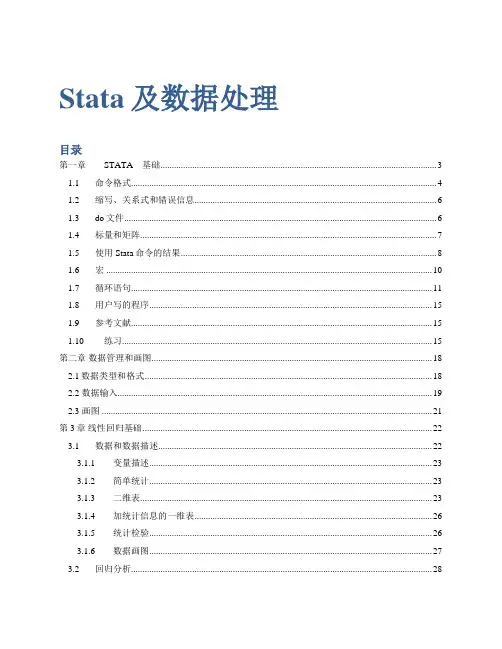
图1.1Stata12.1的基本界面关于STATA的使用，可以参考Stata手册，特别是[GS] Getting Started with Stata，尤其是第１章A sample session和第２章The Stata User Interface。

Austin Nichols***********************@austnncholsOne Weird TrickHow to analyze experiments•The only way to be sure we are estimating unbiased causal impacts ofa “treatment” (intervention, policy, program) is to compare means via anexperiment (Freedman 2018a,b, Lin 2013)•But we can always do better by conditioning on observable (pre-treatment) characteristics: these “covariates” can reduce MSE–Stratification/blocking preferred to post hoc statistical adjustment but has its own limitations (Kallus 2018)–How should one adjust for covariates if using a regression to analyze the experimental data? What variables should be included?❖Use the LASSO! Specifically, poregress, dsregress, xporegress, etc.•New to Stata as of Stata 16, explained in the new [LASSO] manual and in Drukker(2019)Partialing out• A series of seminal papers by Belloni, Chernozhukov, and many others (see references) derived partialing-out estimators that provide reliable inference for d after one uses covariate selection to determine which of many covariates “belong” in the model for outcome YY = A d + X g + ewhere A is a treatment variable of interest and X measures the (possibly verylarge) set of potential covariates, but many elements of g are zero •Essentially, run separate LASSO regressions of Y and A on X and regress residualizedŸon residualizedÄ (where Ä = A –Â )•The cost of using these poregress, dsregress, xporegress methods is that they do not produce estimates for the covariate coefficients gStata 16 LASSO manual page 12Add’l Stata implementations•ssc desc lassopack, ssc desc pdslasso(Ahrens, Hansen, and Schaffer 2018) released prior to Stata 16 implementations–They implement the LASSO (Tibshirani1996) and the square-root-lasso (Belloni et al. 2011, 2014).–These estimators can be used to select controls (pdslasso) or instruments (ivlasso) from a large set of variables (possibly numbering more than thenumber of observations), in a setting where the researcher is interested inestimating the causal impact of one or more (possibly endogenous) causal variables of interest.–Two approaches are implemented in pdslasso and ivlasso: (1) The "post-double-selection" (PDS) methodology of Belloni et al. (2012, 2013, 2014,2015, 2016). (2) The "post-regularization" (CHS) methodology ofChernozhukov, Hansen and Spindler (2015). For instrumental variableestimation, ivlasso implements weak-identification-robust hypothesis tests and confidence sets using the Chernozhukov et al. (2013) sup-score test.Regression for experiments•Note that in the model for outcome YY = A d + X g + e•We really should never care about the “effect” of any element of X conditional on A and other elements of X, i.e. we should not care one whit about estimates of g•In expectation, A and X are uncorrelated; we just want a data-driven way to eliminate chance correlation between X and A for any X that also has effects on Y in order to reduce the variance of our estimates of d•These and other points arose in email correspondence in 2016-2017 with David Judkins who has used LASSO in subsequent studies (Judkins 2019)Okay, LASSO, but what kind?•Chetverikov, Liao, and Chernozhukov(2019) show “the cross-validated LASSO estimator achieves the fastest possible rate of convergence in the prediction norm up toa small logarithmic factor”•Drukker(2019) suggests the plug-in estimator has better small-sample performance in simulations (not reported)• A bootstrap could give out-of-sample performance measures akin to RandomForest regressionsSimulations•Suppose we have hundreds of candidate regressors, all distributed lognormal, all uncorrelated with each other• A few are correlated with Y (every 20th)•How big an improvement might we expect with the xporegress cross-fit partialing-out lasso linear regression with plug-in optimal lambda?Typical Simulation Results 10,000 iterationswith N=100Regressions use allavailable controls,zero to 80+Horizontal linesshow performanceof xporegress withCV or plug-inselection optionsConclusions•As we add useless regressors, MSE increases and the occasional useful regressor does not (necessarily) make up for that, but xporegress does better in every realistic case examined •Alternatives in e.g.Judkins (2019) can introduce bias or introduce size errors (rejection rates deviating from nominal size) but xporegress is safe on both frontsCredit (blame) for the title to TimOne Weird Trick (Nichols 2021)11ReferencesAhrens, A., C. Hansen, and M.E. Schaffer. 2018. pdslasso and ivlasso: Progams for post-selection and post-regularization OLS or IV estimation and inference. /c/boc/bocode/s458459.htmlBelloni, A., D. Chen, V. Chernozhukov, and C. Hansen. 2012. Sparse models and methods for optimal instruments with an application to eminent domain. Econometrica80: 2369–2429.Belloni, A., and V. Chernozhukov. 2013. Least squares after model selection in high-dimensional sparse models. Bernoulli19: 521–547.Belloni, A., V. Chernozhukov, and C. Hansen. 2013. Inference for high-dimensional sparse econometric models. In Advances in Economics and Econometrics: 10th World Congress, Vol. 3: Econometrics, Cambridge University Press: Cambridge, 245-295. Belloni, A., V. Chernozhukov, and C. Hansen. 2014a. High-dimensional methods and inference on structural and treatment effects. Journal of Economic Perspectives,28(2): 29–50.Belloni, A., V. Chernozhukov, and C. Hansen. 2014b. Inference on treatment effects after selection among high-dimensional controls. The Review of Economic Studies, 81(2):608–650.Belloni, A., Chernozhukov, V., Hansen, C. and Kozbur, D. 2016. Inference in High Dimensional Panel Models with an Application to Gun Control. Journal of Business and Economic Statistics 34(4):590-605.Belloni, A., Chernozhukov, V. and Wang, L. 2011. Square-root lasso: Pivotal recovery of sparse signals via conic programming. Biometrika98:791-806.Belloni, A., V. Chernozhukov, and L. Wang. 2014. Pivotal estimation via square-root-lasso in nonparametric regression. Annals of Statistics 42(2):757-788.Belloni, A., V. Chernozhukov, and Y. Wei. 2016. Post-selection inference for generalized linear models with many controls. Journal of Business & Economic Statistics34: 606–619.Bühlmann, P., and S. Van de Geer. 2011. Statistics for High-Dimensional Data: Methods, Theory and Applications. Berlin: Springer.Chernozhukov, V., D. Chetverikov, M. Demirer, E. Duflo, C. Hansen, W. Newey, and J. Robins. 2018. Double/debiased machine learning for treatment and structural parameters. The Econometrics Journal, 21(1): C1–C68.36 / 36Chernozhukov, V., D. Chetverikov, K. and Kato. 2013. Gaussian approximations and multiplier bootstrap for maxima of sums of high-dimensional random vectors. Annals of Statistics 41(6):2786-2819.Chernozhukov, V. Hansen, C., and Spindler, M. 2015. Post-selection and post-regularization inference in linear models with many controls and instruments. American Economic Review: Papers & Proceedings,105(5):486-490.Chetverikov, D., Z. Liao, and V. Chernozhukov. 2019. On cross-validated Lasso. arXiv Working Paper No. arXiv:1605.02214. /abs/1605.02214.Drukker, D. 2019. Using the lasso in Stata for inference in high-dimensional models. Presentation at London Stata Conference 5-6 September 2019.Freedman D. A. (2008a). On regression adjustments to experimental data. Adv. in Appl. Math. 40: 180–193. MR2388610Freedman, D. A. (2008b). On regression adjustments in experiments with several treatments. Ann. Appl. Stat. 2: 176–196. MR2415599Hastie, T., R. Tibshirani, and J. Friedman. 2009. The Elements of Statistical Learning: Data Mining, Inference, and Prediction. 2nd ed. New York: Springer.Hastie, T., R. Tibshirani, and M. Wainwright. 2015. Statistical Learning with Sparsity: The Lasso and Generalizations. Boca Rotaon, FL: CRC Press.Judkins, D. 2019. “Covariate Selection in Small Randomized Studies.” https:///meetings/jsm/2019/onlineprogram/AbstractDetails.cfm?abstractid=307372Kallus, N. 2018. Optimal a priori balance in the design of controlled experiments. Journal of the Royal Statistical Society: Series B (Statistical Methodology), 80(1), 85–112.Lin, Winston. 2013. "Agnostic notes on regression adjustments to experimental data: Reexamining Freedman’s critique." Ann. Appl. Stat. 7(1): 295 -318.Spindler, M., V. Chernozhukov, and Hansen, C. 2016. High-dimensional metrics. https:///package=hdm.Tibshirani, R. 1996. Regression shrinkage and selection via the lasso. Journal of the Royal Statistical Society, Series B58: 267–288.Yamada, H. 2017. The Frisch-Waugh-Lovell Theorem for the lasso and the ridge regression. Communications in Statistics -Theory and Methods 46(21):10897-10902.Zou, H. 2006. The adaptive Lasso and its oracle properties. Journal of the American Statistical Association101: 1418–1429.Zou, H., and T. Hastie. 2005. Regularization and variable selection via the elastic net. Journal of the Royal Statistical Society, Series B67: 301–320.12 One Weird Trick (Nichols 2021) ***********************。

Stata软件入门教程李昂然浙江大学社会学系Email: ********************版本：2020/02/051. 导论本教程将快速介绍Stata软件（版本16）的一些基本操作技巧和知识。

对于详细的Stata介绍和入门，小伙伴们可以参考Stata官方的英文手册以及教程所提供的学习资料。

跟其他大多数统计软件一样，Stata可以同时通过下拉菜单以及命令语句来操作。

初学者可以通过菜单选项来逐步熟悉Stata，但是命令语句的使用是Stata用户的最佳选择。

因此，本教程将着重介绍命令语句的使用。

对于中文用户来讲，在打开Stata之后，可以通过下拉菜单选项中的用户界面语言选择将中文设置为默认语言。

同时，也可以在命令窗口中输入set locale ui zh_CN来设置中文显示。

在选择完语言后，记得重新启动Stata。

需要提醒大家，虽然Stata用户界面可以显示中文，但是统计分析的结果仍然将以英文显示。

本教程中使用的案列数据源自中国家庭追踪调查（China Family Panel Studies）。

具体数据出自本人于2019年发表于Chinese Sociological Review上“Unfulfilled Promise of Educational Meritocracy? Academic Ability and China’s Urban-Rural Gap in Access to Higher Education”一文中使用的数据。

关于数据的具体问题，请联系本人。

同时，本教程提供相应的do file和数据文件给同学们下载，同学们可以根据do file复制本教程的全部内容。

下载地址为我个人网站：https://angranli.me/teaching/温馨提示：关于Stata操作的大多数疑问，都可以在官方手册上找到答案。

同时，在Stata中输入help [command]便可以查看关于命令使用的详细信息。