第06-01章 遥感图像分类
- 格式:ppt
- 大小:11.29 MB
- 文档页数:44

图像分类1. 监督分类 (1)1.1 定义训练样本 (1)1.2 执行监督分类 (3)1.3 评价分类结果 (4)2. 非监督分类(Unsupervised Classification) (5)2.1 执行非监督分类 (5)2.2 类别定义与子类合并 (6)3. 分类后处理 (7)3.1 Majority/Minority分析 (7)3.2 聚类处理(Clump) (8)3.3 过滤处理(Sieve) (8)4. 分类结果评价——混淆矩阵 (9)遥感图像通过亮度值的高低差异及空间变化来表示不同地物的差异。
遥感图像分类就是利用计算机通过对遥感图像中各类地物的光谱信息和空间信息进行分析,选择特征,将图像中每个像元按照某种规则或算法划分为不同的类别。
一般的分类方法可以分为两种:监督分类与非监督分类。
1. 监督分类监督分类总体上可以分为四个过程:定义训练样本、执行监督分类、评价分类结果和分类后处理。
实验数据:can_tmr.img1.1 定义训练样本ENVI中是利用ROI Tool(感兴趣区)来定义训练样本的,因此,定义训练样本的过程就是创建感兴趣区的过程。
第一步打开分类图像并分析图像训练样本的定义主要靠目视解译。
(1)打开TM图像,以543(模拟真彩色)或者432(标准假彩色)合成RGB显示在Display中。
(2)通过分析图像,确定类别数与类别名称。
例如,定义6类地物样本为林地、耕地、裸地、人造地物、水体和阴影。
第二步应用ROI Tool创建感兴趣区从RGB彩色图像上获取ROI(1)在主图像窗口中,选择Overlay→Region of Interest,打开ROI Tool对话框。
感兴趣区工具窗口的打开方式还有:Basic Tools →Region Of Interest→ROI tool,或者直接在图像窗口上点击鼠标右键,再选择ROI Tool。
(2)在ROI Tool对话框中,可以进行样本编辑(名称、颜色、填充方式等)。

遥感图像的分类方法
遥感图像的分类方法常见有以下几种:
1. 监督分类方法:该方法需要先准备一些具有标签的样本数据集进行训练,并从中学习模式进行分类。
常见的监督分类方法包括最大似然分类、支持向量机等。
2. 无监督分类方法:该方法不需要标签样本数据集,通过对图像像素进行统计分析和聚类来确定类别。
常见的无监督分类方法包括K均值聚类、高斯混合模型等。
3. 半监督分类方法:该方法结合监督和无监督分类方法的优势,同时利用有标签和无标签样本数据进行分类。
常见的半监督分类方法包括标签传播、半监督支持向量机等。
4. 深度学习分类方法:近年来,随着深度学习方法的发展,基于卷积神经网络(CNN)的遥感图像分类方法变得流行。
这些方法通过搭建深度学习网络模型并使用大量的标签样本进行训练,能够实现较高的分类精度。
除了以上几种方法外,还有基于纹理特征、形状特征等的分类方法。
不同的分类方法适用于不同的遥感图像场景和实际需求。
综合考虑数据集大小、分类效果、计算时间等因素,选择合适的分类方法对于遥感图像的分类任务非常重要。
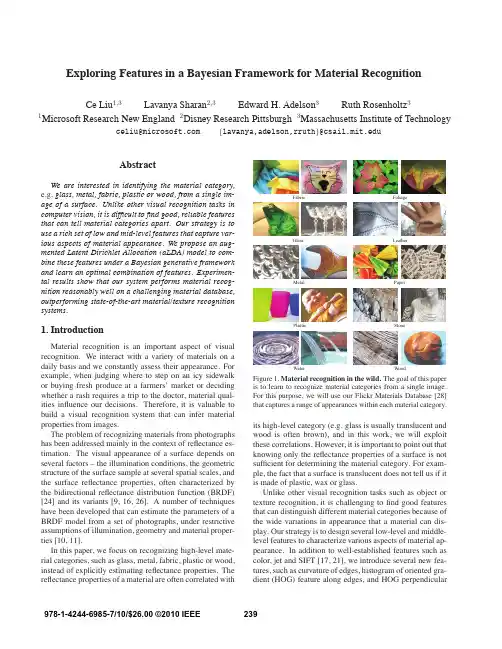
Exploring Features in a Bayesian Framework for Material Recognition Ce Liu1,3Lavanya Sharan2,3Edward H.Adelson3Ruth Rosenholtz31Microsoft Research New England2Disney Research Pittsburgh3Massachusetts Institute of Technology celiu@{lavanya,adelson,rruth}@AbstractWe are interested in identifying the material category, e.g.glass,metal,fabric,plastic or wood,from a single im-age of a surface.Unlike other visual recognition tasks in computer vision,it is difficult tofind good,reliable features that can tell material categories apart.Our strategy is to use a rich set of low and mid-level features that capture var-ious aspects of material appearance.We propose an aug-mented Latent Dirichlet Allocation(aLDA)model to com-bine these features under a Bayesian generative framework and learn an optimal combination of features.Experimen-tal results show that our system performs material recog-nition reasonably well on a challenging material database, outperforming state-of-the-art material/texture recognition systems.1.IntroductionMaterial recognition is an important aspect of visual recognition.We interact with a variety of materials on a daily basis and we constantly assess their appearance.For example,when judging where to step on an icy sidewalk or buying fresh produce at a farmers’market or deciding whether a rash requires a trip to the doctor,material qual-ities influence our decisions.Therefore,it is valuable to build a visual recognition system that can infer material properties from images.The problem of recognizing materials from photographs has been addressed mainly in the context of reflectance es-timation.The visual appearance of a surface depends on several factors–the illumination conditions,the geometric structure of the surface sample at several spatial scales,and the surface reflectance properties,often characterized by the bidirectional reflectance distribution function(BRDF) [24]and its variants[9,16,26].A number of techniques have been developed that can estimate the parameters of a BRDF model from a set of photographs,under restrictive assumptions of illumination,geometry and material proper-ties[10,11].In this paper,we focus on recognizing high-level mate-rial categories,such as glass,metal,fabric,plastic or wood, instead of explicitly estimating reflectance properties.The reflectance properties of a material are often correlatedwithFabric FoliageGlass LeatherMetal PaperPlastic StoneWater Wood Figure1.Material recognition in the wild.The goal of this paper is to learn to recognize material categories from a single image.For this purpose,we will use our Flickr Materials Database[28] that captures a range of appearances within each material category.its high-level category(e.g.glass is usually translucent and wood is often brown),and in this work,we will exploit these correlations.However,it is important to point out that knowing only the reflectance properties of a surface is not sufficient for determining the material category.For exam-ple,the fact that a surface is translucent does not tell us if it is made of plastic,wax or glass.Unlike other visual recognition tasks such as object or texture recognition,it is challenging tofind good features that can distinguish different material categories because of the wide variations in appearance that a material can dis-play.Our strategy is to design several low-level and middle-level features to characterize various aspects of material ap-pearance.In addition to well-established features such as color,jet and SIFT[17,21],we introduce several new fea-tures,such as curvature of edges,histogram of oriented gra-dient(HOG)feature along edges,and HOG perpendicular 239978-1-4244-6985-7/10/$26.00 ©2010 IEEEFigure 2.Material recognition vs.object recognition .These vehicles are made of different materials (from left to right):metal ,plastic and wood.Figure 3.Material recognition vs.texture recognition .These checkerboard patterns are made of different materials (left to right):fabric ,plastic and paper .to edges.After quantizing these features into dictionaries,we convert an image into a bag of words and use latent Dirichlet allocation (LDA)[3]to model the distribution of the words.By allowing topics to be shared amongst mate-rial categories,LDA is able to learn clusters of visual words that characterize different materials.We call our model aug-mented LDA (aLDA)as we concatenate dictionaries from various features and learn the optimal combination of the features by maximizing the recognition rate.It is crucial to choose the right image database to evaluate our system.Most existing material/texture image databases fail to capture the complexity of real world materials,be-cause they are either instance databases,such as CURET [9],or texture category databases with very few samples per class,such as KTH-TIPS2[5].The high recognition rates achieved on these databases (>95%on CURET [30])sug-gests a need for challenging,real world material databases.In this work,we use the Flickr Materials Database [28]created by us,originally for studying the visual perception of materials.This database contains 10common material categories -fabric ,foliage ,glass ,leather ,metal ,paper ,plastic ,stone ,water and wood (see Figure 1).We acquired 100color photographs from for each category,including 50close-ups and 50object-level views.All im-ages have 512×384pixel resolution and contain a single material category in the foreground.These images capture a wide range of appearances within each material category.We show that although material categorization can be a very challenging problem,especially on a database like ours,our system performs reasonably well,outperforming state-of-the-art systems such as [30].2.Related WorkRecognizing high-level material categories in images is distinct from the well-studied problem of object recogni-tion.Although object identity is sometimes predictive ofFigure 4.The projection on the first two principal components (PCs)of the texton histograms are shown for all images in the (left)61classes in the CURET database [9]and (right)10classes in the Flickr Materials Database [28].The textons were derived from 5×5pixel patches,as described in [30].The colors indicate the various texture/material categories.CURET samples are more separable than Flickr.material category,a given class of objects can be made of different materials (see Figure 2)and different classes of objects can be made of the same material (see Figure 1).Therefore,many recent advances in object recognition such as shape context [2],object detectors [7]and label transfer [19]may not be applicable for material recognition.In fact,most object recognition systems rely on material-invariant features and tend to ignore material information altogether.Material recognition is closely related to,but different from,texture recognition.Texture has been de fined in terms of dimensions like periodicity,orientedness,and random-ness [20].It can be an important component of material appearance,e.g .wood tends to have textures distinct from those of polished metal.However,as illustrated in Figure 3,surfaces made of different materials can share the same tex-ture patterns and as a consequence,mechanisms designed for texture recognition [18,30]may not be ideal for mate-rial recognition.Material recognition is also different from BRDF estima-tion.In computer graphics,there is great interest in captur-ing the appearance of real world materials.The visual ap-pearance of materials like wood or skin,has been modeled in terms of the bidirectional re flectance distribution function (BRDF)[10,22]and related representations such as BTF [9]and BSSRDF [16].Material recognition might seem trivial if the BRDF is known,but in general,it is nearly im-possible to estimate the BRDF from a single image without simplifying assumptions [10,11].A number of low-level image features have been devel-oped for identifying materials.The shape of the luminance histogram of images was found to correlate with human judgement of surface albedo [25],and was used to clas-sify images of spheres as shiny,matte,white,grey etc .[11].Similar statistics were used to estimate the albedo and gloss of stucco-like surfaces [27].Several techniques have been developed to search for speci fic materials in real world pho-tographs such as glass [15,23]or skin [14].The choice of databases is,often,the key to success in vi-240sual recognition.The CURET database[9]that consists of images of61different texture samples under205different viewing and lighting conditions,has become the standard for evaluating3-D texture classification algorithms.A vari-ety of methods based on texton representations[6,18,29], bidirectional histograms[8]and image patches[30]have been successful at classifying CURET surfaces(>95% accuracy).The KTH-TIPS2database[5]consisting of11 texture categories,4samples per category,and each pho-tographed under a variety of conditions,was introduced to increase the intra-class variation.It was shown that a SVM-based classifier achieves98.5%accuracy on this database [5].Our Flickr Materials Database[28]contains10ma-terial categories and100diverse samples in category.On inspecting the images in Figure1and the plots in Figure 4,it is apparent that the Flickr Materials Database is more challenging than the CURET database,and for this reason we chose the Flickr Materials Database to develop and eval-uate our material recognition system.3.Features for Material RecognitionIn order to build a material recognition system,it is im-portant to identify features that can distinguish material cat-egories from one another.What makes metal look like metal and wood look like wood?Is it color(neutral vs.browns), textures(smooth vs.grainy)or reflectance properties(shiny vs.matte)?Since little is known about which features are suited for material recognition,our approach is to try a vari-ety of features,some borrowed from thefields of object and texture recognition,and some new ones developed specif-ically for material recognition.From a rendering point of view,once the camera and the object arefixed,the image of the object can be determined by(i)the BRDF of the sur-face,(ii)surface structures,(iii)object shape and(iv)envi-ronment lighting.Given the diversity of appearance in the Flickr Materials Database,we will attempt to incorporate all these factors in our features.(a)Color and TextureColor is an important attribute of surfaces and can be a cue for material recognition:wooden objects tend to be brown,leaves are green,fabrics and plastics tend to be sat-urated with vivid color,whereas stones tend to be less satu-rated.We extract3×3pixel patches from an RGB image as our color feature.Texture,both of the wallpaper and3-D kind[26],can be useful for distinguishing materials.For example,wood and stone have signature textures that can easily tell them apart. We use two sets of features to measure texture.Thefirst set comprises thefilter responses of an image through a set of multi-scale,multi-orientation Gaborfilters,often called filter banks or jet[17].Jet features have been used to recog-nize3-D textures[18,30]by clustering to form textons and using the distribution of textons as a feature.The second setFigure5.Illustration of how our system generates features.(a) Curvature (b) Edge slice (HOG) (c) Edge ribbon (HOG)Figure6.We extract curvature at three scales,edge slice in6cells, and edge ribbon in6cells at edges.of features we use is SIFT[21].SIFT features have been widely used in scene and object recognition to characterize the spatial and orientational distribution of local gradients[13].(b)Micro-textureTwo surfaces sharing the same BRDF can look different if they have different surface structures,e.g.if one is smooth and the other is rough.In practice,we usually touch a sur-face to sense how rough(or smooth)it is.However,our visual system is able to perceive these properties even with-out a haptic input.For example,we can see tiny hairs on fabric,smooth surfaces in glass objects,crinkles in leather and grains in paper.In order to extract information about surface structure, we followed the idea in[1],of smoothing an image by bi-lateralfiltering[12]and then using the residual image for further analysis.The process is illustrated in Figure7.We choose three images from material categories(a)-glass, metal and fabric-and perform bilateralfiltering to obtain base image in(b)and display the residual in(d).The resid-ual of bilateralfiltering reveals variations in pixel intensity at afiner scale.For the fabric and metal example in Figure 7,the residual is due to surface structure whereas for glass, these variations are related to translucency.Although it is hard to cleanly separate the contributions of surface struc-ture from those of the BRDF,the residual contains useful information about material category.We apply the same ap-proach for characterizing the residual as we did for texture. 241(a) Original image (b) Base image (bilateral filtering) (c) Canny edges on (b) (d) Residual image: (a)-(b)(e) Edge slices(f) Edge ribbonFigure 7.Some features for material recognition .From top to bottom is glass ,metal and fabric .For an image (a)we apply bilateralfiltering [1]to obtain the base image (b).We run Canny edge detector [4]on the base image and obtain edge maps (c).Curvatures of the edges are extracted as features.Subtracting (b)from (a),we get the residual image (d)that shows micro structures of the material.We extract micro-jet and micro-SIFT features on (d)to characterize material micro-surface structure.In (e),we also show some random samples of edge slices along the normal directions of the Canny edges.These samples reveal lighting-dependent features such as specular highlights.The edge ribbon samples are shown in (f).Arrays of HOG’s [7]are extracted from (e)and (f)to form edge-slice and edge-ribbon features.We compute the jet and SIFT features of the residual image,and name them micro-jet and micro-SIFT for clarity.(c)Outline ShapeThough a material can be cast into any arbitrary shape,the outline shape of a surface and its material category are often related e.g .fabrics and glass have long,curved edges,while metals have straight lines and sharp corners.The out-line shape of a surface can be captured by an edge map.We run the Canny edge detector [4]on the base image,trim out short edges,and obtain the edge map shown in Figure 7(c).To characterize the variations in the edge maps across ma-terial categories,we measured the curvature on the edge map at three different scales as a feature (see Figure 6).(d)Re flectance-based featuresGlossiness and transparency are important cues for mate-rial recognition.Metals are mostly shiny,whereas wooden surfaces are usually dull.Glass and water are translucent,while stones are often opaque.These re flectance properties sometimes manifest as distinctive intensity changes at the edges in an image.To measure these changes,as shown in Figure 6(b),we extract histogram of oriented gradients (HOG)[7]features along the normal direction of edges.We take a slice of pixels with a certain width along the nor-mal direction,compute the gradient at each pixel,divide the slice into 6cells,and quantize the oriented gradients in to 12angular bins.This feature is called edge-slice .We also measure how the images change along the tangent directionof the edges in a similar manner,as suggested in Figure 6(c).This feature is called edge-ribbon ,which is also quan-tized by 6cells and 12angular bins for each cell.We have described a pool of features that can be po-tentially useful for material recognition:color ,SIFT ,jet ,micro-SIFT ,micro-jet ,curvature ,edge-slice and edge-ribbon .The flowchart of how our system generates these features is shown in Figure 5.Amongst these features,color,SIFT and jet are low-level features directly computed from the original image and they are often used for texture analysis.The rest of the features,micro-SIFT,micro-jet,curvature,edge-slice and edge-ribbon are mid-level features that rely on estimations of base images and edge maps (Fig-ures 7(b)&(c)).A priori,we do not know which of these features will perform well.Hence,we designed a Bayesian learning framework to select best combination of features.4.A Bayesian Computational FrameworkNow that we have a pool of features,we want to combine them to build an effective material recognition system.We quantize the features into visual words and extend the LDA [3]framework to select good features and learn per-class distributions for recognition.4.1.Feature quantization and concatenationWe use the standard k-means algorithm to cluster the in-stances of each feature to form dictionaries and map image242Figure 8.The graphical model of LDA [3].Notice that our cate-gorization shares both the topics and codewords.Different from[13],we impose a prior on βto account for insuf ficient data.features into visual words.Suppose there are m features inthe feature pool and m corresponding dictionaries {D i }m i =1.Each dictionary has V i codewords,i.e .|D i |=V i .Since fea-tures are quantized separately,the words generated by thei th feature are {w (i )1,···,w (i )N i },w (i )j ∈{1,2,···,V i }and N i is the number of words.In order to put a set of different words together,a document of m sets of words{w (1)1,···,w (1)N 1},{w (2)1,···,w (2)N 2},···,{w (m )1,···,w (m )N m }(1)can be augmented to one set{w (1)1,···,w (1)N 1,w (2)1+V 1,···,w (2)N 2+V 1,···,w (m )1+ m −1i =1V i ,···,w (m )N m + m −1i =1V i }(2)with a joint dictionary D =∪i D i ,|D |=m i =1V i .In this way,we reduced the multi-dictionary problem to a single-dictionary one.tent Dirichlet AllocationThe latent Dirichlet allocation (LDA)[3]was invented to model the hierarchical structures of words.Details of the model can be found in [3,13].In order to be self-contained,we will brie fly describe the model in the con-text of material recognition.As depicted in the graphi-cal model in Figure 8,we first randomly draw the mate-rial category c ∼Mult(c |π)where Mult(·|π)is a multino-mial distribution with parameter π.Based on c ,we select a hyper-parameter αc ,based on which we draw θ∼Dir(θ|αc )where Dir(·|αc )is a Dirichlet distribution with parameterαc .θhas the following property: ki =1θi =1where k is the number of elements in θ.From θwe can draw a se-ries of topics z n ∼Mult(z |θ),n =1,···,N .The topic z n (=1,···,k )selects a multinomial distribution βz n from which we draw a word w n ∼Mult(w n |βz n ),which cor-responds to a quantization cluster of the features.Unlike [13]where βis assumed to be a parameter,we impose a conjugate prior ηupon βto account for insuf ficient data as suggested by [3].Since it is intractable to compute the log likelihood log p (w |αc ,η),we instead maximize the lower bound L (αc ,η)estimated through the variational distributions over θ,{z d },β.Please refer to [3]for details on deriving thevariational lower-bound and parameter learning for αand η.Once we have learned αc and η,we can use Bayesian MAP criterion to choose the material categoryc ∗=arg max cL (αc ,η)+λc .(3)where λc =log πc .4.3.Prior learningA uniform distribution is often assumed for the prior p (c ),i.e .each material category will appear equally.How-ever,since we learn the LDA model for each category inde-pendently (only sharing the same β),the learning procedure may not converge in finite iterations.Therefore,the proba-bility density functions (pdfs)should be grounded for a fair comparison.We designed the following greedy algorithm to learn λby maximizing the recognition rate (or minimizing the error).Suppose {λi }i =c is fixed and we want to optimize λc to maximize the rate.Let y d be the label for document d .Let q d,i =L d (αi ,η)+λi be the “log posterior”for document d to belong to category i .Let f d =max i q d,i be the maximum posterior for document d .We de fine two sets:Ωc ={d |y d =c,f d >q d,c },Φc ={d |y d =c,f d =q d,y d }.(4)Set Ωc includes the documents that are labeled as c and mis-classi fied.Set Φc includes the documents that are not la-beled as c and correctly classi fied.Our goal is to choose λc to make |Ωc |as small as possible and |Φc |as large as pos-sible.Notice that if we increase λc ,then |Ωc |↓and |Φc |↓,therefore the optimal λc exists.We de fine the set of cor-rectly classi fied documents with λ c :sΨc ={d |d ∈Ωc ,f d <q d,c +λ c −λc }∪{d |d ∈Φc ,f d >q d,c +λ c −λc },(5)and choose the new λc that maximizes the size of Ψc :λc ←arg max λc|Ψc |.(6)We iterate this procedure for each c repeatedly until each λc does not change.4.4.Augmented LDA (aLDA)Shall we use all the features in our prede fined feature pool?Do more features imply better performance?Unfor-tunately,this is not true as we have limited training data.The more features we use,the more likely that the model over fits the training data and the performance decreases on test set.We designed a greedy algorithm in Figure 9to se-lect an optimal subset of our feature pool.The main idea is to select the best feature,one at a time,that maximizes the recognition rate on an evaluation set.The algorithm stops when adding more features will decrease the recognition rate.Note that we randomly split the training set H into L for parameter learning and E for cross evaluation.After D is learned,we use the entire training set H to relearn the parameters for D .243Input:dictionary pool{D1,···,D m},training set H •Initialize:D=∅,recognition rate r=0•Randomly split H=L∪Efor l=1to mfor D i∈D•Augment dictionary D =D∪{D i}•Concatenate words according to D using Eqn.(2)•Train LDA on L for each category(sharingβ)•Learn priorλusing Eqn.(5)and(6)•r i=recognition rate on E using Eqn.(3)endif max r i>r•j=arg max i r i,D=D∪{D j},r=r jelsebreakendend•Train LDA and learn priorλon H•r=recognition rate on HOutput:D,rFigure9.The augmented LDA(aLDA)algorithm.5.Experimental ResultsWe used the Flickr Materials Database[28]for all ex-periments described in this paper.There are ten material categories in the database:fabric,foliage,glass,leather, metal,paper,plastic,stone,water and wood.Each cate-gory contains100images,50of which are close-up views and the rest50are of views at object-scale(see Figure1). There is a binary,human-labeled mask associated with each image describing the location of the object.We only con-sider pixels inside this binary mask for material recognition and disregard all the background pixels.For each category, we randomly chose50images for training and50images for test.All the experimental results reported in this paper are based on the same split of training and test.We extract features for each image according to Figure 5.Mindful of computational costs,we sampled color,jet, SIFT,micro-jet and micro-SIFT features on a coarse grid (every5th pixel in both horizontal and vertical directions). Because there are far fewer pixels in edge maps than in the original images,we sampled every other edge pixel for cur-vature,edge-slice and edge-ribbon.Once features are ex-tracted,they are clustered separately using k-means accord-ing to the number of clusters in Table1.We specified the number of clusters for each feature,considering both di-mensionality and the number of instances per feature.After forming the dictionaries for each feature,we run the aLDA algorithm to select features incrementally.When learning the optimal feature set,we randomly split the50 training images per category(set H)to30for estimating parameters(set L)and20for evaluation(set E).After the feature set is learned,we re-learn the parameters using theFeature name Dim average#per image#of clusters Color276326.0150Jet646370.0200SIFT1286033.4250 Micro-jet646370.0200Micro-SIFT1286033.4250Curvature33759.8100Edge-slice722461.3200Edge-ribbon723068.6200 Table1.The dimension,number of clusters and average number per image for eachfeature.fabricfoliageglassleathmetalpaperplasticstonewaterwoodfabricfoliageglassleathermetalpaperplasticstonewaterwood0.10.20.30.40.50.60.70.8plastic: paperleather: fabricmetal: glass fabric: stonestonewood:glass: foliage Figure12.Left:the confusion matrix of our material recogni-tion system using color+SIFT+edge-slice feature set.Row k is the probability distribution of class k being classified to each category.Right:some misclassification bel“metal: glass”means that a metal material is misclassified as glass.50training images per category and report the training/test rate.In the LDA learning step,we vary the number of top-ics from50to250with step size50and pick the best one.The learning procedure is shown in Figure10,where for each material category we plot the training rate on the left in a darker color and test rate on the right in a lighter color.In Figure10,the recognition rate is computed on the en-tire training/test set,not just on the learning/evaluation set.First,the system tries every single feature and discovers that amongst all features,SIFT produces the highest evaluation rate.In the next iteration,the system picks up color from the remaining features,and then edge-slice.Including more features causes the performance to drop and the algorithm in Figure9stops.For thisfinal feature set“color+SIFT +edge-slice”,the training rate is49.4%and the test rate is 44.6%.The recognition rate of random guesses is10%.The boost in performance from the single best feature (SIFT,35.4%)to the best feature set(color+SIFT+edge-slice,44.6%)is due to our aLDA model that augments vi-sual words.Interestingly,augmenting more features de-creases the overall performance.When we use all the fea-tures,the test rate is38.8%,lower than using fewer features.More features creates room for overfitting,and one solution to combat overfitting is to increase the size of the database.The fact that SIFT is the best-performing single feature in-244f ab r ic f o l i a g e g l a s s l e a t h e r m e t a l p a p e r p l a s t i c s t o n e w a t e r w o o df ab r ic f o l i a g e g l a s s l e a t h e r m e t a l p a p e r p l a s t i c s t o n e w a t e r w o o df ab r ic f o l i a g e g l a s s l e a t h e r m e t a l p a p e r p l a s t i c s t o n e w a t e r w o o df ab r ic f o l i a g e g l a s s l e a t h e r m e t a l p a p e r p l a s t i c s t o n e w a t e r w o o df ab r ic f o l i a g e g l a s s l e a t h e r m e t a l p a p e r p l a s t i c s t o n e w a t e r w o o df ab r ic f o l i a g e g l a s s l e a t h e r m e t a l p a p e r p l a s t i c s t o n e w a t e r w o o df ab r ic f o l i a g e g l a s s l e a t h e r m e t a l p a p e r p l a s t i c s t o n e w a t e r w o o df ab r ic f o l i a g e g l a s s l e a t h e r m e t a l p a p e r p l a s t i c s t o n e w a t e r w o o df ab r ic f o l i a g e g l a s s l e a t h e r m e t a l p a p e r p l a s t i c s t o n e w a t e r w o o df ab r ic f o l i a g e g l a s s l e a t h e r m e t a l p a p e r p l a s t i c s t o n e w a t e r w o o df ab r ic f o l i a g e g l a s s l e a t h e r m e t a l p a p e r p l a s t i c s t o n e w a t e r w o o df ab r ic f o l i a g e g l a s s l e a t h e r m e t a l p a p e r p l a s t i c s t o n e w a t e r w o od Figure 10.The per-class recognition rate (both training and test)with different sets of features for the Flickr database [28].In each plot,the left,darker bar means training,the right,lighter bar means test.For the two numbers right after the feature set label are the recognition rate on the entire training set and the rate on the entire test set.For example,“color:37.6%,32.0%”means that the training rate is 37.6%and the test rate is 32.0%.Our aLDA algorithm finds “color +SIFT +edge-slice”to be theoptimal feature set on the Flickr Materials Database.f ab r ic f o l i a g e g l a s s l e a t h e r m e t a l p a p e r p l a s t i c s t o n ew a t e r w o o d f ab r ic f o l i a g e g l a s s l e a t h e r m e t a l p a p e r p l a s t i c s t o n e wa t e r w o o d f ab r ic f o l i a g e g l a s s l e a t h e r m e t a l p a p e r p l a s t i c s t o n e wa t e r w o o d f ab r ic f o l i a g e g l a s s l e a t h e r m e t a l p a p e r p l a s t i c s t o n e wa t e r w o o d f ab r ic f o l i a g e g l a s s l e a t h e r m e t a l p a p e r p l a s t i c s t o n e wa t e r w o o d f ab r ic f o l i a g e g l a s s l e a t h e r m e t a l p a p e r p l a s t i c s t o n e wa t e r w o o d f ab r ic f o l i a g e g l a s s l e a t h e r m e t a l p a p e r p l a s t i c s t o n ew a t e r w o o d f ab r ic f o l i a g e g l a s s l e a t h e r m e t a l p a p e r p l a s t i c s t o n e wa t e r w o o d f ab r ic f o l i a g e g l a s s l e a t h e r m e t a l p a p e r p l a s t i c s t o n e wa t e r w o o d f ab r ic f o l i a g e g l a s s l e a t h e r m e t a l p a p e r p l a s t i c s t o n ew a t e r w o o d f ab r ic f o l i a g e g l a s s l e a t h e r m e t a l p a p e r p l a s t i c s t o n ew a t e r w o o d f ab r ic f o l i a g e g l a s s l e a t h e r m e t a l p a p e r p l a s t i c s t o n e w a t e r w o od Figure 11.For comparison,we run Varma-Zisserman’s system [30](nearest neighbor classi fiers using histograms of visual words)on our feature sets.Because of the nearest neighbor classi fier,the training rate is always 100%,so we simply put it as N/A.dicates the importance of texture in material recognition.In addition,SIFT also encapsulates some of the informa-tion captured by micro-SIFT.Edge-slice,which measures re flectance features,is also useful.For comparison,we implemented and tested Varma-Zisserman’s (VZ)algorithm [30]on the Flickr Materials Database.The VZ algorithm clusters 5×5pixel gray-scale patches as codewords,obtains a histogram of the codewords for each image,and performs recognition using a nearest neighbor classi fier.As a sanity check,we ran our im-plementation of VZ on the CURET database and obtained 96.1%test rate (their numbers are 95∼98%,[30]).Next,we ran the exact VZ system tested on CURET on the Flickr Materials Database.The VZ test rate is 23.8%.This sup-ports the conclusions from Figure 4that the Flickr Materials Database is much harder than the CURET texture database.As the VZ system uses features tailored for the CURET database (5×5pixel patches),we ran VZ’s algorithm using our features on Flickr Materials Database.The results of running VZ’s system on exactly the same feature sets as inFigure 10are listed in Figure 11.Since VZ uses a nearest neighbor classi fier,it is meaningless to report the training rate as it is always 100%,so we only report the test rate.It is obvious why many of our features outperform fixed size gray-scale patch features on Flickr Materials Datatbase.In fact,the VZ system running on SIFT features has test rate of 31.8%,close to our system using SIFT alone (35.2%).However,combining features under the VZ’s framework only slightly increases the performance to a maximum of 37.4%.Clearly,the aLDA model contributes to the boost in performance from 37.4%to 44.6%.The confusion matrix of our system (color +SIFT +edge-slice,test rate 44.6%)in Figure 12tells us how often each category is misclassi fied as another.For example,fab-ric is often misclassi fied as stone ,leather misclassi fied as fabric ,plastic misclassi fied as paper .The category metal is more likely to be classi fied as glass than itself.Some misclassi fication examples are shown in Figure 12.These results are not surprising because there are certain common-alities between leather and fabric ,plastic and paper ,as well245。


遥感图像的分类与特征提取方法遥感图像处理是一项重要的技术,可以帮助我们更好地理解和利用地球表面的信息。
其中,遥感图像的分类与特征提取方法是关键的研究方向。
本文将探讨这一主题,介绍常见的分类和特征提取方法,并讨论各种方法的优劣以及适用场景。
一、常见的遥感图像分类方法遥感图像的分类是将图像像素按照其代表的地物类别进行划分和识别。
常见的分类方法包括像素级分类、对象级分类和混合分类。
1. 像素级分类:像素级分类是将图像中的每个像素点都进行分类。
该方法适用于较小的地物或者需要保留细节信息的需求场景。
常见的像素级分类方法包括支持向量机(SVM)、最大似然分类和随机森林分类等。
2. 对象级分类:对象级分类是将图像中的连续区域作为分类单元,对整个区域进行分类。
这种方法可以更好地利用图像中的上下文信息,提高分类精度。
常见的对象级分类方法有基于区域的卷积神经网络(RCNN)、基于区域的卷积神经网络(R-CNN)和卷积神经网络(CNN)等。
3. 混合分类:混合分类方法是将像素级分类和对象级分类相结合,综合利用两者的优点。
例如,可以先进行像素级分类得到初步分类结果,再通过对象级分类对初步结果进行修正和细化。
这种方法可以在保留细节信息的同时,提高分类的准确性和鲁棒性。
二、常见的遥感图像特征提取方法特征提取是遥感图像分类的关键环节,通过提取图像中的特征信息,可以更好地描述和区分不同地物类别。
常见的特征提取方法包括光谱特征提取、纹理特征提取和形状特征提取等。
1. 光谱特征提取:光谱特征是指通过对图像中每个像素点的光谱反射率进行分析和处理,提取出的表示不同地物的特征。
常见的光谱特征提取方法有主成分分析(PCA)、线性判别分析(LDA)和维度约简等。
2. 纹理特征提取:纹理特征是指图像中不同地物的纹理差异。
通过对图像的纹理进行分析和提取,可以更好地区分不同地物。
常见的纹理特征提取方法有灰度共生矩阵(GLCM)、局部二值模式(LBP)和方向梯度直方图(HOG)等。
第六章遥感图像判读及分类遥感图像的核心问题是根据辐射能在各种图像上的表现特征,判读出地面特征。
所谓判读就是对图像中内容进行分析,判读、解释,弄清楚图像中的线条、轮廓、色彩、花纹等内容对应着地表上的什么景物及这些景物处于什么状态。
遥感判读是遥感技术的重要内容之一。
判读最基本方法有两种,即目视判读和电子计算机自动识别和分类。
§6—1 遥感图像的目视判读一、景物特征与判读标志景物特征主要有光谱特征,空间特征和时间特征,此外在微波区还有偏振性。
景物的这些特征在影像上以灰度变化的形式表现出来。
不同的地物,这些特征不同,在影像上的表现形式也不同,因此,可根据影像上的变化和差别来区分不同类别,再根据其经验,知识和必要的资料,判读地物的性质或一些自然现象。
各种地物在影像上的各种特有的表现形式称为判读标志(image interpretation)。
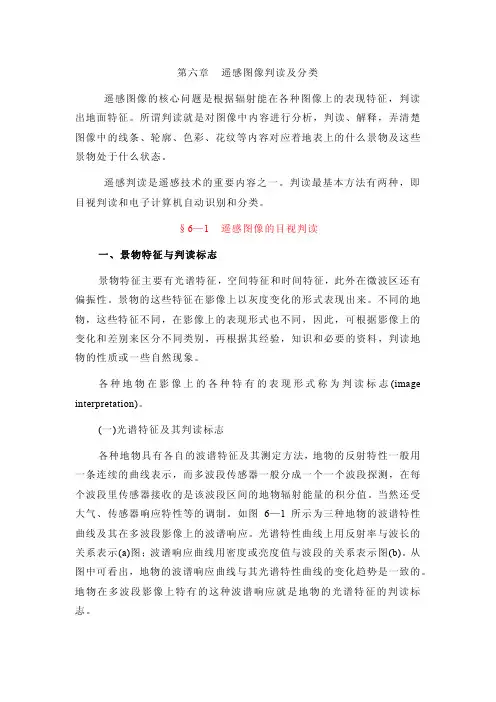
(一)光谱特征及其判读标志各种地物具有各自的波谱特征及其测定方法,地物的反射特性一般用一条连续的曲线表示,而多波段传感器一般分成一个一个波段探测,在每个波段里传感器接收的是该波段区间的地物辐射能量的积分值。
当然还受大气、传感器响应特性等的调制。
如图6—1所示为三种地物的波谱特性曲线及其在多波段影像上的波谱响应。
光谱特性曲线上用反射率与波长的关系表示(a)图;波谱响应曲线用密度或亮度值与波段的关系表示图(b)。
从图中可看出,地物的波谱响应曲线与其光谱特性曲线的变化趋势是一致的。
地物在多波段影像上特有的这种波谱响应就是地物的光谱特征的判读标志。
(二)空间特征及其判读标志景物的各种几何形态为其空间特征,它通常包括目视判读中应用的一些判读标志。
1.直接判读标志(1)形状影像的形状是物体的一般形式或轮廓在图像上的反映。
各种物体具有一定的形状和特有的辐射特性。
同种物体在图像上有相同的灰度特性,这些同灰度的像素在图像上的分布就构成与物体相似的形状。
随图像比例尺的变化,“形状”的含义也不同。
实验四遥感图像分类一、背景知识图像分类就是基于图像像元的数据文件值,将像元归并成有限几种类型、等级或数据集的过程。
常规计算机图像分类主要有两种方法:非监督分类与监督分类,本实验将依次介绍这两种分类方法。
非监督分类运用ISODATA(Iterative Self-Organizing Data Analysis Technique)算法,完全按照像元的光谱特性进行统计分类,常常用于对分类区没有什么了解的情况。
使用该方法时,原始图像的所有波段都参于分类运算,分类结果往往是各类像元数大体等比例。
由于人为干预较少,非监督分类过程的自动化程度较高。
非监督分类一般要经过以下几个步骤:初始分类、专题判别、分类合并、色彩确定、分类后处理、色彩重定义、栅格矢量转换、统计分析。
监督分类比非监督分类更多地要用户来控制,常用于对研究区域比较了解的情况。
在监督分类过程中,首先选择可以识别或者借助其它信息可以断定其类型的像元建立模板,然后基于该模板使计算机系统自动识别具有相同特性的像元。
对分类结果进行评价后再对模板进行修改,多次反复后建立一个比较准确的模板,并在此基础上最终进行分类。
监督分类一般要经过以下几个步骤:建立模板(训练样本)分类特征统计、栅格矢量转换、评价模板、确定初步分类图、检验分类结果、分类后处理。
由于基本的非监督分类属于IMAGINE Essentials级产品功能,但在IMAGINE Professional级产品中有一定的功能扩展,非监督分类命令分别出现在Data Preparation菜单和Classification菜单中,而监督分类命令仅出现在Classification菜单中。
二、实验目的理解并掌握图像分类的原理,学会图像分类的常用方法:人工分类(目视解译)、计算机分类(监督分类、非监督分类)。
能够针对不同情况,区别使用监督分类、非监督分类。
理解计算机分类的常用算法实现过程。
熟练掌握遥感图像分类精度评价方法、评价指标、评价原理,并能对分类结果进行后期处理。