人口统计学4-20121109-学生
- 格式:ppt
- 大小:2.56 MB
- 文档页数:70


人口统计学知识:人口普查和民意调查中的数据收集与处理技术人口统计学知识:人口普查和民意调查中的数据收集与处理技术在现代社会,人口统计学越来越重要。
人口普查和民意调查是人口统计学的两个重要研究领域。
人口普查是一项全国性的、统计全国人口数量、结构、分布和通用生活状况的调查,而民意调查则是在特定的群体中进行的调查,以了解他们的看法和意见。
在人口普查和民意调查中,数据是收集和处理的关键。
本文将重点介绍数据收集和处理技术,以帮助人们更好地理解这些重要的人口统计学领域。
一、人口普查中的数据收集人口普查通常通过以下三种方式来收集数据:纸质问卷、个人面谈和电话访问。
纸质问卷法是人口普查中最常用的方法之一。
普查机构会将包含问卷的信封寄到每个家庭,居民填写后邮寄回普查机构。
由于纸质问卷法的优缺点各有,因此它也有一些局限性。
优点是:比较方便和低成本;问卷也可以像标准程序一样印刷和复制。
缺点是:人们填写问卷的精度不高,也有可能造成数据缺失或错误,人口普查员需要耗费体力和时间进行清点和核实。
个人面谈法质量较高,但成本也高。
在这种方式下,普查员会亲身拜访每个家庭,填写每个家庭的人口数、性别、年龄、教育水平等信息。
尽管这是最准确的方法之一,但它却是最昂贵和最费时的课题。
电话访问法是一种相对较新的方式。
这是通过电话与普查对象进行沟通,咨询一些人口统计数据。
这种方式虽然成本较低,但也存在缺点。
一些家庭可能没有电话,或者可能存在虚假回答,这将导致数据不准确。
二、人口普查的数据处理技术人口普查数据分析和处理也是必不可少的步骤。
这些数据可能包括人口数量、性别、年龄、婚姻状态、民族、职业、家庭收入和社会福利。
这些数据的分析和处理可以帮助政府和相关机构更好地了解人口的趋势和需要,从而做出科学和有效的决策。
1.数据输入:首先,需要将普查数据输入计算机,并对其进行数字化处理。
数字化处理是将普查信息转换为数码形式,以便更方便地存储、分析和处理这些数据。

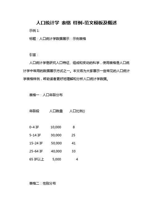
人口统计学表格样例-范文模板及概述示例1:标题:人口统计学数据展示:示例表格引言:人口统计学是研究人口特征、组成和变动的科学,使用表格是人口统计学中常用的数据展示方式之一。
本文将为大家展示一些常见的人口统计学表格样例,帮助读者更好地理解和分析人口统计学数据。
表格一:人口年龄分布年龄段人口数量人口比例()0-4岁10,000 85-14岁30,000 2515-24岁50,000 4125-64岁40,000 3365岁以上5,000 4表格二:性别分布性别人口数量人口比例()男性60,000 50女性60,000 50表格三:人口教育水平教育水平人口数量人口比例()小学10,000 8初中20,000 17高中25,000 21本科45,000 37研究生20,000 17表格四:人口就业状况就业状况人口数量人口比例() 在职80,000 67失业10,000 8退休20,000 17自由职业10,000 8结论:以上是人口统计学中常见的表格样例,我们可以通过这些表格了解到人口的年龄分布、性别分布、教育水平和就业状况等重要信息。
通过对这些数据的分析,我们可以更好地理解和应对人口变动和特征,为决策制定和资源分配提供有力支持。
示例2:人口统计学是一门研究人口数量、结构、分布和变动等问题的学科,它通过收集、整理和分析大量的人口数据来揭示人口发展的规律和趋势。
在这篇文章中,我们将展示一个人口统计学表格样例,以便读者更好地理解和应用这些数据。
以下是一个简单的人口统计学表格样例:年份总人口城市人口农村人口出生率死亡率城市化率- -2000 1000 400 600 10‰5‰402005 1200 500 700 8‰4‰41.72010 1500 600 900 7‰3‰402015 1800 700 1100 6‰ 2.5‰38.92020 2000 800 1200 5‰2‰40在这个表格中,我们可以看到不同年份的总人口、城市人口、农村人口、出生率、死亡率和城市化率的数据。
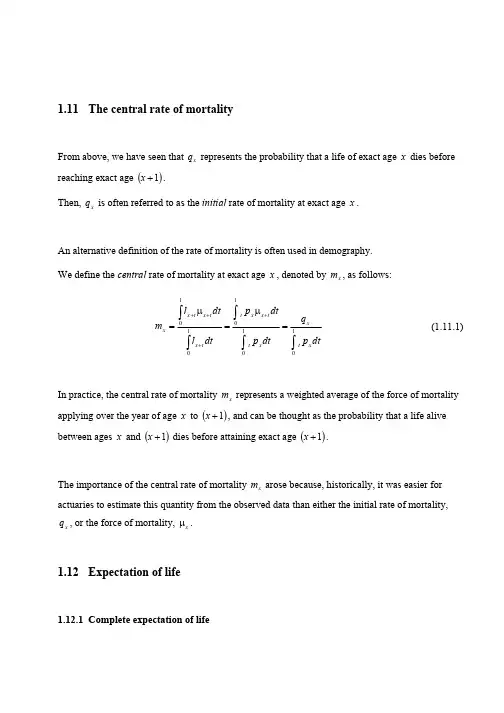
1.11 The central rate of mortalityFrom above, we have seen that q represents the probability that a life of exact age dies before reaching exact age .x x ()1+x Then, q is often referred to as the initial rate of mortality at exact age . x xAn alternative definition of the rate of mortality is often used in demography. We define the central rate of mortality at exact age , denoted by , as follows:x x m ∫∫∫∫∫=µ=µ=++++11111dtp q dtp dtp dtldtlm x txx tt x x t tx t x t x x(1.11.1)In practice, the central rate of mortality represents a weighted average of the force of mortality applying over the year of age to (, and can be thought as the probability that a life alive between ages and ( dies before attaining exact age (). x m )1x +x x )1+x 1+xThe importance of the central rate of mortality arose because, historically, it was easier for actuaries to estimate this quantity from the observed data than either the initial rate of mortality, , or the force of mortality, . x m x q x µ1.12 Expectation of life1.12.1 Complete expectation of lifeFrom Section 1.2, the random variable T represents the complete future lifetime for a life of exact age .x x Then, the expected value of the random variable T , denoted by e , is the complete expectation of life for a life of age .x ox x From (1.5.4), the probability density function of the random variable T is given by:x ()t x x t x p t f +µ= for 0≥tNote that is the expected future lifetime after age , so that, for a life of exact age , theexpected age at death is .ox e x x+ox e x Now, by definition, we have:()()∫∫∞+∞µ×=×==0odt p t dt t f t T E e t x x t x x x(1.12.1)Then, from (1.5.5), we havet x x t x t p p t+µ=−∂∂, and using integration by parts, we obtain: ()[]()∫∫∫∫∞∞∞==∞∞+=−−−×= ∂∂−×=µ×=0000odtp dt p p t dt p t t dtp t e x tx t t t x t x t tx xtx(1.12.2)Example 1.12.12In a particular survival model, we have:xx 01.0101.0−=µ for 0<≤x100Find the complete expectation of life at exact age 20. SolutionFirstly, we must find t , the survival function for a life of exact age 20. 20p From (1.7.1), we have:()[]()()8012001.0101.012001.012001.0101.01ln exp 01.0101.0exp exp 20202020202020ttt s ds s ds p ts s t t s t−=×−−=×−+×−=−−−=−−=µ−=+==++∫∫As the limiting age in the survival model is 100, the complete future lifetime for a life of exact age 20 must be less than 80 years. Then, from (1.8.2), we have:4040801800280020-100020o20=−=−====∫∫t t tt t dt t dtp e 3Thus, the complete expectation of life for a life of exact age 20 is 40 years.The complete expectation of life, typically for a new-born life, is often used to compare the general level of health in different populations.For example, the life expectancy for a new-born male life in different countries is:Country Life expectancy Japan 77.5 United Kingdom 75.0 Germany 74.3 United States74.2Mexico 68.5 Russia 62.0 South Africa50.4Zimbabwe 39.2Source: US Bureau of the Census, International data base, June 2000Also, using integration by parts, it can also be seen that:()∫∫∞∞+××=µ×=0222dt p t dt p tTE x t t x x t xThus, the variance of the complete future lifetime for a life of exact age is given by:x ()()()[]200222var−××=−=∫∫∞∞dt p dt p t T E T E T x t x t x x x(1.12.3)41.12.2 Curtate expectation of lifeThe random variable is used to represent the curtate future lifetime for a life of exact age (i.e. the number of complete years lived after age ).x K x x Then, the random variable is the integer part of the complete future lifetime, T . x K x Clearly, is a discrete random variable taking values in the state space .x K …,2,1,0=J We can use the distribution function of T , denoted by , to derive the probability distribution function of as follows:x ()t F x x K ()(()()()(()))xk x kx x kx x kx k x kx k x k x x x x l d q p p p p p p p k F k F k T k k K +++++=×=−×=−=−−−=−+=+<≤==11111111Pr Pr(1.12.4)This result is intuitive.If the random variable takes the value , then a life of exact age must live for complete years after age . Therefore, the life must die in the year of age to ().x K k x ()k k x x +1++k x From above, we have seen that, for a life of exact age , the probability of death in the year of ageto is x ()k x +()1++k x ()k K l d q x xkx xk ===+Pr .5Now, the expected value of the random variable , denoted by , is known as the curtate expectation of life for a life of age . x K x e x Thus, we have:()()()()()∑∑∑∞=++++++++++++∞=+∞==+++=+−×+−×+−=+×+×+=×==×==1321433221321003232Pr k xkxx x x xx x x x x x xx x x k xkx k xx xp l l l l l l l l l l l l d d d l d k k Kk K E e ………(1.12.5)If required, we can also calculate the variance of the curtate future lifetime as follows:()()()[]()∑∞=+−×=−=02222var k x xk x xxx e l d kK E KE K (1.12.6)1.12.3 Relationship between e and ox x eAssuming that the function t is linear between integer ages, we have:x p 6()()212121211021100o+=+×=++×++×≈=∑∫∞=∞x k xk x x x x x x txe p p p p p p dtp e … (1.12.7)Thus, the complete expectation of life at age is approximately equal to the curtate expectation of life plus one-half of a year.x This is equivalent to the assumption that lives dying in the year of age to () do so,on average, half-way through the year at age ()k x +1++k x ().21++k x This assumption is known as the uniform distribution of death assumption.It should be noted that, whilst the curtate future lifetime is equal to the integer part of the complete future lifetime T , the curtate expectation of life is not equal to the integer part of the complete expectation of life . x K e x x ox e1.13 Interpolation for the life tableAs discussed previously, it is common for the standard life table functions such as l , or µ to be tabulated at integer ages only.x x q x However, the actuary may be required to calculate probabilities involving non-integer ages or durations.Then, given a life table { specified only at integer ages, how can we approximate the values of (where is an integer and )? }ω+αα=,,1,:…x l x t x l +x 10<<t We consider three possible approaches.71.13.1 Uniform distribution of deaths (UDD)In this case, we assume that any deaths over the year of age to occur uniformly over the year.x (1+x ))This is equivalent to the assumption that the function l is linear over the interval (). t x +1,+x x Thus, for 0, we have l 1<<t ()()x x x x x x x t x d t l l l t l l t l t ×−=−×−=×+×−=+++111.Hence, under the UDD assumption, dividing both sides by gives:x l x x t x t x x tq t p q q t p ×=−=⇒×−=11Then, under the assumption that the function l is linear over the interval (, we have:t x +1,+x x x ts x x s x tq t ds p q ×=µ=∫+0(1.13.1)Thus, as the function q is tabulated, we can estimate the probability t for any non-integer durations t .x x q Note that, differentiating both sides of this expression with respect to t , we obtain:()t f p ds p dt d q x t x x t ts x x s x =µ=µ=++∫0for 0<<t 1Thus, under the assumption that the function is linear over the interval , the distribution function of the complete future lifetime, T , is constant for 0. t x l +()1,+x x 1<t x <Hence, deaths are uniformly distributed over the year of age to . x ()1+x8We can extend this approach when both the age and the duration are non-integer values, so as to enable us to estimate the probability t where is an integer and 0). s x s q +−x 1<<<t s In this case, we can write xs xts x s t s x s t x s x p p p p p p =⇒×=+−+−t . Thus, we can express t as s x s q +−x s x t xs x ts x s t s x s q qp p p q −−−=−=−=+−+−11111.tAnd, using the UDD assumption, we have:()xxx x sx st q s q s t q s q t q ×−×−=×−×−−=+−1111 f 1or<<<t s (1.13.2)Also, using the UDD assumption, we can express the central rate of mortality at age , , in twodifferent ways:x x m (i)If the function t is linear for 0, then we have x p 1≤≤t x x t p dt p 11=∫ (i.e. the value ofthe function t at the mid-point of the interval). Thus, we have:x p x xx x xx x txx q q q q p q dtp q m ×−=−===∫2111111 (1.13.3)(ii)If the function is constant for 0, then we can put ()t x x t x p t f +µ=1≤≤t 21=t giving ()2121+µ=x x x p t f for all t . Thus, we have:[1,0∈]21121211212111110++++µ=×µ=µ=µ=∫∫∫∫x xx x xx x x tt x x t x p dtp p dtp dtp dtp m(1.13.4)1.13.2 Constant force of mortality9In this case, we assume that the function µ is constant over the year of age to (). t x +x 1+x i.e. for integer and , we have µ x 10<<t constant =µ=+t xNote that, in general, the value of µ, the constant force of mortality assumed over the year of age to , will not be equal to either of the tabulated values µ or µ. x (1+x )x 1+xUnder the assumption of a constant force of mortality between integer ages, we find the value of the constant µ using:()x t x x p e dt p ln exp 10−=µ⇒=µ−=µ−+∫ (1.13.5)Then, for 0, we have:1<<t µ−+−=µ−−=µ−−=−=∫∫t t t s x xt x te ds ds p q 1exp 1exp 1100 (1.13.6)Similarly, when we have a non-integer age and duration, we estimate the probability t , for , as follows:s x s q +−10<<<t s ()µ−−++−+−−=µ−−= µ−−=−=∫∫s t t s t s r x sx s t s x st e dr dr p q 1exp 1exp 11 (1.13.7)10Example 1.9.1Given , calculate 75.090=p 90121q and 121190121qassuming:(a) a uniform distribution of deaths between integer ages, and (b) a constant force of mortality between integer ages. Solution (a)Uniform distribution of deathsFrom (1.13.1), we have:()()020833.025.011211121121909090121=−×=−×=×=p q qAlso, from (1.13.2) with 1211=s and t , we have: 1=027027.025.01211125.012112111121119090121190121=×−×=×−× −=q q q(b)Constant force of mortalityFirst, we must find the value of , the constant force of mortality over the year of age (). µ91,90Then, from (1.13.5), we have µ. ()()287682.075.0ln ln 90=−=−=p From (1.13.6), we have:023688.0112190121=−=µ×−eqAlso, from (1.13.7) with 1211=s and t , we have: 1=11023688.01112112111121190121=−=−=µ−µ×−−e eqNote that, under the constant force of mortality assumption, the central rate of mortality at age , , is given by:x x m µ=×µ=µ=∫∫∫∫+11011dtp dtp dtp dtp m x tx t x tt x x t x(1.13.8)1.13.3 The Balducci assumptionThe Italian actuary Balducci proposed an alternative approach for estimating probabilities at non-integer ages and durations.The approach is based on the traditional actuarial method of constructing a life table, which will be considered in more detail later.The assumption is that the function l is in form hyperbolic between integer ages.t x +Note that, as mentioned previously, the UDD assumption implies that the function l is linear between integer ages, whereas the constant force of mortality assumption implies that the function is exponential between integer ages. t x +t x l +Then, for any integer and 0, using hyperbolic interpolation, we have x 1<<t 111+++−=x x tx l tl t l . Thus, for 0, we can write:1<<t 12()()()xx x x t x x x x xx tx l l l t l l l l l l t l t l 1111111++++++−×−−=⇒××+×−=Hence, the Balducci assumption is usually expressed as:()()()x t x t t x t x xxt x tq t p q q t l d t p ×−=−=⇒×−−=×−−=+−+−+−111111111 (1.13.9)Now, using the Balducci assumption, we have:()x xtx t x x t t x t xx t t x t x t x q t q p p q p p p p p p ×−−−−=−=⇒=⇒×=+−+−+−11111111Hence, for integer age and 0, the Balducci assumption gives:x 1<<t ()()xxx x x t q t q t q t q q ×−−×=×−−−−=111111 (1.13.10)By definition, the assumption of a constant force of mortality assumes that the function is constant over the year of age to ().t x +µx 1+x Now, combining (1.2.5) and (1.3.4), we have ()t x tx t x l dtdl +++×−=1µ.For the UDD assumption, we have ()()(11++++−−=⇒−×−=x x t x x x x t x l l l dt dl l t l ))l . Thus, using the UDD assumption, we can express the force of mortality at age as:(t x +()xxx x x x x t x q t q l l t l l l ×−=−×−−=µ+++111(1.13.11)13Thus, under the UDD assumption, the force of mortality is an increasing function over the year of age to .x ()1+x This result can be explained by general reasoning.Consider a group of lives who die at a uniform rate over a given year.Then, to maintain a constant number of deaths over the year, the force of mortality must increase to offset the fact that the number of survivors is decreasing over time.Also, this result is intuitive and consistent with the expected pattern for the force of mortality for human populations (i.e. we expect the force of mortality to be an increasing function of age).Similarly, for the Balducci assumption, it can shown that the force of mortality at age () is given by:t x +()xxt x q t q ×−−=µ+11(1.13.12)Thus, under the Balducci assumption, the force of mortality is a decreasing function over the year of age to .x ()1+x This result is counter-intuitive and inconsistent with the expected pattern for the force of mortality for human populations.However, as mentioned previously, the assumption is useful in the traditional actuarial method of constructing a life table (and will be considered further later).1.14 Simple analytical laws of mortalityIt may be possible to postulate an analytical form for one of the standard life table functions such as l , or µ.x x q x 14Such an approach simplifies the construction of a suitable life table from crude mortality data (as the number of parameters required to be estimated is substantially reduced), but the mathematical formulae used must be representative of the actual underlying mortality experience (and is now considered unlikely that a simple analytical expression can be proposed that will adequately represent human mortality over a large range of ages).However, before the recent advancements in computing speed and storage capacity, this approach was reasonably common and we now consider some of better-known laws of mortality proposed.1.14.1 De Moivre’s LawDe Moivre’s Law was proposed in 1729 and states that, for all ages such that 0, wehave:x ω<≤x xx −ω=µ1(1.14.1)Thus, as expected, the force of mortality is an increasing function of age.Then, we can derive the survival function as follows:()[]()()xt x s ds s ds p tx s x s t x x t x x s xt−ω+−ω=−ω= −ω−=µ−=+==++∫∫ln exp 1exp exp (1.14.2)1.14.2 Gompertz’ Law15Gompertz’ Law was proposed in 1829 and was based on the observation that, over a large range of ages, the function µ is log-linear. x Thus, for all ages , we have:0≥x x x Bc =µ(1.14.3)Then, assuming that the underlying force of mortality follows Gompertz’ Law, the parameter values and can be determined given the value of the force of mortality at any two ages. B c To ensure that the force of mortality is a non-negative increasing function of age, we require that the parameter values and are such that and . B c 0>B 1>cWe can derive the survival function as follows:()()()[]()()−−=−=−=−=µ−===++∫∫∫1ln exp ln exp exp exp exp 0ln 0ln 00t x t s s c s x t c s x t sx t s x xtc c c B e c c B ds e Bc ds Bc ds pNow, if we define the parameter such that g ()−=c B g ln exp , then we can express the survivalfunction as:()()[]()11ln exp −=−=tx c c t x x tg c c g p(1.14.4)16In practice, Gompertz’ Law is often found to be a reasonable approximation for the force of mortality at older ages.1.14.3 Makeham’s LawMakeham’s Law was proposed in 1860, and incorporated the addition of a constant term in the expression for the force of mortality.The rationale behind this is that an age-independent allowance is required for the incidence of accidental deaths.Thus, for all ages , we have:0≥x x x Bc A +=µ(1.14.5)Then, assuming that the underlying force of mortality follows Makeham’s Law, the parameter values , and can be determined given the value of the force of mortality at any three ages. A B c To ensure that the force of mortality is a non-negative increasing function of age, we require that the parameter values , and are such that , and . A B c B A −≥0>B 1>cWe can derive the survival function using the same approach adopted above for Gompertz’ Law to obtain:()1−=tx c c t x tg s p(1.14.6)where and (A s −=exp )()−=c B g ln exp .Example 1.14.1A survival model is assumed to follow Makeham’s Law for the force of mortality at age , µ.x x 17Then, given that , and , find the values of the parameters , and .70.0705=p 40.0805=p 15.0905=p A B c Hence, or otherwise, find the probability that a life of exact age 50 will die between exact ages 55 and 65. SolutionFrom (1.14.6), we have:()()()()()()315.0240.0170.0159051580515705590580570−−−==−−−==−−−==−−−c c c c c c g s p g s p g s pThus, we have:()()()()()()()()()()540.015.023470.040.01211115108051070−−−=⇒−−−=⇒−−−−c cc c c c g gThen, taking logarithms of (4) and (5) gives:()()()()()()()()740.015.0ln ln 11670.040.0ln ln 115108051070−−−=×−−−−−=×−−g c c c g c c cAnd, dividing ( by ( gives:)7)6057719.170.040.0ln 40.015.0ln 10=⇒=c c18Then, from , we have ()4()()()955824.0045181.01170.040.0ln 51070=⇒−=−− =g c c c g ln . Now, from (1.14.6), we have ()002535.0ln exp =⇒−=B c B g .And, taking the logarithm of (, gives:)1()()()()()077364.0ln ln 1ln 570.0ln 570=⇒×−+×=s g c c sFrom (1.14.6), we have . ()077364.0exp −=⇒−=A A sThus, the force of mortality at age is given by .x ()xx 057719.1002535.0077364.0×+−=µ1.15 The select mortality tableBefore being accepted for life assurance cover, potential policyholders are often required to undergo a medical examination to satisfy the insurer that they are in a ‘reasonable’ level of health. Lives who fail to satisfy the requirements laid down by the insurance company will often be refused cover (or required to pay a higher premium for the same level of cover).As a result of this filtering, lives who have recently been accepted for cover can be expected to be in better health (and, thus, experience lighter mortality) than the general population at the same age.This effect is known as selection (i.e. the process of choosing lives for membership of a defined group, rather than random sampling).19However, as the duration since selection increases, the extent of the lighter mortality experienced by the select group of lives can be expected to reduce (as previously healthy individuals are exposed to the same medical conditions as the general population).In practice, select lives are often assumed to experience lighter mortality for a period of, say,s years (known as the select period). However, once the duration since selection exceeds the select period, the lives are assumed to experience the ultimate mortality rates appropriate for the general population at the same age.Thus, we now consider the construction and application of a select life table, where mortality varies by age and duration since selection.The A1967-70 mortality table uses a select period of two years, so that select lives are assumed to experience lighter mortality for the first two years after selection (before reverting to the mortality experience of the general population, as represented by the ultimate portion of the table). However, the a(55) table uses a select period of one yearAnd, the ELT No. 15 – Males table is an ultimate life table only (i.e. there is no select period). This is commonly referred to as an aggregate mortality table.Examples of selection include:(a) temporary initial selection- that exercised by a life assurance company in deciding whether or not to accept a person for life assurance cover- selection takes place by producing satisfactory medical evidence- known as underwriting(b) self selection- that exercised by lives when choosing to purchase an annuity (i.e. exchanging a capital sum for the receipt of an income for life)20These are examples of positive selection , where the select lives are likely to experience lower mortality rates than the general (or ultimate ) population of the same age for a specified duration since selection only.However, a life retiring early on grounds of ill-health is likely to experience higher mortality than the ultimate population of the same age. This is an example of negative selection .1.15.1 Select, ultimate and aggregate mortality ratesMost select life tables are constructed to explore the effect of temporary initial selection (i.e. where selected lives experience lighter mortality than the general population studied for a specified duration since selection).Suppose that the select period is years.s Consider a life who is currently of exact age (, and who was selected at age . )))r x +x Thus, the duration since selection is years.r Now, if r , then we expect the life to experience lower mortality than the ultimate population at the same age and we define the select mortality rate at age as follows:s <(r x +[]()([]1 age before dies , age at group select joined who , aged now life Pr +++=+r x x r x q r xNote that is used to denote the age at selection and r is the duration since selection, so that the current age of the life is .[]x ()r x +Thus, as the life is expected to experience lower mortality than an ultimate life of the same age, we have:[]r x r x q q ++< for r <s (1.15.1)And, as before, we have [][]r x r x q p ++−=1.21Similarly, consider another life who is also currently of exact age , but who was selected at age ().(r x +))))])))1+x Thus, in this case, the duration since selection is years.(1−r We define the select mortality rate at age for this life as follows:(r x +[]()()()([]1 age before dies ,1 age at group select joined who , aged now life Pr 11++++=−++r x x r x q r xNote that, in this case, [ is used to denote the age at selection and ( is the duration since selection, so that the current age of the life is also (). 1+x 1−r r x +However, as this life has been selected more recently, we would expect this life to experience lighter mortality over the year of age to ( than the life selected at age . ()r x +1++r x x Thus, we have:[]()[]r x r x q q +−++<11 for s r <(1.15.2)However, if , then we expect lives of the same age who were selected or more years previously have the same rates of mortality, regardless of age at selection .s r ≥s In this case, all lives selected or more years previously will experience the rates of mortality of the ultimate population at the same age. sFor the A1967-70 life table, the select period is 2 years.Then, for lives of age ( and select durations of 2 years or more, we have:2+x [][][]242312++−+−+====x x x x q q q q …(1.15.3)22However, for select durations of less than two years, we have:[]211+++<x x q q and[][]2112++++<<x x x q q q (1.15.4)Select mortality table function are generally displayed in the form of an array. An extract from the A1967-70 table is shown below.age []x []x q[]1+x q2+x qage 2+x 60 0.00669904 0.00970168 0.01774972 62 61 0.00723057 0.01055365 0.01965464 63 62 0.00779397 0.01146756 0.02174310 64 63 0.00839065 0.01244719 0.02403101 65 64 0.00902209 0.01349653 0.0265355066The convention is that each row represents how mortality rates change as duration since selection increases.Thus, for a life selected at age 60, denoted by , the rate of mortality in the year of age 60 to 61 is ] and the rate of mortality in the year of age 61 to 62 is q .[60][60q []160+However, two years after selection, the lighter mortality experienced as a result of selection is assumed to wear off, and the rate of mortality experienced in the year of age 62 to 63 is simply that of the ultimate population at the same age, .62q Thereafter, the life is assumed to be an ultimate life and so, for any duration since selection , the rate of mortality experienced in the year of age () to is . 2≥r r x +()1++r x r x q +Also, the rates displayed on the upwards diagonal represent the rate of mortality experienced by lives of the same age but with a different duration since selection.23Thus, the rates of mortality ], and q all apply to the year of age 62 to 63, but the duration since selection is zero years, one year and two (or more) years respectively. [62q []161+q 62As expected, we can see that , so that lives selected more recently can be expected to experience lighter mortality rates over the particular year of age. [][]6216162q q q <<+Note the large difference that selection can make to mortality experience.For example, for a life of age 62, the rate of mortality for a newly-selected life, given by , is less than half that of an ultimate life of the same age, given by .[]00723057.062=q 01774972.062=q From inspection of the full table, this effect becomes more pronounced as the age at selection increases.1.15.2 Constructing a select mortality tableAs discussed previously, a life table is a convenient method of summarising the information contained within the survival model.The only difference now is that the survival probabilities depend not only on age but also on duration since selection.Given the select mortality rates, , for all possible ages at selection [ and durations since selection r (where is the chosen select period) and the ultimate mortality rates, , for all possible ultimate ages (, a life table representing the select and ultimate experience can be constructed.[]r x q +]x s <s x s x q +)s +Note that, in practice, the length of the select period would usually be determined from the observed data by finding the duration since selection after which the mortality experience did not appear to differ significantly from other lives of the same age but with a lower age at selection. 24Then, the ultimate mortality rates would be based on the grouped experience of all lives of the same age after the end of the chosen select period.。

人口统计学题库一、填空1、人口统计学的研究对象包括3个方面:人口现象的数量特征及其关系、人口再生产过程及其模式、人口发展趋势。
2、人口统计学的研究方法主要包括一般研究方法和特殊研究方法。
3、人口统计指标必须具备3个基本要素:指标名称、指标计量、指标特定范畴。
4、按照指标所反映的人口现象的时间属性不同,可分为人口静态指标和人口动态指标。
5、按照指标所反映的人口现象的规模和数量关系不同,可分为绝对数指标和相对数指标。
6、按照指标所反映的研究对象的性质不同,可分为各个不同类别的指标族。
7、人口数具有确定的时间、确定的地点和确定的人口范畴等基本特点。
8、人口数按其反映的时间范围的不同,有时点人口数和时期人口数两种表现形式。
9、平均人口数反映一个国家或地区的人口在一定时期的平均规模,是人口研究中最基础的指标之一。
1、按统计分析的目的不同,描述人口性别构成关系的基本指标有两种,即性比重和性别比1、在我国计算年龄的口径基本上有周岁年龄、确切年龄和虚岁年种1、人口年龄构成的基本指标有平均年龄、年龄中位数、年龄众数、少年儿童人口系数、老年人口数和老化指数1人口年龄结构类型是根据不同年龄的人口在总体中的比重来划分的通常采用少年儿童人口系数老年人口系数老化指数和年龄中位数个指标把人口年龄结构类型划分为年轻型成年型和老年型1、从经济标志出发来研究人口构成可将人口总体划分为在业人口和非在业人口1、根据非劳动适龄人口的年龄构成,有少年儿童人口负担系数、老年人口负担系数和总负担系种1、死亡人数常以大写英文字表示。
在统计死亡人数时,往往需要进一步分析其构成,即可根死亡人口的性别、年龄和死亡原因等分别予以统计、死亡率分析主要包括以下几个指标:粗死亡率、年龄别死亡率、婴儿死亡率17.18、在死亡分析中常同时使用两类指标,即死亡人数和死亡率,前者说明死亡的规模,后者说明死亡的速度和趋势,两者相互联系、相互补充19、婴儿死亡率是反映一个国家或地区医疗卫生条件、社会经济实力、人民生活水平以及科技发展水平的重要指标,也是衡量人口素质的重要依据之一。