DL problem

《人工智能导论》期末复习知识点选择题知识点1.人工智能、人工神经网络、机器学习等人工智能中常用词的英文及其英文缩写。

人工智能Artificial Intelligence,AI人工神经网络Artificial Neural Network，ANN机器学习Machine Learning，ML深度学习Deep Learning,DL2.什么是强人工智能？强人工智能观点认为有可能制造出真正能推理（Reasoning）和解决问题（Problem_solving）的智能机器，并且，这样的机器将被认为是有知觉的，有自我意识的。

可以独立思考问题并制定解决问题的最优方案，有自己的价值观和世界观体系。

有和生物一样的各种本能，比如生存和安全需求。

在某种意义上可以看作一种新的文明。

3.回溯算法的基本思想是什么？能进则进。

从一条路往前走，能进则进，不能进则退回来，换一条路再试。

4.面向对象、产生式系统、搜索树的定义？面向对象(Object Oriented)是软件开发方法，一种编程范式。

面向对象的概念和应用已超越了程序设计和软件开发，扩展到如数据库系统、交互式界面、应用结构、应用平台、分布式系统、网络管理结构、CAD技术、人工智能等领域。

面向对象是一种对现实世界理解和抽象的方法，是计算机编程技术发展到一定阶段后的产物。

面向对象是相对于面向过程来讲的，面向对象方法，把相关的数据和方法组织为一个整体来看待，从更高的层次来进行系统建模，更贴近事物的自然运行模式。

把一组产生式放在一起，让它们相互配合，协同工作，一个产生式生成的结论可以供另一个产生式作为前提使用，以这种方式求得问题的解决的系统就叫作产生式系统。

对于需要分析方法，诸如深度优先搜索和广度优先搜索（穷尽的方法）以及启发式搜索（例如最佳优先搜索和A*算法），这样的问题使用搜索树表示最合适。

5.机器学习的基本定义是什么？机器学习是一门研究及其获取新知识和新技能，并识别现有知识的学问。

dl模型参数计算DL模型参数计算是深度学习中非常重要的一部分，它涉及到模型的复杂度、计算效率以及模型的泛化能力等方面。

在本文中，我们将从不同角度介绍DL模型参数计算的方法和技巧。

我们需要了解什么是DL模型参数。

DL模型是由神经网络构成的，它包括输入层、隐藏层和输出层。

每个神经元都有一组权重和一个偏置项，这些权重和偏置项就是模型的参数。

模型的参数数量取决于神经网络的结构和连接方式，可以通过计算各层神经元的数量和连接方式来得到。

在DL模型参数计算中，一个常见的方法是计算模型的总参数数量。

这可以通过遍历神经网络的每一层，计算每一层的参数数量并求和得到。

具体而言，对于每一层的参数计算，我们需要考虑该层神经元的数量、上一层神经元的数量以及是否存在偏置项。

例如，对于全连接层，每个神经元都与上一层的所有神经元相连，因此该层的参数数量可以通过上一层神经元数量乘以该层神经元数量得到。

对于卷积层，参数数量还需要考虑卷积核的大小和通道数。

除了计算DL模型的总参数数量，还有一些其他的参数计算方法。

其中一个是计算模型的训练参数数量，即模型中可被训练的参数数量。

这些参数可以通过反向传播算法进行更新，以使模型能够适应给定的训练数据。

另一个是计算模型的非训练参数数量，即模型中不可被训练的参数数量。

这些参数通常是预训练模型中固定的参数，例如词向量或卷积核。

在DL模型参数计算中，还需要考虑参数的存储空间和计算复杂度。

模型的参数数量越多，存储空间和计算复杂度就越高。

因此，在设计DL模型时，需要权衡模型的复杂度和性能。

一个常见的技巧是使用稀疏矩阵来表示模型的参数，以减少存储空间。

此外，还可以使用低精度浮点数表示参数，以减少计算复杂度。

在DL模型参数计算中，还有一些常见的问题需要注意。

首先是参数初始化的问题。

参数的初始值对模型的训练和收敛速度有很大影响。

常用的初始化方法包括随机初始化、正态分布初始化和均匀分布初始化。

其次是参数的正则化问题。

SolutionMethod：洛⾕P1001A+BProblem（Python3基本输⼊输。

本⽂从为例，讲⼀讲 Python 3 在算法竞赛中的⼀些基本输⼊输出⽅法，以及⼀些利⽤ Python 3 特性的代码简化以下为本⽂将涉及的内容：1. input()2. str.split()3. print()4. map()5. [... for ... in ...] list 构造⽅法6. sum()直接看到题⽬：输⼊两个整数，以空格隔开，输出他们的和于是我们要先解决第⼀个问题：如何输⼊根据输⼊格式，题⽬输⼊两个整数，由空格隔开如输⼊样例20 30⽽ Python 3 的 input() 函数是读⼊⼀⾏，如 IDLE 的调试（遇到问题都可以试试 IDLE 哦）>>> a=input()20 30>>> type(a)<class 'str'>>>> a'20 30'所以 input() 返回⼀个字符串，内容为输⼊的⼀⾏但是我们想要的是输⼊的整数啊int 为整数的类型符，作为函数时表⽰为强制转换>>> a='20'>>> type(a)<class 'str'>>>> b=int(a)>>> type(b)<class 'int'>>>> b20但是我们输⼊的整数之间有空格，导致报错>>> a='20 30'>>> int(a)Traceback (most recent call last):File "<pyshell#1>", line 1, in <module>int(a)ValueError: invalid literal for int() with base 10: '20 30'所以我们需要把输⼊的数据给分开如何分割Python 3 提供了 str.split() ⽅法，把输⼊的字符串按照空格，换⾏符，制表符等分割为由字符串组成的列表>>> a=input()python 3>>> a' python 3'>>> b=a.split()>>> type(b)<class 'list'>>>> b['python', '3']可以发现，空格符等符号在 split() 之后就消除了另外，split() 作为 str 类的⼀个成员⽅法，⽽ input() 本⾝就返回 str 类，所以可以直接简写成 input().split()>>> a=input().split()python 3 666>>> a['python', '3', '666']这样，我们是不是就可以解决题⽬了？>>> s=input().split()20 30>>> s['20', '30']因为列表⾥下标从0开始计数，所以 s[0], s[1] 分别是输⼊的两个数字，加起来不就是答案了？>>> s[0]+s[1]'2030'不对！s是由字符串组成的列表，⽽字符串加法仅仅是拼接⽽已所以得⽤ int() 强制转为整数>>> int(s[0])+int(s[1])50终于答案对了，所以之后是如何输出题⽬要求输⼊完整的 Python 3 代码⽂件，所以得⽤ print() 函数完成输出以下是 .py ⽂件的内容（可以发现这就是洛⾕给出的答案）s=input().split()print(int(s[0])+int(s[1]))在输⼊样例时，输出结果为50（⼤家可以使⽤洛⾕ IDE 或⾃⼰的 IDLE 的⽂件模式进⾏调试）所以 print() 函数会在末尾给出换⾏，⽽在算法竞赛中，评测姬⼀般不考虑⾏末空格以及⽂末换⾏，所以这样没问题如果想去掉换⾏可以使⽤print(int(s[0])+int(s[1]),end="")⽽后⾯的 end="" 就表⽰输出后不在末尾加任何东西，当然如果写成 end=" "，那么就会在末尾加上空格以下是：拓展时间单单这样可以解决 A+B Problem，但是每次都使⽤ int() 强制转换未免有点⿇烦，所以我们引出map() 函数map() 函数接收⼀个函数和⼀个列表，返回⼀个列表的迭代器（这是 Python 3 节省时间空间的办法，可以理解为这个列表的所在位置），其中这个列表的元素是输⼊ map() 的列表⾥每⼀个元素作⽤⼀遍前⾯的函数之后的返回值是不是有点懵，来看⼀个例⼦（以下为 .py ⽂件内容）：def sq(x):return x**2a=[1,2,3,4,5]b=map(sq,a)print(b)以下为输出：<map object at 0x000001C807DD4AC0>呃……这是迭代器，如果想知道原来的内容应该⽤ list() 强制转换def sq(x):return x**2a=[1,2,3,4,5]b=list(map(sq,a))print(b)以下为输出：[1, 4, 9, 16, 25]所以我们先定义sq() 表⽰对输⼊的数字进⾏平⽅，然后⽤ map() 把a⾥的所有元素都进⾏了sq()，最后把结果变成 list 给b，就得到了想要的答案那我们不就可以⽤ map() 把 split() 之后由字符串组成的列表变成由数字组成的列表了吗？（以下为 IDLE 调试内容）>>> a=input().split()20 30>>> b=list(map(int,a))>>> b[20, 30]可以看见 int() 强制转换函数也适⽤，这样的话直接做加法就没问题了>>> b[0]+b[1]50所以这样写也是正确答案：a=list(map(int,input().split()))print(a[0]+a[1])除了 map() 函数可以帮忙做群体变换，还有⼀种⽅法，那就是[... for ... in ...] list 构造⽅法[f(x) for x in a] 返回⼀个列表，其中x为任意变量名，a为⼀个列表，f(x) 为⼀个可以包含x的表达式（就是说不⼀定要包含x）举个例⼦：>>> a=[x**2 for x in [1,2,3,4,5]]>>> a[1, 4, 9, 16, 25]>>> b=[0 for y in [1,2,3,4,5]]>>> b[0, 0, 0, 0, 0]在这种构造⽅法中，不需要定义函数（如之前 map() 演⽰中的sq()），⽽且直接返回列表⽽不是迭代器，所以 [f(x) for x in a] 等价于 list(map(f,a))总的来说，如果直接使⽤函数，map() 更⽅便，如果是表达式，[... for ... in ...] 更⽅便最后引进我们的重头戏⼀⾏完成 A+B problem其实，Python 3 ⾥⾯有 sum() 函数，输⼊⼀个数字列表，输出所有元素的求和>>> sum([1,2,3,4])10⽽进⾏了 map() 操作之后的列表正好就是数字列表，可以直接使⽤ sum()>>> sum(map(int,input().split()))20 3050是不是瞬间得到答案？（注意这⾥的 map() 之外可以不加 list()，因为 sum() 本⾝⽀持输⼊列表的迭代器）所以以下就是我们的⼀⾏ AC 代码：print(sum(map(int,input().split())))当然还有使⽤ [... for ... in ...] 构造⽅法的版本：print(sum([int(x) for x in input().split()]))另外这还有⼀个好处，就是不管输⼊⼏个由空格连接的数字，它都能输出所有数字的和（想想为什么）在看似杂乱的括号和函数之间存在章法，这正是代码的精髓所在那么本⽂的内容就到此结束啦，感谢⼤家的观看，也请各路⼤佬多多指教！Processing math: 100%。

2014 AMC 10B Problems Problem 1 Leah his 13 coins all Cif Vzhtch are penhiss 占rd r 亡kels . It ske had 亡fim rTicre ritkel than che na5 r aw d ^hefl she would navi the $arrii@ number or pemi&& and Enhow much are Leah 1^ coins 询crthT (A)瞬 (B) .^5(G) 37 (T>) 3f> (E) 41 Problem 22-J +2-^?Problem 3R^ndy dra^s tha first third or his trip an a gravel void, the nsxt 20 miFaf on pdvamsnt, and tha retridinirig one-fifth an a dirt raadL In how long Pandy 1! trip?Problem 4Susi'A pays for 4 mufhin? emd 3 ban^rei5i Calvin twee a? much 口ayring Kor 2 nuuffris ^nd 16 h^nsflas,A muffin 乜 h 口w many t mos as Q^ponsi^e 3^ 口 banana? (A) | (n) | (c) J (D) 2 (E) y(A) 16(B) 24 {C) 32 (r>) 48 (E) 54400 (B)罟 (C >5(A) - 2014 （E ）M4 (C)磊(D) 1 (E) 2014Problem 5daug construets J squara 碘kido 站 u&irtq & ^qujl-fl2B panas of glass^ as shown. Ttia ratio of the height XQ width tor each pane i? ： 2, -and the borcers aro 」nd sne between the pane? are 2 inches wide In inches, what Is tie side length of the squim 「9 win dow?(A) 2fi (B) 28 (C) M (D) 32 (E) 34Problem 6Orvin writ to the stoTB with just snDiigh muhBy to buy 30 ball 口口口弓，When he airivad 〉he disc^overed th/ the h^d A spacial on bd'looni; buy 1 b 訓loan At the ragular pries and get t Escond it 壬 off th« regular p 科亡o. /Vhat is the gr&at*t? F-Hjnrber of bal □亡勺r ：s Orvin cniuld bu^?(A) 33 (B) 34 (C) 36 (D)典 (E)曲 Problem 7Scppo^s A > D > 0 dnd A is u:% grt=dl«i Lhan B What 旨 x7J _ RJ _L R d -L X? a _ ft J W 伽土泸j (B) 1叫爭)(C) lOG(i-) (D) 100(^) M 100(却Sclut anProblem 8 代 truck travels — feet every t seccnds. There are ^eet h a yard How nanv yaiTls does the truck travel Oin 3 minutes?Z.clut anProblem 9F 亡「real rumbe-'S UJ andi±| = 2014it £(A )w^of (H)竽 （C ）7 （D ）7 冋丫TVnat isProblem 10[n ihc adch：ian shawn belcrw .1^ B.C, ond D zine istinct ciqrts. Haw man/ dFttGrent value-z 3r e pas^ibls fcrZ??ABECB+ BCADADBDDD(A) 2 (B) 4 (C)7 (D) 8 (E) 9Problem 1111. For the consurriw- A diicouni uF HA is more idv^r td.w-iii thmn AH/ of tha following dif:□ jn：£：< 1 ) twd 5LCIZE5£」TE 15"足(115COUnti(2) t n ee sui utfMw I〔瞋disCLunli<3> m 2合冥discocrit fallowed by a S% d scuuntWhat i£the smallest pa^^ble pasitice integer valLe t4 ri?(A) 27 (B) 28 (C) 29 (D) 31 (E) 33Problem 12IB. The hrgast div也or of Z014.00Ct<XX) ; itself u its fifth largest divisor?(A) 125.番氐000 (B) 201+ 900* DOO (C) 35l t750.000 (D) W, S00, DOG (E) 5OJ, 500” 000Problem 13Six rugula kti^dgoi ib sur tcui id a _egu ch of siUt t?iig th 1 TZ shown. Whdi 0、C is area of A.4J?C A(A) ?\/3 (B) (C) 1 + Sx/2 (D)2+2jA (E) 3 + 2亦Problem 14droi/e her new c^r on 右trip for a \wno:s ni_mber of hourc, ^v^r^girg 55 milet per hour. At the^Agirning nf ths trip, mlz WA^ rrisplaypd nn thp rdnnprRr, A/hPr=可hr is a3-rigir numtipr wit+i /i > 1 and « + ?J + n < 7 AI the end of itie trip, tre JchmEtFt shc^ea 伽tniiss WMt iE J + M + r" ?(A) 26 (B) 27(C) 36 (D> 笄(£} 41Problem 15Tn rur ijlw DC = 2CB and points E and F lie on AB n th^t ED and FJ? trisect ZADCas shown. What is the ratio nf the area nF Z^DEF tn the area of rectangle ABCD T(A)晋(B)罟(C)攀(D) 1 (E)晋Problem 16Nv fan-s\> ; ded dice are relied. Wnal II die probab) itv that a: (east three of the four dies show t issame⑷籟g ◎箱囲Problem 17^hat is the g-eatest 口亡吨r at 2 that ts a factor of >- l^1?(A) 2'1102(B) 2KIU?l(C) 2LmM(D) 2"J,)S(E) 2山阳Problem 18A Ii3t □' 11 positive integers has a mean of 10』a mEdiari of 瞬and a unicue mode of 8.列h日t is the langes t possible value of an inteqe^ in the Ktl(A) 24 (B)加(C) 31 (D) 33 (E) 35Problem 丄9T IAO con匚wrt|-,c c neies r^dil and 2. Two pcints cn the outer circle ai'e chosen inde^enderit y ard uniformly at randoin. What iu the probability lhat ths chord joiriing the two points ntere&ctc the irirer cin cle?⑴！9)字(D>3(E)|Problem 20Fdf how nsn/ int =g?r5 -r is the number r1—+ SO 师第Tiw?(A) y (B) 10 (C) 12 (D) 14 (E) IdProbfem 211 rap^zold AECD has parallel sices AB of lengTh 33 and CD of length 21 I ne 匚ther rwo sid=s are of lengths 1U and ll. The mn glmw at A mnd B mre 己二“土日.Whmt『w ths length of the shorter di^igonsl of ABCDl(A) 1fl"5 (B) 25 (C) fiTin (D) 1 用迈(E) 2fiSolutionProblem 22Ciqhr 弓=厂,匕 rim:；li-i? the irsice nf a 三、“* 讨i「h 5 re =- gti- 2 mm shz./■.■■-i. i= t-|p ra dii.^ 十the : re I? tan^nr to mil of the?e semictrclss?(A)气匹(B) ^2 (C)^±l (D)军(E)^Problem 23A ipliuid 5 ri^Lilibud In a t uriLdLyd right cilLUldi uui it ihuwhi・ ill匕vuluum uT the truiiLditsdl cune I、twice that of "lhe sphere. What 石the ratio of the radios nF th= bottom hasp of "the truncatprl 匚匚no to the radius of the top oase D F the truncated cone?Problem 2斗The nunber? L 2d 3』4, 5 are ;□ be arrangeG in a circle. An aiTangemer^t is 匕ed f it b riot true that for every n from 1 to 15 one can find a subset of the numbers that appear consscutiMel/ on the crirde that wum to n.Arran gemerts that diffe r arl/ by a ratation or a refection are cjnsidEned the same. How many difF&rort □rr-angemont; aro th&ro?(A) 1 (B) 2 (C) 3 (D) 4 (E) 5Problem 25In a smell pond t*iene are eleLer lily pads ri a 口许libelee 0 through 10L b frog is sitting on pad 1 //hen the frog is on pad N)U < N < 1© it wilf jump tc pad JV -1 with probability 百and to pad /V +1 with probability 1 - Each jump is independent of the previa us jumps, If the frog reaches pad 0 it 嘶II be eaten by a patientl/ waiting snake. If tne freg reaches pad =0 it w II ezit the pend,, ne\jer to Tturn. jvhat is the probability that the frog will escape being oaten by ttie snake?吨但熄(唸(D圧砒答案：1. C2. E(c) V3 (DJ 2 (E)汇兰633. E4. B5. A6. C7. A8. E9. A10. C11. C12. C13. B14. D15. A16. B17. D18. E19. D20. C21. B22. B23. E24. B25. CProblem 12C 17(1(A) 3 (B) 8 (C) —(D) —(E) 170Problem 21亠IRoi/'s c at eats —of a cai of c^t feed evs-r^ nnorniriq and 了口f t匚耳n 口f cat fccri ever^ pypnifiq.日戶fuirs ife!i?diFiij 1右&L on Munday rnarniB iy^ Ruy npi=*H^d 划；bux itsntdiHiiriy 6 &di is 酎u^st luud^・Di i A h dI dsy uf tliw wttfk did thy c di finish 邑^Hng dll thid edit Food m Ihw btM?(A) Tuesday (B) V^Wric&day (C) ThuTsday (D) Fridas" (R) SaturdayProblem 3Bndq=t bafkes 斗吕a = \jes ot bread for her bakery- SH B sell= half of t hem in t-~ie merninq tor each. I rnthe afternoon she s：三||生tv/o tkirids Df v/hat eke nas left^ and because they are not fresh^ 三hm charges only ha if price in rhp ate aftfimoan she selk rhe r&imiining loav 已弓at a dcxlsr each. Each loaf costs SO. 7F> for h ar to iriAkm・in dollars H wh<3t ig hor praHt for the >dlay?(A) 21 (B)眺(C) 44 (D> 犒(K) 52Problem 4lAijIking down Jane stnget, Ra^ph ft ur dailies In 2 row* aach pointed m dirfisrent color. Heihu riDij_.i=»bufufL ihti r^o rtou^ti, and F IE pmaPiJ thu Lluu hou^u teforb th® yJlu^1 hDu!=u. Thu blu^jhu Jsy *3=rtet tu 七’im yellow hu 卜uvf hiai iy urd&rir»^b o f th«L ul 口Itfd liacl士弋0 Trx posslb w *(A) 2 (B) 3(C) 4 (D) 5 {E) 6Problem 5On I jlc^bTd qui2, LC/JJi af studtritb 70 pOiritL. )5坏 沁」3 80 pan ：£, 30'兀 tLcrud 90 puinti. jnd the ro?t scored 100 points, what lg the dlfi^rsnc& batman the maar and median sc ora or ths Student^' 2匚ure5 u” this quiz^(A) 1 (B) 2 (C) 3 (D) 4 (E) 5Pnobl^m ES jppose that a cow5 give b gallons of milk in 栏 dav s ' At this rate, how man/ qaJIans of rmlk will d cows qive n r si.ai/E?Pnoblem 7Man zero raal numb erg# ci … andl ii 亍曰 ti^Fy _r V 口 and y V b How m-any of the following inequalities EU 五 tbe t 『ue? (I) jr + y < ^ + 6(IT) yr — ir <(/ — />(III)刊 < “(A) (] (H> 1 (C) 2 (n) {E )4Problem 8whicn of ths following numtiars is a perfect squara? (C)空空(D)辿 rl (E)(A)呼an 1M161 HiM7! P (D ) (E) 1 KT19JProblem 9The two cf a right irjangle, which are atiitud^ hau? lengths 2\/3 and G. How long is the third昌hitudw of the tr dangle?(A) 1 (R> 2 (C) 3 (D) 4 (E) 5Problem 10Five positive consecutive irn卸日巧startrig with(i have average b、What is the average of 5 corsecutive integers that stare with(A) u + 3 (B) u+4 (C)«+5 (D) u+& (E)a + 7Problem 11A custumsr whe intends to purchase an 日匚has three： cgupons. only one of 宵hHh may used;Coupon 1: 10% off Hhe listed price if the listed price is at least 830CHijp in 2： S2fl \\~f iS'H i price f rli& pfir? S < If 礼祁00Coiipnn m：nff tfie ^niciJITt fcy wh rh thp I F T PC! prirp PK「PP*卜匚「Aihizh of the foliating I tted pnces will caupan 1 offer a greater priem radLiction than coupon 2 ar ccupon 3?(A) $179』5 (B) $190.95 (C) S219.95 (D) S23D D5 (E) S2M.^jProblem 12h rsgiiFar hsitagon hs= z r?ngth □. Congrucnl arcs w th radi 3 z徑drawn wsth tha center ac ^ach of the verti匚匚resting circular sectors as shown, rhe reg on iiisidE the hexagon but outside the sectn^s is shsdAd as shown v>Fi*『；s「F IB吕『吕n o>r the shaded re-gion?"(A) 271/3 - S TJ(B) 27?3-6TU(C) &4S/5-18JT(D) 54/3 —12工(E)丄08爲-陥Problem 13Equilateral △ABU has fide length 1』snd squares AB[>E. t CAF<^is cuUida Vie triarnjie,& th-= am4 oF 卜口n r^EFCi HF?(A) 严 (D)专(C)3+v^ (D)今超(E) 0Problem 14rhe ij-intarcapts. J P arid Q f of two perpondiculBr knes intarsectiinq at ths point A( G, 8) ti.avs a ^um of i&^o Wh竜t is th© 目「吕目of △A J PQ T(A) 45 (B) 48 (C) 54 (D) 60 (E) 72Prablem 15D.3Vin nl-ix/RS from his l^cnE tc thm sirpnrr ―口ratch a fliqhr. He dr\i^^ :i5 in the fir=；r hour,, but nerizRT Ihd L 1 it: will tiu 1 t uur IdLe ir ht: LunLinuE^ 口L l和in J. hit: hin spuuLl Ly 1G rrilt?i pu，i uur fur(ha rest of the to lhe airport mrid arrivs^ 30 minuw^ early, How many miss is the airport 耐onn hit hom»?(A) 140 (B) 175 (C) 210 (D) 245 (E) 260Problem 16In r»ctangl»AHC^rt, AI3 —1』F3C7 ■ 2}and points E, F,and G are nnidponts of HC7, CD,, and AD r rEipeetivtl^. F^clnt II s th* imdpaint of GE.What s cht area of the shaded region fD L L C2窗⑷召咗⑹春⑼容®lProblem 17Th res *air s M-sided dice are ■ol ed ・内h 曰t s the prot ability that the values shown on two nf t 卜旧dice SUT to the value shown on the remaining dis?i n 7 q 空S讣㈣箱(C)36 (D暢(瞻Problem 18A sqja^e in the coord nate plane has vertices whose ir-coorciiriares are 0, L 4」and 5 what Is ihe ansa of the square?(A) 16 (B) 17 (C) 2& (D) 26 (E) 27Problem 19Four cubss with edge lengths L 2, 3f and 4 are stacked as shown. Thwt is the length of the poftcn of .Y V eontoH&d H tbid cubo with adgo length 3?(A)響(B) 2v/3 (C)警(D) 4 (E) 3迈Problem 20rre aroduct ；&){ES8 一 -. inhere Uia second rector ha? k uigt® IM an integer 罰口證zlgitz hjvm 扌surr- ct 1000. Wiiat is it?(A) iW)l (D) <>11 (C) 919 (D) 901 (E) 999Problem 21PositivB integers a arid b are such that ths graphs d y = ax +5 jnd j/ = Jr + A intersec: ths z~axis mt the sdiTfi point. Wl idt is the S^ITII□ f dll fjnsziibl匕X"Luurdin.diteb of Ihe^e poihts J T intersHcticn?(A) - 20 (B) -18 (C) - 15 (D) -12 (E) - &Problem 22in rectangle A BCD, AB= 20 mnd HC= 10, Let £? he pciint on C7D such thmt ZCJ3/17 = 15°. w|i3t is AE1 (A)卑岁(B) 30^ (C) 18 (D) 11^/3 (E) 20Problem 23A rsctang」ln「pne^s D F P a P B" whose length is times the width has =raa A,Th© paper is divided inta three equal sections alonq the 口pposite enqths-, and then a dotted line is drawn from the first divider to the secorid divider on the? o-Dpcsiie 宜ick 35 shsv^in. The paper is then fcldsd flat slong this dotted fine to create d new slape wtth arsaB Wha t is the ratio D: .4?Problem 24A ■■querce of naturBi numbers is ranitrucked hy listing the frit 4. lii 曰i skipping one, listing ll it rit^：d 3 sluppinci 2. Iistifi^ 6, shipping 3,吕nd 」cn the retn iteratorij listing M +3 and skipping a. "■ he seq 」三"匕巳 begHs l n L?n 3,丄 G, 7. K. 9,10n 13. What is the 500* 000th nutrrber in the “quencm 亍(A) 996 f>ft6 (B) ^^7 (C)怖5俯 (D) 996509 (E) 99651C1 Problem 25T TB n limber 5*"丁 © botwoon 2?111 and 2'Q14. How manv p^lrs of integers (rn. JA ' are th are ^uch tnat 1 兰 ru 兰 jMJl 空 ai id5* < 2fa < 2*1*2 < 5rt+1 ?答案：1.C 2.D 3.D 4.B 5.E 6.B 7.B 8.B 9.D 10.C 11.C 12.C 13.C 14.C 15.B 16.B 17.D 18.E 19.D 20.B 21.C 22.A25.A(D) 3 "(A) 27B (B) 2TO (C) 2S0 (D) 281 (E) 2&2。

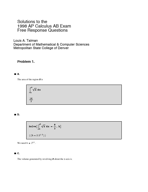
Solutions to the1998 AP Calculus AB ExamFree Response QuestionsLouis A. TalmanDepartment of Mathematical & Computer Sciences Metropolitan State College of DenverProblem 1.‡a.The area of the region R is‡b.We need h=2.‡c.The volume generated by revolving R about the x-axis is‡d.We need k =2 2.Problem 2‡a.lim x Ø-¶2x ‰2 x =lim x Ø-¶2 x ÅÅÅÅÅÅÅÅÅÅÅʼn-2 x . L'Hôpital's Rule is applicable to the latter expression. Thus,lim x Ø-¶2 x ÅÅÅÅÅÅÅÅÅÅÅʼn-2 x =lim x Ø-¶2ÅÅÅÅÅÅÅÅÅÅÅÅÅÅÅÅÅÅ-2 ‰-2 x=0.‡b.If f @x D =2x ‰2 x , then f '@x D =H 2+4x L ‰2 x . Consequently, f '@x D =0 only when x =-1ÅÅÅÅ2. Now (by part a, above)lim x Ø-¶f @x D =0, while lim x ضf @x D =¶. Consequently there are numbers x 1 and x 2, x 1<-1ÅÅÅÅÅÅÅÅ2<x 2, such that x §x 1implies that f @x D ¥-1ÅÅÅÅÅÅÅÅÅ100>f @-1ê2D =-‰-1 and x 2§x implies that f @x D ¥-1ÅÅÅÅÅÅÅÅÅ100>f @-1ê2D . But f must have an absolute minimum in the interva l @x 1,x 2D , and it cannot be located at either x 1 or x 2. Because x =-1ê2 is the onlycritical point in this interval, it must give the absolute minimum for f @x D when x 1§x §x 2, and therefore for -¶<x <¶.‡c.By the observations we have made in part b. above, the range of f is @-‰-1,¶L .‡d.Let us assume, for the moment, that b >0. Then, arguing as we have in parts a. and b. above, we find that f @x D =b x ‰b x has an absolute minimum at x =-1ÅÅÅÅb . This minimum value is f @-1ÅÅÅÅÅÅÅÅb D =-e -1, which is independent of b . If b <0, we obtain the same result after the change of variables u =-x , which amounts to a reflection about the y -axis.Problem 3.The following unpleasant syntax assigns the values given in the table to the function v .‡a.Acceleration is the derivative of velocity, so acceleration is positive at each point where the tangent line to the graph of the velocity function has positive slope. From the picture given, we find that acceleration is positive on the intervals @0,35L and H 45,50D .‡b.Taking a @t D , as the acceleration, average acceleration is 1ÅÅÅÅÅÅ50 Ÿ050a @t D …t =1ÅÅÅÅÅÅ50 H v @50D -v@0DL =1ÅÅÅÅÅÅ50 H 72-0L =36ÅÅÅÅÅÅ25 ft êsec 2.‡c.The acceleration a @40D is approximately v @45D -v @35D ÅÅÅÅÅÅÅÅÅÅÅÅÅÅÅÅÅÅÅÅÅÅÅÅÅÅ10, or (This is in feet êsec .)‡d.The required approximation is:The integral measures, in feet, distance traveled during the time interval 0§t §50.Problem 4‡a.At the point H 1,f @1DL , the slope is 3H 1L 2+1ÅÅÅÅÅÅÅÅÅÅÅÅÅÅÅÅÅÅÅ2f @1D =1ÅÅÅÅ2.‡b.The line tangent to y =f @x D at H 1,f @1DL has equation y =4+1ÅÅÅÅ2 H x -1L . Consequently, f @1.2D is approximately 4+1ÅÅÅÅ2 H 0.2L =41ÅÅÅÅÅÅ10.‡c.From f '@x D =3x 2+1ÅÅÅÅÅÅÅÅÅÅÅÅÅÅÅÅÅ2f @x D , together with f @1D =4, we have 2 Ÿ1x f @t D f '@t D …t =Ÿ1xH 3t 2+1L …t , or 2 Ÿ4f @x D u …u =Ÿ1x H 3t 2+1L …t . Thus, f @x D 2-16=x 3+x -2, or f @x D =è!!!!!!!!!!!!!!!!!!!!!!!!!x 3+x +14. (We have chosen the positivesquare root because f @1D =4>0.)‡d.f @1.2D is given byProblem 5‡a.‡b.Average temperature is1ÅÅÅÅÅÅÅÅÅÅÅÅÅ14-6 Ÿ614F @t D …t :To the nearest degree, this is 87 degrees.‡c.The air conditioner ran when 5.231§t§18.769.‡d.The approximate total cost is 0.05Ÿa b H2-10Cos@p tÅÅÅÅÅÅ12DL …t, or To the nearest cent, this is $5.10.Problem 6‡a.If 2y3+6x2y-12x2+6y=1, then, differentiating implicitly with respect to x while treating y as a function of x, we obtain 6y2y'+12x y+6x2y'-24x+6y'=0. Hence,H6y2+6x2+6L y'=24x-12x y, or y'=H4x-2x y LêH x2+y2+1L.‡b.Tangent lines are horizontal where y'=0. This can happen, according to part a., above, only where 4x-2x y=0, from which we conclude that x=0 or that y=2. If x=0, then from 2y3+6x2y-12x2+6y=1 we conclude that 2y3+6y=1, and we thus have, approximately,An equation for the line tangent to the curve at the corresponding point is y=0.166 (approximately).If y=2, then 16+12x2-12x2+12=1, or 28=1, so there are no horizontal tangent lines where y=2.‡c.At the point where the line through the origin with slope -1 is tangent to the curve, we must have y=-x, because that is the equation of the line in question and the point of tangency lies on that line. Hence -2x3-6x3-12x2-6x=1, or 8x3+12x2+6x+1=0. Equivalently, H2x+1L3=0, so that the only root ofthis equation is x=-1ÅÅÅÅÅÅÅÅ2. Because y=-x at the point in question , y=1ÅÅÅÅ2. The coordinates of the point are H-1ÅÅÅÅ2,1ÅÅÅÅ2L.。

Draft:Deep Learning in Neural Networks:An OverviewTechnical Report IDSIA-03-14/arXiv:1404.7828(v1.5)[cs.NE]J¨u rgen SchmidhuberThe Swiss AI Lab IDSIAIstituto Dalle Molle di Studi sull’Intelligenza ArtificialeUniversity of Lugano&SUPSIGalleria2,6928Manno-LuganoSwitzerland15May2014AbstractIn recent years,deep artificial neural networks(including recurrent ones)have won numerous con-tests in pattern recognition and machine learning.This historical survey compactly summarises relevantwork,much of it from the previous millennium.Shallow and deep learners are distinguished by thedepth of their credit assignment paths,which are chains of possibly learnable,causal links between ac-tions and effects.I review deep supervised learning(also recapitulating the history of backpropagation),unsupervised learning,reinforcement learning&evolutionary computation,and indirect search for shortprograms encoding deep and large networks.PDF of earlier draft(v1):http://www.idsia.ch/∼juergen/DeepLearning30April2014.pdfLATEX source:http://www.idsia.ch/∼juergen/DeepLearning30April2014.texComplete BIBTEXfile:http://www.idsia.ch/∼juergen/bib.bibPrefaceThis is the draft of an invited Deep Learning(DL)overview.One of its goals is to assign credit to those who contributed to the present state of the art.I acknowledge the limitations of attempting to achieve this goal.The DL research community itself may be viewed as a continually evolving,deep network of scientists who have influenced each other in complex ways.Starting from recent DL results,I tried to trace back the origins of relevant ideas through the past half century and beyond,sometimes using“local search”to follow citations of citations backwards in time.Since not all DL publications properly acknowledge earlier relevant work,additional global search strategies were employed,aided by consulting numerous neural network experts.As a result,the present draft mostly consists of references(about800entries so far).Nevertheless,through an expert selection bias I may have missed important work.A related bias was surely introduced by my special familiarity with the work of my own DL research group in the past quarter-century.For these reasons,the present draft should be viewed as merely a snapshot of an ongoing credit assignment process.To help improve it,please do not hesitate to send corrections and suggestions to juergen@idsia.ch.Contents1Introduction to Deep Learning(DL)in Neural Networks(NNs)3 2Event-Oriented Notation for Activation Spreading in FNNs/RNNs3 3Depth of Credit Assignment Paths(CAPs)and of Problems4 4Recurring Themes of Deep Learning54.1Dynamic Programming(DP)for DL (5)4.2Unsupervised Learning(UL)Facilitating Supervised Learning(SL)and RL (6)4.3Occam’s Razor:Compression and Minimum Description Length(MDL) (6)4.4Learning Hierarchical Representations Through Deep SL,UL,RL (6)4.5Fast Graphics Processing Units(GPUs)for DL in NNs (6)5Supervised NNs,Some Helped by Unsupervised NNs75.11940s and Earlier (7)5.2Around1960:More Neurobiological Inspiration for DL (7)5.31965:Deep Networks Based on the Group Method of Data Handling(GMDH) (8)5.41979:Convolution+Weight Replication+Winner-Take-All(WTA) (8)5.51960-1981and Beyond:Development of Backpropagation(BP)for NNs (8)5.5.1BP for Weight-Sharing Feedforward NNs(FNNs)and Recurrent NNs(RNNs)..95.6Late1980s-2000:Numerous Improvements of NNs (9)5.6.1Ideas for Dealing with Long Time Lags and Deep CAPs (10)5.6.2Better BP Through Advanced Gradient Descent (10)5.6.3Discovering Low-Complexity,Problem-Solving NNs (11)5.6.4Potential Benefits of UL for SL (11)5.71987:UL Through Autoencoder(AE)Hierarchies (12)5.81989:BP for Convolutional NNs(CNNs) (13)5.91991:Fundamental Deep Learning Problem of Gradient Descent (13)5.101991:UL-Based History Compression Through a Deep Hierarchy of RNNs (14)5.111992:Max-Pooling(MP):Towards MPCNNs (14)5.121994:Contest-Winning Not So Deep NNs (15)5.131995:Supervised Recurrent Very Deep Learner(LSTM RNN) (15)5.142003:More Contest-Winning/Record-Setting,Often Not So Deep NNs (16)5.152006/7:Deep Belief Networks(DBNs)&AE Stacks Fine-Tuned by BP (17)5.162006/7:Improved CNNs/GPU-CNNs/BP-Trained MPCNNs (17)5.172009:First Official Competitions Won by RNNs,and with MPCNNs (18)5.182010:Plain Backprop(+Distortions)on GPU Yields Excellent Results (18)5.192011:MPCNNs on GPU Achieve Superhuman Vision Performance (18)5.202011:Hessian-Free Optimization for RNNs (19)5.212012:First Contests Won on ImageNet&Object Detection&Segmentation (19)5.222013-:More Contests and Benchmark Records (20)5.22.1Currently Successful Supervised Techniques:LSTM RNNs/GPU-MPCNNs (21)5.23Recent Tricks for Improving SL Deep NNs(Compare Sec.5.6.2,5.6.3) (21)5.24Consequences for Neuroscience (22)5.25DL with Spiking Neurons? (22)6DL in FNNs and RNNs for Reinforcement Learning(RL)236.1RL Through NN World Models Yields RNNs With Deep CAPs (23)6.2Deep FNNs for Traditional RL and Markov Decision Processes(MDPs) (24)6.3Deep RL RNNs for Partially Observable MDPs(POMDPs) (24)6.4RL Facilitated by Deep UL in FNNs and RNNs (25)6.5Deep Hierarchical RL(HRL)and Subgoal Learning with FNNs and RNNs (25)6.6Deep RL by Direct NN Search/Policy Gradients/Evolution (25)6.7Deep RL by Indirect Policy Search/Compressed NN Search (26)6.8Universal RL (27)7Conclusion271Introduction to Deep Learning(DL)in Neural Networks(NNs) Which modifiable components of a learning system are responsible for its success or failure?What changes to them improve performance?This has been called the fundamental credit assignment problem(Minsky, 1963).There are general credit assignment methods for universal problem solvers that are time-optimal in various theoretical senses(Sec.6.8).The present survey,however,will focus on the narrower,but now commercially important,subfield of Deep Learning(DL)in Artificial Neural Networks(NNs).We are interested in accurate credit assignment across possibly many,often nonlinear,computational stages of NNs.Shallow NN-like models have been around for many decades if not centuries(Sec.5.1).Models with several successive nonlinear layers of neurons date back at least to the1960s(Sec.5.3)and1970s(Sec.5.5). An efficient gradient descent method for teacher-based Supervised Learning(SL)in discrete,differentiable networks of arbitrary depth called backpropagation(BP)was developed in the1960s and1970s,and ap-plied to NNs in1981(Sec.5.5).BP-based training of deep NNs with many layers,however,had been found to be difficult in practice by the late1980s(Sec.5.6),and had become an explicit research subject by the early1990s(Sec.5.9).DL became practically feasible to some extent through the help of Unsupervised Learning(UL)(e.g.,Sec.5.10,5.15).The1990s and2000s also saw many improvements of purely super-vised DL(Sec.5).In the new millennium,deep NNs havefinally attracted wide-spread attention,mainly by outperforming alternative machine learning methods such as kernel machines(Vapnik,1995;Sch¨o lkopf et al.,1998)in numerous important applications.In fact,supervised deep NNs have won numerous of-ficial international pattern recognition competitions(e.g.,Sec.5.17,5.19,5.21,5.22),achieving thefirst superhuman visual pattern recognition results in limited domains(Sec.5.19).Deep NNs also have become relevant for the more generalfield of Reinforcement Learning(RL)where there is no supervising teacher (Sec.6).Both feedforward(acyclic)NNs(FNNs)and recurrent(cyclic)NNs(RNNs)have won contests(Sec.5.12,5.14,5.17,5.19,5.21,5.22).In a sense,RNNs are the deepest of all NNs(Sec.3)—they are general computers more powerful than FNNs,and can in principle create and process memories of ar-bitrary sequences of input patterns(e.g.,Siegelmann and Sontag,1991;Schmidhuber,1990a).Unlike traditional methods for automatic sequential program synthesis(e.g.,Waldinger and Lee,1969;Balzer, 1985;Soloway,1986;Deville and Lau,1994),RNNs can learn programs that mix sequential and parallel information processing in a natural and efficient way,exploiting the massive parallelism viewed as crucial for sustaining the rapid decline of computation cost observed over the past75years.The rest of this paper is structured as follows.Sec.2introduces a compact,event-oriented notation that is simple yet general enough to accommodate both FNNs and RNNs.Sec.3introduces the concept of Credit Assignment Paths(CAPs)to measure whether learning in a given NN application is of the deep or shallow type.Sec.4lists recurring themes of DL in SL,UL,and RL.Sec.5focuses on SL and UL,and on how UL can facilitate SL,although pure SL has become dominant in recent competitions(Sec.5.17-5.22). Sec.5is arranged in a historical timeline format with subsections on important inspirations and technical contributions.Sec.6on deep RL discusses traditional Dynamic Programming(DP)-based RL combined with gradient-based search techniques for SL or UL in deep NNs,as well as general methods for direct and indirect search in the weight space of deep FNNs and RNNs,including successful policy gradient and evolutionary methods.2Event-Oriented Notation for Activation Spreading in FNNs/RNNs Throughout this paper,let i,j,k,t,p,q,r denote positive integer variables assuming ranges implicit in the given contexts.Let n,m,T denote positive integer constants.An NN’s topology may change over time(e.g.,Fahlman,1991;Ring,1991;Weng et al.,1992;Fritzke, 1994).At any given moment,it can be described as afinite subset of units(or nodes or neurons)N= {u1,u2,...,}and afinite set H⊆N×N of directed edges or connections between nodes.FNNs are acyclic graphs,RNNs cyclic.Thefirst(input)layer is the set of input units,a subset of N.In FNNs,the k-th layer(k>1)is the set of all nodes u∈N such that there is an edge path of length k−1(but no longer path)between some input unit and u.There may be shortcut connections between distant layers.The NN’s behavior or program is determined by a set of real-valued,possibly modifiable,parameters or weights w i(i=1,...,n).We now focus on a singlefinite episode or epoch of information processing and activation spreading,without learning through weight changes.The following slightly unconventional notation is designed to compactly describe what is happening during the runtime of the system.During an episode,there is a partially causal sequence x t(t=1,...,T)of real values that I call events.Each x t is either an input set by the environment,or the activation of a unit that may directly depend on other x k(k<t)through a current NN topology-dependent set in t of indices k representing incoming causal connections or links.Let the function v encode topology information and map such event index pairs(k,t)to weight indices.For example,in the non-input case we may have x t=f t(net t)with real-valued net t= k∈in t x k w v(k,t)(additive case)or net t= k∈in t x k w v(k,t)(multiplicative case), where f t is a typically nonlinear real-valued activation function such as tanh.In many recent competition-winning NNs(Sec.5.19,5.21,5.22)there also are events of the type x t=max k∈int (x k);some networktypes may also use complex polynomial activation functions(Sec.5.3).x t may directly affect certain x k(k>t)through outgoing connections or links represented through a current set out t of indices k with t∈in k.Some non-input events are called output events.Note that many of the x t may refer to different,time-varying activations of the same unit in sequence-processing RNNs(e.g.,Williams,1989,“unfolding in time”),or also in FNNs sequentially exposed to time-varying input patterns of a large training set encoded as input events.During an episode,the same weight may get reused over and over again in topology-dependent ways,e.g.,in RNNs,or in convolutional NNs(Sec.5.4,5.8).I call this weight sharing across space and/or time.Weight sharing may greatly reduce the NN’s descriptive complexity,which is the number of bits of information required to describe the NN (Sec.4.3).In Supervised Learning(SL),certain NN output events x t may be associated with teacher-given,real-valued labels or targets d t yielding errors e t,e.g.,e t=1/2(x t−d t)2.A typical goal of supervised NN training is tofind weights that yield episodes with small total error E,the sum of all such e t.The hope is that the NN will generalize well in later episodes,causing only small errors on previously unseen sequences of input events.Many alternative error functions for SL and UL are possible.SL assumes that input events are independent of earlier output events(which may affect the environ-ment through actions causing subsequent perceptions).This assumption does not hold in the broaderfields of Sequential Decision Making and Reinforcement Learning(RL)(Kaelbling et al.,1996;Sutton and Barto, 1998;Hutter,2005)(Sec.6).In RL,some of the input events may encode real-valued reward signals given by the environment,and a typical goal is tofind weights that yield episodes with a high sum of reward signals,through sequences of appropriate output actions.Sec.5.5will use the notation above to compactly describe a central algorithm of DL,namely,back-propagation(BP)for supervised weight-sharing FNNs and RNNs.(FNNs may be viewed as RNNs with certainfixed zero weights.)Sec.6will address the more general RL case.3Depth of Credit Assignment Paths(CAPs)and of ProblemsTo measure whether credit assignment in a given NN application is of the deep or shallow type,I introduce the concept of Credit Assignment Paths or CAPs,which are chains of possibly causal links between events.Let usfirst focus on SL.Consider two events x p and x q(1≤p<q≤T).Depending on the appli-cation,they may have a Potential Direct Causal Connection(PDCC)expressed by the Boolean predicate pdcc(p,q),which is true if and only if p∈in q.Then the2-element list(p,q)is defined to be a CAP from p to q(a minimal one).A learning algorithm may be allowed to change w v(p,q)to improve performance in future episodes.More general,possibly indirect,Potential Causal Connections(PCC)are expressed by the recursively defined Boolean predicate pcc(p,q),which in the SL case is true only if pdcc(p,q),or if pcc(p,k)for some k and pdcc(k,q).In the latter case,appending q to any CAP from p to k yields a CAP from p to q(this is a recursive definition,too).The set of such CAPs may be large but isfinite.Note that the same weight may affect many different PDCCs between successive events listed by a given CAP,e.g.,in the case of RNNs, or weight-sharing FNNs.Suppose a CAP has the form(...,k,t,...,q),where k and t(possibly t=q)are thefirst successive elements with modifiable w v(k,t).Then the length of the suffix list(t,...,q)is called the CAP’s depth (which is0if there are no modifiable links at all).This depth limits how far backwards credit assignment can move down the causal chain tofind a modifiable weight.1Suppose an episode and its event sequence x1,...,x T satisfy a computable criterion used to decide whether a given problem has been solved(e.g.,total error E below some threshold).Then the set of used weights is called a solution to the problem,and the depth of the deepest CAP within the sequence is called the solution’s depth.There may be other solutions(yielding different event sequences)with different depths.Given somefixed NN topology,the smallest depth of any solution is called the problem’s depth.Sometimes we also speak of the depth of an architecture:SL FNNs withfixed topology imply a problem-independent maximal problem depth bounded by the number of non-input layers.Certain SL RNNs withfixed weights for all connections except those to output units(Jaeger,2001;Maass et al.,2002; Jaeger,2004;Schrauwen et al.,2007)have a maximal problem depth of1,because only thefinal links in the corresponding CAPs are modifiable.In general,however,RNNs may learn to solve problems of potentially unlimited depth.Note that the definitions above are solely based on the depths of causal chains,and agnostic of the temporal distance between events.For example,shallow FNNs perceiving large“time windows”of in-put events may correctly classify long input sequences through appropriate output events,and thus solve shallow problems involving long time lags between relevant events.At which problem depth does Shallow Learning end,and Deep Learning begin?Discussions with DL experts have not yet yielded a conclusive response to this question.Instead of committing myself to a precise answer,let me just define for the purposes of this overview:problems of depth>10require Very Deep Learning.The difficulty of a problem may have little to do with its depth.Some NNs can quickly learn to solve certain deep problems,e.g.,through random weight guessing(Sec.5.9)or other types of direct search (Sec.6.6)or indirect search(Sec.6.7)in weight space,or through training an NNfirst on shallow problems whose solutions may then generalize to deep problems,or through collapsing sequences of(non)linear operations into a single(non)linear operation—but see an analysis of non-trivial aspects of deep linear networks(Baldi and Hornik,1994,Section B).In general,however,finding an NN that precisely models a given training set is an NP-complete problem(Judd,1990;Blum and Rivest,1992),also in the case of deep NNs(S´ıma,1994;de Souto et al.,1999;Windisch,2005);compare a survey of negative results(S´ıma, 2002,Section1).Above we have focused on SL.In the more general case of RL in unknown environments,pcc(p,q) is also true if x p is an output event and x q any later input event—any action may affect the environment and thus any later perception.(In the real world,the environment may even influence non-input events computed on a physical hardware entangled with the entire universe,but this is ignored here.)It is possible to model and replace such unmodifiable environmental PCCs through a part of the NN that has already learned to predict(through some of its units)input events(including reward signals)from former input events and actions(Sec.6.1).Its weights are frozen,but can help to assign credit to other,still modifiable weights used to compute actions(Sec.6.1).This approach may lead to very deep CAPs though.Some DL research is about automatically rephrasing problems such that their depth is reduced(Sec.4). In particular,sometimes UL is used to make SL problems less deep,e.g.,Sec.5.10.Often Dynamic Programming(Sec.4.1)is used to facilitate certain traditional RL problems,e.g.,Sec.6.2.Sec.5focuses on CAPs for SL,Sec.6on the more complex case of RL.4Recurring Themes of Deep Learning4.1Dynamic Programming(DP)for DLOne recurring theme of DL is Dynamic Programming(DP)(Bellman,1957),which can help to facili-tate credit assignment under certain assumptions.For example,in SL NNs,backpropagation itself can 1An alternative would be to count only modifiable links when measuring depth.In many typical NN applications this would not make a difference,but in some it would,e.g.,Sec.6.1.be viewed as a DP-derived method(Sec.5.5).In traditional RL based on strong Markovian assumptions, DP-derived methods can help to greatly reduce problem depth(Sec.6.2).DP algorithms are also essen-tial for systems that combine concepts of NNs and graphical models,such as Hidden Markov Models (HMMs)(Stratonovich,1960;Baum and Petrie,1966)and Expectation Maximization(EM)(Dempster et al.,1977),e.g.,(Bottou,1991;Bengio,1991;Bourlard and Morgan,1994;Baldi and Chauvin,1996; Jordan and Sejnowski,2001;Bishop,2006;Poon and Domingos,2011;Dahl et al.,2012;Hinton et al., 2012a).4.2Unsupervised Learning(UL)Facilitating Supervised Learning(SL)and RL Another recurring theme is how UL can facilitate both SL(Sec.5)and RL(Sec.6).UL(Sec.5.6.4) is normally used to encode raw incoming data such as video or speech streams in a form that is more convenient for subsequent goal-directed learning.In particular,codes that describe the original data in a less redundant or more compact way can be fed into SL(Sec.5.10,5.15)or RL machines(Sec.6.4),whose search spaces may thus become smaller(and whose CAPs shallower)than those necessary for dealing with the raw data.UL is closely connected to the topics of regularization and compression(Sec.4.3,5.6.3). 4.3Occam’s Razor:Compression and Minimum Description Length(MDL) Occam’s razor favors simple solutions over complex ones.Given some programming language,the prin-ciple of Minimum Description Length(MDL)can be used to measure the complexity of a solution candi-date by the length of the shortest program that computes it(e.g.,Solomonoff,1964;Kolmogorov,1965b; Chaitin,1966;Wallace and Boulton,1968;Levin,1973a;Rissanen,1986;Blumer et al.,1987;Li and Vit´a nyi,1997;Gr¨u nwald et al.,2005).Some methods explicitly take into account program runtime(Al-lender,1992;Watanabe,1992;Schmidhuber,2002,1995);many consider only programs with constant runtime,written in non-universal programming languages(e.g.,Rissanen,1986;Hinton and van Camp, 1993).In the NN case,the MDL principle suggests that low NN weight complexity corresponds to high NN probability in the Bayesian view(e.g.,MacKay,1992;Buntine and Weigend,1991;De Freitas,2003), and to high generalization performance(e.g.,Baum and Haussler,1989),without overfitting the training data.Many methods have been proposed for regularizing NNs,that is,searching for solution-computing, low-complexity SL NNs(Sec.5.6.3)and RL NNs(Sec.6.7).This is closely related to certain UL methods (Sec.4.2,5.6.4).4.4Learning Hierarchical Representations Through Deep SL,UL,RLMany methods of Good Old-Fashioned Artificial Intelligence(GOFAI)(Nilsson,1980)as well as more recent approaches to AI(Russell et al.,1995)and Machine Learning(Mitchell,1997)learn hierarchies of more and more abstract data representations.For example,certain methods of syntactic pattern recog-nition(Fu,1977)such as grammar induction discover hierarchies of formal rules to model observations. The partially(un)supervised Automated Mathematician/EURISKO(Lenat,1983;Lenat and Brown,1984) continually learns concepts by combining previously learnt concepts.Such hierarchical representation learning(Ring,1994;Bengio et al.,2013;Deng and Yu,2014)is also a recurring theme of DL NNs for SL (Sec.5),UL-aided SL(Sec.5.7,5.10,5.15),and hierarchical RL(Sec.6.5).Often,abstract hierarchical representations are natural by-products of data compression(Sec.4.3),e.g.,Sec.5.10.4.5Fast Graphics Processing Units(GPUs)for DL in NNsWhile the previous millennium saw several attempts at creating fast NN-specific hardware(e.g.,Jackel et al.,1990;Faggin,1992;Ramacher et al.,1993;Widrow et al.,1994;Heemskerk,1995;Korkin et al., 1997;Urlbe,1999),and at exploiting standard hardware(e.g.,Anguita et al.,1994;Muller et al.,1995; Anguita and Gomes,1996),the new millennium brought a DL breakthrough in form of cheap,multi-processor graphics cards or GPUs.GPUs are widely used for video games,a huge and competitive market that has driven down hardware prices.GPUs excel at fast matrix and vector multiplications required not only for convincing virtual realities but also for NN training,where they can speed up learning by a factorof50and more.Some of the GPU-based FNN implementations(Sec.5.16-5.19)have greatly contributed to recent successes in contests for pattern recognition(Sec.5.19-5.22),image segmentation(Sec.5.21), and object detection(Sec.5.21-5.22).5Supervised NNs,Some Helped by Unsupervised NNsThe main focus of current practical applications is on Supervised Learning(SL),which has dominated re-cent pattern recognition contests(Sec.5.17-5.22).Several methods,however,use additional Unsupervised Learning(UL)to facilitate SL(Sec.5.7,5.10,5.15).It does make sense to treat SL and UL in the same section:often gradient-based methods,such as BP(Sec.5.5.1),are used to optimize objective functions of both UL and SL,and the boundary between SL and UL may blur,for example,when it comes to time series prediction and sequence classification,e.g.,Sec.5.10,5.12.A historical timeline format will help to arrange subsections on important inspirations and techni-cal contributions(although such a subsection may span a time interval of many years).Sec.5.1briefly mentions early,shallow NN models since the1940s,Sec.5.2additional early neurobiological inspiration relevant for modern Deep Learning(DL).Sec.5.3is about GMDH networks(since1965),perhaps thefirst (feedforward)DL systems.Sec.5.4is about the relatively deep Neocognitron NN(1979)which is similar to certain modern deep FNN architectures,as it combines convolutional NNs(CNNs),weight pattern repli-cation,and winner-take-all(WTA)mechanisms.Sec.5.5uses the notation of Sec.2to compactly describe a central algorithm of DL,namely,backpropagation(BP)for supervised weight-sharing FNNs and RNNs. It also summarizes the history of BP1960-1981and beyond.Sec.5.6describes problems encountered in the late1980s with BP for deep NNs,and mentions several ideas from the previous millennium to overcome them.Sec.5.7discusses afirst hierarchical stack of coupled UL-based Autoencoders(AEs)—this concept resurfaced in the new millennium(Sec.5.15).Sec.5.8is about applying BP to CNNs,which is important for today’s DL applications.Sec.5.9explains BP’s Fundamental DL Problem(of vanishing/exploding gradients)discovered in1991.Sec.5.10explains how a deep RNN stack of1991(the History Compressor) pre-trained by UL helped to solve previously unlearnable DL benchmarks requiring Credit Assignment Paths(CAPs,Sec.3)of depth1000and more.Sec.5.11discusses a particular WTA method called Max-Pooling(MP)important in today’s DL FNNs.Sec.5.12mentions afirst important contest won by SL NNs in1994.Sec.5.13describes a purely supervised DL RNN(Long Short-Term Memory,LSTM)for problems of depth1000and more.Sec.5.14mentions an early contest of2003won by an ensemble of shallow NNs, as well as good pattern recognition results with CNNs and LSTM RNNs(2003).Sec.5.15is mostly about Deep Belief Networks(DBNs,2006)and related stacks of Autoencoders(AEs,Sec.5.7)pre-trained by UL to facilitate BP-based SL.Sec.5.16mentions thefirst BP-trained MPCNNs(2007)and GPU-CNNs(2006). Sec.5.17-5.22focus on official competitions with secret test sets won by(mostly purely supervised)DL NNs since2009,in sequence recognition,image classification,image segmentation,and object detection. Many RNN results depended on LSTM(Sec.5.13);many FNN results depended on GPU-based FNN code developed since2004(Sec.5.16,5.17,5.18,5.19),in particular,GPU-MPCNNs(Sec.5.19).5.11940s and EarlierNN research started in the1940s(e.g.,McCulloch and Pitts,1943;Hebb,1949);compare also later work on learning NNs(Rosenblatt,1958,1962;Widrow and Hoff,1962;Grossberg,1969;Kohonen,1972; von der Malsburg,1973;Narendra and Thathatchar,1974;Willshaw and von der Malsburg,1976;Palm, 1980;Hopfield,1982).In a sense NNs have been around even longer,since early supervised NNs were essentially variants of linear regression methods going back at least to the early1800s(e.g.,Legendre, 1805;Gauss,1809,1821).Early NNs had a maximal CAP depth of1(Sec.3).5.2Around1960:More Neurobiological Inspiration for DLSimple cells and complex cells were found in the cat’s visual cortex(e.g.,Hubel and Wiesel,1962;Wiesel and Hubel,1959).These cellsfire in response to certain properties of visual sensory inputs,such as theorientation of plex cells exhibit more spatial invariance than simple cells.This inspired later deep NN architectures(Sec.5.4)used in certain modern award-winning Deep Learners(Sec.5.19-5.22).5.31965:Deep Networks Based on the Group Method of Data Handling(GMDH) Networks trained by the Group Method of Data Handling(GMDH)(Ivakhnenko and Lapa,1965; Ivakhnenko et al.,1967;Ivakhnenko,1968,1971)were perhaps thefirst DL systems of the Feedforward Multilayer Perceptron type.The units of GMDH nets may have polynomial activation functions imple-menting Kolmogorov-Gabor polynomials(more general than traditional NN activation functions).Given a training set,layers are incrementally grown and trained by regression analysis,then pruned with the help of a separate validation set(using today’s terminology),where Decision Regularisation is used to weed out superfluous units.The numbers of layers and units per layer can be learned in problem-dependent fashion. This is a good example of hierarchical representation learning(Sec.4.4).There have been numerous ap-plications of GMDH-style networks,e.g.(Ikeda et al.,1976;Farlow,1984;Madala and Ivakhnenko,1994; Ivakhnenko,1995;Kondo,1998;Kord´ık et al.,2003;Witczak et al.,2006;Kondo and Ueno,2008).5.41979:Convolution+Weight Replication+Winner-Take-All(WTA)Apart from deep GMDH networks(Sec.5.3),the Neocognitron(Fukushima,1979,1980,2013a)was per-haps thefirst artificial NN that deserved the attribute deep,and thefirst to incorporate the neurophysiolog-ical insights of Sec.5.2.It introduced convolutional NNs(today often called CNNs or convnets),where the(typically rectangular)receptivefield of a convolutional unit with given weight vector is shifted step by step across a2-dimensional array of input values,such as the pixels of an image.The resulting2D array of subsequent activation events of this unit can then provide inputs to higher-level units,and so on.Due to massive weight replication(Sec.2),relatively few parameters may be necessary to describe the behavior of such a convolutional layer.Competition layers have WTA subsets whose maximally active units are the only ones to adopt non-zero activation values.They essentially“down-sample”the competition layer’s input.This helps to create units whose responses are insensitive to small image shifts(compare Sec.5.2).The Neocognitron is very similar to the architecture of modern,contest-winning,purely super-vised,feedforward,gradient-based Deep Learners with alternating convolutional and competition lay-ers(e.g.,Sec.5.19-5.22).Fukushima,however,did not set the weights by supervised backpropagation (Sec.5.5,5.8),but by local un supervised learning rules(e.g.,Fukushima,2013b),or by pre-wiring.In that sense he did not care for the DL problem(Sec.5.9),although his architecture was comparatively deep indeed.He also used Spatial Averaging(Fukushima,1980,2011)instead of Max-Pooling(MP,Sec.5.11), currently a particularly convenient and popular WTA mechanism.Today’s CNN-based DL machines profita lot from later CNN work(e.g.,LeCun et al.,1989;Ranzato et al.,2007)(Sec.5.8,5.16,5.19).5.51960-1981and Beyond:Development of Backpropagation(BP)for NNsThe minimisation of errors through gradient descent(Hadamard,1908)in the parameter space of com-plex,nonlinear,differentiable,multi-stage,NN-related systems has been discussed at least since the early 1960s(e.g.,Kelley,1960;Bryson,1961;Bryson and Denham,1961;Pontryagin et al.,1961;Dreyfus,1962; Wilkinson,1965;Amari,1967;Bryson and Ho,1969;Director and Rohrer,1969;Griewank,2012),ini-tially within the framework of Euler-LaGrange equations in the Calculus of Variations(e.g.,Euler,1744). Steepest descent in such systems can be performed(Bryson,1961;Kelley,1960;Bryson and Ho,1969)by iterating the ancient chain rule(Leibniz,1676;L’Hˆo pital,1696)in Dynamic Programming(DP)style(Bell-man,1957).A simplified derivation of the method uses the chain rule only(Dreyfus,1962).The methods of the1960s were already efficient in the DP sense.However,they backpropagated derivative information through standard Jacobian matrix calculations from one“layer”to the previous one, explicitly addressing neither direct links across several layers nor potential additional efficiency gains due to network sparsity(but perhaps such enhancements seemed obvious to the authors).。