高宏Chapter 2A

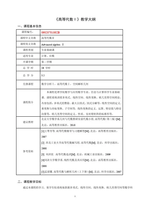
《高等代数Ⅱ》教学大纲
一、课程基本信息
二、课程教学目标
通过本课程的学习，使学生较系统地掌握多项式、线性空间、线性变换、欧几里得空间等数学科
学的基础理论知识和基本计算技巧，学会严密的逻辑推理方法，大力加强学生的归纳、演绎、类比、抽象等能力，为学生学习后继有关课程如近世代数、离散数学、数论等奠定坚实的基础。

三、理论教学内容与要求
四、考核方式
本课程为考试课。

采用期末考试、平时考核相结合的考核方式。

总成绩为100分，其中期末考试成绩占总成绩的70%，平时成绩（包括作业、出勤、课堂表现等）占总成绩的30%。

罗默的《高级宏观经济学》课件一、引言罗默的《高级宏观经济学》是一本在学术界广受推崇的经济学教材，深入浅出地介绍了宏观经济学的基本理论和分析方法。

本书共分为两个部分，第一部分主要讨论宏观经济学的微观基础，包括消费者行为、生产者行为、市场均衡和一般均衡等；第二部分则重点介绍宏观经济学的核心议题，如经济增长、失业、通货膨胀、经济周期等。

本课件旨在帮助读者更好地理解和掌握罗默的《高级宏观经济学》的内容，为宏观经济学的学习和研究提供有益的参考。

二、微观基础1.消费者行为罗默认为，消费者行为是宏观经济学微观基础的重要组成部分。

消费者的目标是实现效用最大化，即在预算约束下，选择一组商品和服务，使得总效用达到最大。

为此，罗默介绍了无差异曲线、预算线等概念，以及如何通过求解拉格朗日函数来找到消费者最优消费组合的方法。

2.生产者行为生产者行为是宏观经济学微观基础的另一个重要组成部分。

罗默认为，生产者的目标是实现利润最大化，即在生产技术、要素价格和市场价格的约束下，选择一组生产要素和产量，使得总利润达到最大。

罗默详细介绍了生产函数、成本函数、利润函数等概念，以及如何通过求解拉格朗日函数来找到生产者最优生产组合的方法。

3.市场均衡和一般均衡罗默认为，市场均衡是宏观经济学的核心概念之一。

市场均衡指的是在某一市场价格下，市场需求等于市场供给。

罗默介绍了如何通过供求曲线来分析市场均衡，以及市场均衡的稳定性条件。

罗默还介绍了一般均衡理论，即在一个包含多个市场和多种商品的体系中，各个市场之间相互影响，形成一个稳定的均衡状态。

三、核心议题1.经济增长罗默认为，经济增长是宏观经济学研究的核心议题之一。

经济增长指的是一个国家或地区在一定时期内，实际产出水平持续提高的过程。

罗默详细介绍了经济增长的源泉，包括技术进步、资本积累、劳动力增长等，并分析了不同增长模型的特点和适用条件。

2.失业罗默认为，失业是宏观经济学的另一个核心议题。

失业指的是劳动力市场上，愿意工作但未能找到工作的人口。

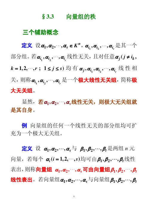
§3.3 向量组的秩三个辅助概念定义 设12,,,ns K ααα∈"，12,,,r i i i αα"αi 是其一个部分组。

若12,,,r i i αα"α线性无关，且对任意(,j k j i α≠1,2,,;1)k r j =≤"s ≤均有12,,,,r j i i i αααα"线性相关，则称12,,,r i i i αα"α是一个极大线性无关组，简称极大无关组。

显然，若12,,,s ααα"线性无关，则极大无关组就是其自身。

例 向量组的任何一个线性无关的部分组均可扩充为一个极大无关组。

定义 设 12,,,s ααα"与 12,,,t ββ"β)是两组n 元 向量，若每个均可由(1,2,,i i s α="12,,,t ββ"β线性 12,,,s ααα"12,,,t 可由向量组βββ" 表出，则称向量组线性表出。

若向量组12,,,s αα"α与向量组12,,,t βββ"可相互线性表出，则称向量组12,,,s ααα"12,,,t 与向量组βββ"12,,,等价，记为{s ααα"}{12,,,t βββ"}≅例 讨论下列向量之间的关系：(1) )1,0(),0,1(21==εε与 )0,0(),0,1(21==αα(2) )1,0(),0,1(21==εε与 )1,2(),2,1(21==ββ性质 向量组的等价具有(1)自反性：{m ααα,...,,21}≅{m ααα,...,,21}；(2)对称性：{s ααα,...,,21}≅{t βββ,...,,21}⇒{t βββ,...,,21}≅{s ααα,...,,21}；(3)传递性：12121212{,,...,}{,,...,}{,,...,}{,,...,}s t t r αααββββββγγγ≅⎫⎬≅⎭⇒{12,,...,s ααα}≅{12,,...,m γγγ}。

罗默《高级宏观经济学》（第3版）第2章 无限期界与世代交叠模型跨考网独家整理最全经济学考研真题，经济学考研课后习题解析资料库，您可以在这里查阅历年经济学考研真题，经济学考研课后习题，经济学考研参考书等内容，更有跨考考研历年辅导的经济学学哥学姐的经济学考研经验，从前辈中获得的经验对初学者来说是宝贵的财富，这或许能帮你少走弯路，躲开一些陷阱。

以下内容为跨考网独家整理，如您还需更多考研资料，可选择经济学一对一在线咨询进行咨询。

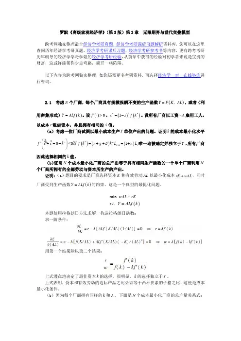
2.1 考虑N 个厂商，每个厂商具有规模报酬不变的生产函数()Y F K AL =，，或者（利用密集形式）()Y ALf k =。

设()·0f '>，()()***1c s f k =-。

设所有厂商以工资wA 雇用工人，以成本r 租借资本，并且拥有相同的A 值。

（a ）考虑一位厂商试图以最小成本生产Y 单位产出的问题。

证明k 的成本最小化水平()()()**1001t t t f c c k cs f k n g k L n L αδ*+⎛⎫"==-=++=+ ⎪⎝⎭＜唯一地被确定并独立于Y ，所有厂商因此选择相同的k 值。

（b ）证明N 个成本最小化厂商的总产出等于具有相同生产函数的一个单个厂商利用N 个厂商所拥有的全部劳动与资本所生产的产出。

证明：（a ）题目的要求是厂商选择资本K 和有效劳动AL 以最小化成本rK wAL +，同时厂商受到生产函数()Y ALf k =的约束。

这是一个典型的最优化问题。

().mi . n s t w Y ALf k AL rK = +本题使用拉格朗日方法求解，构造拉格朗日函数： 求一阶条件：用第一个结果除以第二个结果：上式潜在地决定了最佳资本k 的选择。

很明显，k 的选择独立于Y 。

上式表明，资本和有效劳动的边际产品之比必须等于两种要素的价格之比，这便是成本最小化条件。

（b ）因为每个厂商拥有同样的k 和A ，下面是N 个成本最小化厂商的总产量关系式：单一厂商拥有同样的A 并且选择相同数量的k ，k 的决定独立于Y 的选择。

高等代数教案 The pony was revised in January 2021
高等代数
教案
秦文钊
一、章（节、目）授课计划第页
二、课时教学内容第页
二、课时教学内容第页
一、章（节、目）授课计划第页
二、课时教学内容第页
一、章（节、目）授课计划第页
二、课时教学内容第页
二、课时教学内容第页
二、课时教学内容第页
一、章（节、目）授课计划第页
二、课时教学内容第页
二、课时教学内容第页
一、章（节、目）授课计划第页
二、课时教学内容第页
二、课时教学内容第页
二、课时教学内容第页
一、章（节、目）授课计划第页
二、课时教学内容第页
二、课时教学内容第页
a的代数余子式.称为元素
ij
二、课时教学内容第页
二、课时教学内容第页
一、章（节、目）授课计划第页
二、课时教学内容第页
二、课时教学内容第页
一、章（节、目）授课计划第页
二、课时教学内容第页
二、课时教学内容第页。

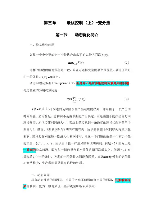
第三章 最优控制（上）-变分法第一节 动态优化简介一、静态优化问题如果一个企业要确定一个最优产出水平x *以最大利润()F x ：0max ()x F x ≥ （1）这样的问题的解通常将是一数，即确定选择变量的单个最优值。

最优值常可由一阶条件()0F x *'=确定。

动态问题是多期（multiperiod ）的，但是并不是有多期的时间就是动态问题．．．．．．．．．．．．．．．．．。

考虑企业的多期决策问题：1max (,)Tt t F t x =∑ （2）(0,1)t x t T = 描述的是每阶段的产出组成的序列，即给出了一个产出的时间路径。

显而易见，总利润不是由单期的产出决定，而是由整个的产出的时间路径确定，所以要使利润最大化，实质上是要找到一条最优的路径（而不是单个期的t x ）。

但由于t 期利润只与t 期的产出有关，所以要在整个时间序列内最大化利润，就只要分别在每一期最大化利润即可，即这一个问题的解是一个有T 个数的集合，1{,}T x x ** 。

所以由于任一产量只影响该期利润，问题（2）实际上是一系列的．．．．静态问题，即在每一期选择当前产量使该期利润最大化。

问题（2）有类似的T 个一阶条件，各期的一阶条件之间没有联系。

在Ramsey 模型的竞争性均衡结构中，生产者问题就具有这样的性质。

二、动态问题具有动态性质的问题是，当前的产出不但影响到当前的利润，还影响到未．．．．．来．的利润。

更为一般地来说，当前决策影响未来决策。

11max (,,).. 0,1Tt t t t F t x x s t x t T-=≥=∑0x 给定或0(0)x x = （3）在问题（3）中，每一期的利润不但取决于当前产量，还与过去的产量有关；换句话说，t 期选择的产量t x 不但影响t 期的利润，还会影响到以后的利润。

注意，上述问题中已指定了0x 。

0x 影响到了以后各期的利润（从而也影响到总利润）。

问题（3）与问题（2）不同，它的最优解的T 个一阶条件不能分别确定，而是要同时确定，也就是我们实际上要“一次性”确定一条最优路径。

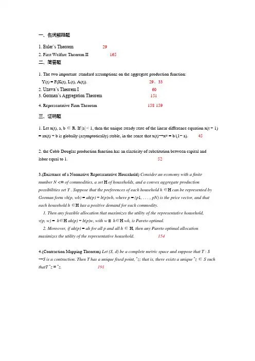
1. Euler’s Theorem292. First Welfare Theorem II 165二、简答题1. The two important standard assumptions on the aggregate production function:Y(t) = F(K(t), L(t), A(t)). 29、332. Uzawa’s Theorem I 603. Gorman’s Aggregation Theorem 1514. Representative Firm Theorem 158-159三、证明题1. Let x(t), a, b ∈ R. If |a| < 1, then the unique steady state of the linear difference equation x(t + 1) = ax(t) + b is globally (asymptotically) stable, in the sense that x(t)→x∗ = b/(1− a). 452.the Cobb-Douglas production function has an elasticity of substitution between capital and labor equal to 1. 523.(Existence of a Normative Representative Household) Consider an economy with a finite number N <∞ of commodities, a set H of households, and a convex aggregate production possibilities set Y . Suppose that the preferences of each household h ∈H can be represented by Gorman form vh(p, wh) = ah(p) + b(p)wh, where p = (p1, . . . , pN) is the price vector, and that each household h ∈H has a positive demand for each commodity.1. Then any feasible allocation that maximizes the utility of the representative household,v(p, w) =_h∈H ah(p) + b(p)w, with w ≡_h∈H wh, is Pareto optimal.2. Moreover, if ah(p) = ah for all p and all h ∈ H, then any Pareto optimal allocation maximizes the utility of the representative household. 1544.(Contraction Mapping Theorem) Let (S, d) be a complete metric space and suppose that T : S→S is a contraction. Then T has a unique fixed point, ˆz; that is, there exists a unique ˆz ∈S such thatT ˆz = ˆz. 1911. Inada Conditions 332. Contraction Mapping and fixed point 191二、简答题1. Types of Neutral Technological Progress 58-592. Uzawa’s Theorem II 633. Debreu-Mantel-Sonnenschein Theorem 1504. Second Welfare Theorem 167三、证明题1. (Euler’s Theorem) Suppose that g :R K+2→R is differentiable in x ∈ R and y ∈ R, with partial derivatives denoted by gx and gy, and is homogeneous of degree m inx and y. Then mg(x, y, z) = gx(x, y, z)x + gy(x, y, z)y for all x ∈ R, y ∈ R, and z ∈ R K.Moreover, gx(x, y, z) and gy(x, y, z) are themselves homogeneous of degree m − 1in x and y. 292.Let g :R→R be differentiable in the neighborhood of the steady state x∗, defined by g(x∗) =x∗,and suppose that__g(x∗)__< 1. Then the steady state x∗ of the nonlinear difference equation x(t + 1) = g(x(t)) is locally (asymptotically) stable. Moreover, if g is continuously differentiable and satisfies __g(x)__< 1 for all x ∈ R, then x∗ is globally(asymptotically) stable. 453 (Uzawa’s Theorem I) Consider a growth model with aggregate production functionY(t) = ˜ F(K(t), L(t), ˜ A(t)),where ˜ F :R2+ × A→R+ and ˜ A(t) ∈ A represents technology at time t (where A is anarbitrary set, e.g., a subset of R N for some natural numberN). Suppose that ˜ F exhibits constant returns to scale in K and L. The aggregate resource constraint is˙ K(t) = Y(t) −C(t) −δK(t ).Suppose that there is a constant growth rate of population, L(t) = exp(nt)L(0), and that there exists T <∞ such that for all t ≥ T , ˙ Y (t)/Y (t) = gY > 0, ˙K (t)/K(t) = gK > 0,and˙C(t)/C(t) = gC > 0. Then1. gY= gK= gC; and2. for any t ≥ T , there exists a functionF :R2+→R+ homogeneous of degree 1 in its two arguments, such that the aggregate production function can be represented asY(t) = F(K(t), A(t)L(t)),where A(t) ∈ R+ and˙ A(t)A(t)= g = gY−n.604. Construct a continuous-time version of the model with finite lives and random deaths (recall(5.12)in the text). In particular suppose that an individual faces a constant (Poisson) flow rate of death equal to ν >0 and has a true discount factor equal to ρ. Show that this individual behaves as if she were infinitely lived with an effective discount factor of ρ + ν. 1791. First Welfare Theorem I 1642. Locally asymptotically stable and globally asymptotically stable 44二、简答题1. The two reasonable microfoundations for the Infinite Planning Horizon 156-1572. Existence of a Normative Representative Household 1543. Why is there such a difference between the representative household and representative firm assumptions? 1594 The five assumptions on Stationary Dynamic Programming Theorems 187-188三、证明题1. Suppose that Assumptions 1 and 2 hold. Then the steady-state equilibrium of the Solow growth model described by the difference equation (2.17) is globally asymptotically stable, and starting from any k(0) > 0, k(t) monotonically converges to k∗. 452. (Uzawa’s Theorem II) Suppose that all hypotheses in Theorem 2.6 are satisfied, so that ˜F :R2+ × A→R+ has a representation of the form F(K(t), A(t)L(t)) withA(t) ∈ R+ and ˙ A(t)/A(t) = g = gY−n (for t ≥ T ). In addition, suppose that factor markets are competitive and that for all t ≥ T , the rental rate satisfies R(t) = R∗(or equivalently,αK(t) = α∗K). Then, denoting the partial derivatives of ˜ F and F with respect to their first two arguments by ˜ FK, ˜ FL, FK, and FL, we have˜ FK(K(t ), L(t), ˜ A(t)) = FK(K(t ), A(t)L(t)) and˜ FL(K(t ), L(t), ˜ A(t)) = A(t)FL(K(t ), A(t)L(t)). (2.43)Moreover, if (2.43) holds and factor markets are competitive, then R(t) = R∗(and αK(t) = α∗K) for all t ≥ T . 633. (FirstWelfare Theorem I) Suppose that (x∗, y∗, p∗) is a competitive equilibrium of economy E ≡ (H, F, U, ω, Y, X, θ) with H finite. Assume that all households arelocally nonsatiated. Then (x∗, y∗) is Pareto optimal. 1644. (Representative Firm Theorem) Consider a competitive production economy with N ∈ N ∪{+∞} commodities and a countable set F of firms, each with a production possibilities set Y f ⊂R N. Let p ∈ R N+ be the price vector in this economy and denote the set of profit-maximizing net supplies of firm f ∈ F by ˆ Y f (p) ⊂Y f (so that for any ˆy f ∈ ˆ Y f (p), we have p . ˆy f ≥ p . yf for all yf ∈Y f ). Then there exists a representative firm with production possibilities set Y ⊂ R N and a set of profit-maximizing net supplies ˆ Y(p) such that for any p ∈ R N+, ˆy ∈ ˆ Y(p) if and only if ˆy =_f ∈Fˆyf for some ˆy f ∈ ˆ Y f (p) for each f ∈ F. 158-159。

Advanced Macroeconomics IInstructor:Luo DaqingAssignment1Note:You may use either English or Chinese to answer the questions.Question1(3points,1point for each part)This question seeks to clarify the concept of expectations,conditional and unconditional.(a)Consider a two-period model where consumption in period t is a random variable denoted C t,for t=0,1.For simplicity,assume that C t can take on two values,c t and c t, for t=0,1.Show that when C t is identically and independently distributed over timeE0(C1)=E[C1].(b)Consider a two-period model where consumption in period t is a random variable denoted C t,for t=0,1.For simplicity,assume that C t can take on two values,c t and c t,for t=0,1.Show thatE[E0(C1)]=E[C1].(c)Consider a three-period model where a consumer seeks to maximize her lifetime expected utilityE02t=0βt u(C t)=u(c0)+β[u(c1)·P r(C1=c1|c0)+u(c1)·P r(C1=c1|c0)] +β2[u(c2)·P r(C2=c2|c0)+u(c2)·P r(C2=c2|c0)]where C1and C2are random variables that can take on only two values,c t and c t,for t=1,2.How would you calculate the conditional probabilities P r(C2=c2|c0)and P r(C2=c2|c0)?Question2(3.5points)Consider an extension of the two-period endowment economy studied in class where agents live for four periods.A representative agent has lifetime expected utilityE1U=ln(c1)+0.96E1ln(c2)+0.962E1ln(c3)+0.963E1ln(c4)where c t denotes consumption in period t.Each agent receives an endowment y t in period t.denote the price of a one-period bond purchased in period t and (a)(0.5pts)Let q Sbtpaying one unit of consumption in period t+1.State(no deviations nor explanations required)an expression relating the price q Sto y1and y2.b1(b)(0.5pts)Let q Mdenote the price of a two-period bond purchased in period t and btpaying one unit of consumption in period t+2.State(no deviations nor explanationsto y1and y3.required)an expression relating the price q Mb1(c)(0.5pts)Let q Ldenote the price of a three-period bond purchased in period t and btpaying one unit of consumption in period t+3.State(no deviations nor explanations required)an expression relating the price q Lto y1and y4.b1(d)(1pts)Consider the following contract.In period1,buyer and seller agree on the following:(1)in period3,the buyer has to pay f units of consumption to the seller;(2)in period4,the seller has to pay1unit of consumption to the buyer.Explain what are the utility costs and benefits to the buyer of signing the above described contract. What is the equation relating the price f to endowments?and (e)(1pts)Using your answer from part(d),derive an expression relating f,q Lb1q Mand briefly explain why this equation has to hold in equilibrium.b1Question3(3.5points)Consider a three-period economy with a large number of identical consumers,firms and banks.Assume the number offirms coincides with the number of consumers and that eachfirm is entirely owned by a consumer with the following utility functionU=ln(c1)+0.95E1ln(c2)+0.952E1ln(c3).A representativefirm considers investing into a new machine.The machine would be bought at price P and installed in period1and would be productive in periods2and3 only.The payoffs generated by the machine in periods2and3are denoted py2and py3, respectively.Assume that consumption is contingent on the state of the economy.More specifically, consumption is equal to1.2when the economy is in a good state and to0.4when the economy is in a bad state.Assume that the economy is in a good state in period1(i.e. c1=1.2).The payoffs generated by the machine are also state contingent.The payoffis0.2in the good state and0.1in the bad state.Finally,the state of the economy evolves independently over time and both states have probability0.5.(a)(0.5pts)Suppose thefirm has the resources necessary to completely cover the purchasing price of the machine in period1.State the Euler equation linking the price of the machine,its payoffs and current and future consumption.Clearly explain your answer in terms of costs and benefits related to such an investment.(b)(0.5pts)Using your answer to part(a),show that the equilibrium price thefirm is willing to pay for the machine is0.4631.From now on,we assume that the market price of the machine is P=0.4631and that thefirm has to borrow to be able to acquire the machine.(c)(0.5pts)Suppose the bank requires thefirm to make a down payment D in period 1and payments of equal amount m in periods2and3.Write the Euler equation linking D,m,the machine’s payoffs and current and future consumption.Clearly explain your answer in terms of costs and benefits related to such an investment.(d)(0.5pts)Using your answer to part(c)and assuming D=0.23,solve for the equilibrium amount m thefirm is willing to pay in periods2and3.(e)(0.5pts)Suppose the bank charges a periodic real interest rate r=0.03and uses the following present-value formulaP=D+m1+r+m(1+r)2to determine m.Again,assuming D=0.23,solve for the amount m the bank will charge afirm borrowing to buy a machine.(f)(1pts)In light of your results,are the market for machines and loans in equilibrium? If not,discuss the adjustments that will take place in the economy to bring the markets to equilibrium.。

第一章 数学预备知识本章讲述若干数学预备知识，包括导数及其应用、静态优化、积分、微分方程、差分方程以及相位图分析等内容。

这些预备性的数学知识对于学习高级宏观经济学是必须的，但是在微观经济学、数理经济学、时间序列分析、高等数学等课程中有详细的讨论，在这里我们只是将与我们后面的学习有关的知识要点罗列在一起并在必要时做出一定的经济解释。

这里的数学知识只是与动态优化相关的部分，对于学习高级宏观经济学必须的其他数学知识并未涉及，特别是时间序列、概率论等知识。

第一节 导数及其应用一、导数有函数()f q π=，导数就是111()()limlim q q q f q q f q d dqq qππ∆→∞∆→∞+∆-∆==∆∆。

导数的经济含义是：边际量、q 变动一单位时π变动的大小、q 对π的变动速率。

二、常用求导公式（1）f b =为常数，0df dbdx dx ==； （2）b 为常数，(())d bf x dfb bf dx dx'==； （3）b 为常数，1bb dx bx dx-=； （4）1(ln )x x'=； （5）()ln x x a a a '=； （6）()x x e e '=； （7）()f g f g '''+=+；（8）()fg f gfg '''=+； （9）2()f f gfg g g ''-'=；（10）链式法则：(),()y f x x g z dy dy dxdz dx dz===【例题1-1】：求下面各题的导数。

（1）32 3y x y x '=⇒= （2）34 3y x y x --'=⇒=-（3）23 25621212(25)z y y x dz d z dy y y x dx dy dx ==+'=⋅=⨯==+（4）()()ax ax ax de de d ax e a dx d ax dx =⋅=⋅练习：求导数[]ln()d ax dx、[]ln ()d x t dt、2(ln )d x dx三、二阶导数二阶导数表示边际量的变化速率，可用如下方式表示：22(),,()d y d dy f x dx dx dx''四、微分22(),[]()y f x dy f dx d f dx d dy d y dx f dx dx f dxdx'=='''''==== 导数是微商。

不变相对风险回避系数效用函数的替代弹性。

考虑一个人，他只存活两期，且其效用函数由（2.46）给出。

令12,P P 代表消费品在这两期的价格，W 代表他一生收入的价值；因此他的预算约束为1122PC P C W +=。

a) 若12,P P 和W 给定，则使他效用最大化的1C 和2C 是多少？b) 两期消费之间的替代弹性为()()1212ln //ln /C C P P -∂∂。

证明：若效用函数由（2.46）式给出，则1C 和2C 之间的替代弹性为1/θ。

答：a) 该效用最大化问题为：st 1122PC P C W += 容易求得其FOC 条件为：()()1/1/12121/C P P C θθρ=+将其代入到约束条件中得到：()()()221/1/21/11/W P C P Pθθθρ-=⎡⎤++⎣⎦()()()()()()1/1/21211/1/211//11/P P W P C P P θθθθθρρ-+=⎡⎤++⎣⎦b) 证明：根据FOC 条件()()1/1/12121/C P P C θθρ=+()()()()()1221ln /1/ln 11/ln /C C P P θρθ⇒=++所以消费的替代弹性为()()1212ln /1ln /C C P P θ∂-=∂。

生产率增长放慢和储蓄。

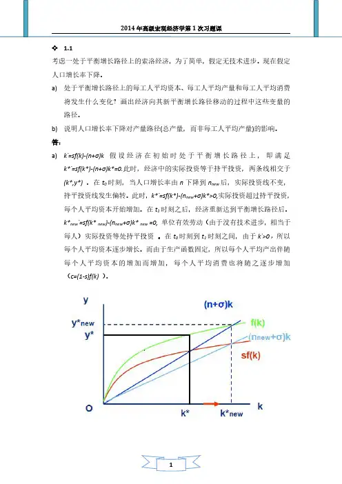
考虑一处于平衡增长路径上的拉姆齐-卡斯-库普曼斯经济，并假定g 有一个永久性的下降。

a) 这如何影响0k= 曲线？ b) 这如何影响0c= 曲线？ c) 在这种变化发生之时，c 如何变动？d) 用一个式子表示g 的一个边际变化对平衡增长路径上的储蓄率的影响。

可否判定这一表达式为正还是为负？e) 若生产函数为柯布-道格拉斯生产函数()f k k α=。

请用,,,,n g ρθα重写上一问的答案。

答：a) 关于资本的欧拉方程为：()()()()()()k t f k t c t n g k t =--+ 。

所以g 的永久性下降会导致0k= 曲线向上移动。

Economics 205C Spring 2010 UCSC C. WalshAdvanced Macroeconomic TheoryEconomics 205CThis course is the third of the three-quarter sequence in macroeconomics for students in the Ph.D. Program in International Economics. The main emphasis will be on new Keynesian models for closed and open economies, optimal monetary policy, and financial frictions.The basic text for the course will be C. E. Walsh, Monetary Theory and Policy (3nd ed., MIT Press, 2010). Required readings are denoted by *. Other readings not listed as required are useful references if you are interested in pursuing a particular topic It is important that you do the required readings before coming to lecture!Your evaluation in this course will be based on an in-class midterm (tentatively scheduled for Monday, May 3rd), a referee report, a three hour final exam, and your participation in class discussions. The final exam is scheduled for Wednesday, June 9 7:30-10:30pm. Exercises and many of the readings will be posted at /~walshc/205Csp10/.My office hours will be Tuesday 9-10am and Wednesday 3:30-4:30 (or by appointment) in 467 E2. My office phone is 9-4082 and my email address is walshc@.I. Nominal frictions, time dependent and state dependent models of price adjustment*Walsh, C. E., Monetary Theory and Policy, 3rd ed. 2009, chapter 6.Nakamura, E. and J. Steinsson, “Five Facts about Prices: An Evaluation of Menu Cost Models,” Quarterly Journal of Economics, 123(4), Nov. 2008, 1415-1464.Klenow, Peter J. and Oleksiy Kryvtsov, “State-Dependent or Time-Dependent Pricing: Does it Matter for Recent U.S. Inflation?” Quarterly Journal of Economics, 123(3), Aug. 2008, 863-904.II. The basic new Keynesian frameworkII. 1 *Walsh, C. E., Monetary Theory and Policy, 3rd ed. 2009, chapter 8, sections 1-3.Woodford, M., Interest and Prices, Princeton University Press, 2003, Chapters 3 and 4.II.2 Linear quadratic toolsLjungqvist and Sargent, Sections 5.1-5.5.Svensson, L. E. O., “Optimization under Commitment and Discretion, the Recursive Saddlepoint Method, and Targeting Rules and Instrument Rules: Lecture Notes,” January 2010, http://people.su.se/~leosven/papers/CommDiscTRIR.pdfII.3 Policy issues*Walsh, C. E., Monetary Theory and Policy, 3rd ed. 2009, chapter 8, sections 4-5.Clarida, R., J. Galí, and M. Gertler, “The Science of Monetary Policy: A New Keynesian Perspective,” Journal of Economic Perspectives, 37(4), 1999, 1661-1707.Chari, V. V., P. J. Kehoe and E. R. McGrattan. 2009. “New Keynesian Models: Not Yet Useful for Policy Analysis,” American Economic Journal Macroeconomics, 1(1): 242-266.II.4 Fiscal policy*Walsh, Monetary Theory and Policy, 3rd ed., 4.1-4.5, 11.1-11.4.*Gali, J., J. Valles, and D. Lopez-Salido, Understanding the effects of government spending on consumption, Journal of the European economic Association March 2007, 5(1): 227-270.Woodford, M., Simple Analytics of the Government Expenditure Multiplier, NBER Working paper 15714, Jan. 2010.III. The open economy*Walsh, Ch. 9, sections 9.4-9.5.*Galí, J. and T. Monacelli, Monetary Policy and Exchange Rate Volatility in a Small Open Economy, Review of Economic Studies, 707-734, 2005.Galí, J. and T. Monacelli, Optimal Monetary and Fiscal Policy in a Currency Union, Journal of International Economics, December 76 (2008), 116-132.IV. Financial factorsIV.1. Interest rates*Walsh, Ch. 10, sections 10.1-10.4Eggertsson, G. B. and M. Woodford. 2003. “The Zero Bound on Interest Rates and Optimal Monetary Policy,” Brookings Papers on Economic Activity, 1, 139-211.Rudebusch, G. D., and T. Wu, "A Macro-Finance Model of the Term Structure, Monetary Policy, and the Economy,” Economic Journal 118, July 2008, 906-926.Ang, A. and M. Piazzesi, “A No-Arbitrage Vector Autoregression of Term Structure Dynamics with Macroeconomic and Latent Variables,” Journal of Monetary Economics, 50,2003, 745-787.Piazzi, M.,IV.2. Market segmentation*Walsh, Ch. 5, section 5.3.Alvarez, F., A. Atkeson, and P. J., Kehoe, “Money, Interest Rates, and Exchange Rates with Endogenously Segmented Markets,” Journal of Political Economy 2002, vol. 110 (1), 73-112.Carlstrom, C. T. and T. S. Fuerst, "Interest Rate Rules vs. Money Growth Rules: A Welfare Comparion in a Cash-in-Advance Economy," Journal of Monetary Economics, 36(2), Nov. 1995, 247-267.IV.3. Imperfect and asymmetric information*Walsh, Ch. 10, sections 10.5—10.6*Akerlof, George A., "The market for `lemons': Quality uncertainty and the market mechanism," Quarterly Journal of Economics, 84(3), Aug. 1970, 488-500.*Gertler, M. and N. Kiyotaki, “Financial Intermediation and Credit Policy in Business Cycle Analysis,” October 2009Diamond, Douglas W., "Banks and liquidity creation: A simple exposition of the Diamond-Dybvig model," Federal Reserve Bank of Richmond Economic Quarterly, 93(2), Spring 2007.Bernanke, B. S. and M. Gertler, "Agency Costs, Net Worth, and Business Fluctuations,"American Economic Review, 79(1), Mar. 1989, 14-31.Carlstrom, C. T., and T. S. Fuerst, "Agency Costs, Net Worth, and Business Fluctuations: A Computable General Equilibrium Analysis," American Economic Review, 87(5), Dec. 1997, 893-910.IV.4. And optimal policyC. T. Carlstrom, T. S. Fuerst and M. Paustian, "Optimal Monetary Policy in a Model with Agency Costs," Aug. 2009.Cúrdia, V. and M. Woodford. 2008. "Credit Frictions and Optimal Monetary Policy," Discussion Papers 0809-02, Columbia University.De Fiore, F. and O. Tristani. 2009. "Optimal Monetary Policy in a Model of the Credit Channel." March.Faia, E. and T. Monacelli. 2007. "Optimal Interest rate Rules, Asset Prices, and Credit Frictions," Journal of Economic Dynamics and Control. 31: 3228-3254.Iacoviello, M. 2005."Housing Prices, Borrowing Constraints, and Monetary Policy in the Business Cycle," American Economic Review 95(3): 739-764.V. Real FrictionsV.1. Informational frictions*Walsh, Ch. 5, section 5.2.Mankiw, N. G. and R. Reis, “Sticky Information versus Sticky Prices: A Proposal to Replace the New Keynesian Phillips Curve,” Quarterly Journal of Economics, 2002, 1295-1328.Mankiw, N. G. and R. Reis,”Imperfect Information and Aggregate Supply," NBER Working Papers 15773, 2010.Mankiw, N. G. and R. Reis,”Sticky Information in General Equilibrium," Journal of the European Economic Association, MIT Press, 2007, vol. 5(2-3), pages 603-613, 04-05.V.2. Variable capital utilization, habit persistence in empirical DSGE modelsChristiano, L. J., M. Eichenbaum, and C. Evans, “Nominal Rigidities and the Dynamic Effects of a Shock to Monetary Policy,” Journal of Political Economy 113(1), Feb. 2005, 1-45.Smets, F. and R. Wouters, “An Estimated Dynamic Stochastic General Equilibrium Model of the Euro Area,” Journal of the European Economic Association, 1(5), 2003, 1123-1175.Smets, F. and R. Wouter, “Shocks and Frictions in US Business Cycles: A Bayesian Approach,” American Economic Review, 97(3), June 2007, 586-606.Adolfsen, M., S. Laséen, J. Lindé, and M. Villani, “Bayesian Estimation of an Open Economy DSGE Model with Incomplete Pass-Through,” Journal of International Economics,72(2), July 2007, 481-511.V.3. UnemploymentSearchMortensen, D. T. and C. A. Pissarides, “Job creation and job destruction in the theory of unemployment,” Review of Economic Studies, 61 (3), July 1994, 397-416.Shimer, Robert, “The Cyclical Behavior of Equilibrium Unemployment and Vacancies,” American Economic Review, 2005, 95(1), 25-49.Walsh, C. E., “Labor market search, sticky prices, and interest rate policies,” Review of Economic Dynamics, 8(4), Oct. 2005, 829-849.Ravenna, F. and C. Walsh, “Welfare-based optimal monetary policy with unemployment and sticky prices: A linear-quadratic framework,” March 2010.。

Lecture 1 The Solow Growth Model Romer(2001), Advanced Macroeconomics, Chapter 1 Blanchard, Olivier J., 2nd edition, Macroeconomics, Prentice Hall曼昆，《宏观经济学》，人民大学，2000年巴罗，萨拉伊马丁，《经济增长》，中国社会科学出版社，2000年Some Basic Facts about Economic Growth Assumptions of One-Sector Growth Models The Dynamics of the ModelThe Impact of a Change in the Saving Rate The Speed of ConvergenceThe Solow Model and the Central Questions of Growth TheoryEmpirical Applications一、Some Basic Facts about EconomicGrowth: the stylized facts of growth 1. Economic growth through deep time(F2)2. The stylized facts✓ 0,>>y L Y （F3）✓ o k L K >> ,(F4)✓ tcons Y K Y K tan ,==(F5)✓ tcons YP YWt cons YP t cons KP tan 1,tan ,tan =-====ρ3. international differences in the standard of living (F6)4. The Solow growth modelThe ultimate objective of research on economic growth is to determine whether there are possibilities for raising overall growth or bringing standards of living in poor countries closer to those in the worldleaders.The Solow model is the starting point for almost all analyses of growth.The principal conclusion of the Solow model is that the accumulation ofphysical capital cannot account for either the vast growth over time in output per person or the cast geographic differences in output per person. The model treats other potential sources of differences in real incomes as either exogenous and thus not explained by the model.( in the case of technological progress) or absent altogether(in the case of positive externalities from capital).二、 Basic assumptions of one-sectorgrowth models1． Input and Output),(t t t t L A K F Y1) Labor-augmenting or Harrod-neutral),(t t t t L K A F Y = capitalaugmenting),(t t t t L K F A Y = Hicks-ueutral2) The ratio of capital to output, K/Y, eventually settles down 3) Constant returns to scale (first-degree homogeneity)✓ The economy is big enough that the gains from specialization have been exhausted.✓ Inputs other than capital, labor, and knowledge are relatively unimportant. 4) intensive form :)()1,(t t k f ALK F ALY y ===✓ The amount of output per unit of effective labor depends only on the quantity of capital per unit of effective labor, and not on the overall size of theeconomy.✓ output per worker)(k Af ALY AL Y ==5) Assumptions 0)0(=f 0,0<''>'f f)(lim )(lim 0='∞='∞→→k f k f k k ( Inada conditions)✓ The path of the economy does not diverge✓ Cobb-Douglas functionαα==kALK k f )()(2． the evolution of the input into production1) Labor and knowledge grow at constant rates:nt L L nL L eL L t tt ntt +=⇔=⇔=00ln )ln(gtL A gA A eA A t tt gtt +=⇔=⇔=00ln )ln(2) Investment and capital formationtt t t t sY S I dtdK dtdK I S G I T S =====+=+t t tK sY Kδ-=三、 The simple dynamics of growth model1． The Harrod-Domar model1) The fixed-coefficients productionfunction⎥⎦⎤⎢⎣⎡αυ=t t t L K Y ,min2) Saving, investment, and the warranted rate of growthυ==s I Y3) Labor force growth:g n Y +=4) The Harrod-Domar condition:υ=+s g n2． The Solow model1) Cobb-Douglas function(F7)kk y ALK AL YK Y k k MPk kMPkkALY y AL K Y )(1)1()(0)(211===υ<-αα=∂∂>α====-α-ααα-α2) The dynamics of kg yLY k f LeK f LeY EY y E K F Y eL E gtgtt t t tg n t +=======+ )()()(),()(0O ne way: actual and break-even investmentk g n k sf k dtdk tt)()(δ++-==0)()(>⇒δ++>kk g n k sf t , k is rising0)()(>⇒δ++<k k g n k sf t , k is falling 0)()(>⇒δ++=k k g n k sf t, k is constant*)(*)(k g n k sf δ++=T he second way: speedk g n k sf k dtdk tt)()(δ++-==)()()ln(δ++-=g n kk sf dt k d t t)(**)(δ++=g n k k sf)()ln(1δ++-=-αg n skdtk d tt)]([)ln()()ln(1δ++-⨯α=α==-ααg n skdtk d dtk dlin dty d tt t t3) the balanced growth path*************)(*k A L K y A L Y y k Y K k L A K Y L A Y k f y t tt t t t t t t t t t t t ======**)(k sgn k f ++δ=nLL g n II CC KK Y Y =>+==== 0)()()()(====ALIAL C AL K AL Yg LIL C L K L Y ====)()()()()]()([)()()),((t t t t t tt t t t t t t k f k k f A k f L K k f A dL L A K F d w '-='-==)()),((t t t t t k f dKL A K F d r '==t t t t t Y K r L w =+tt tt t t L K L k f k k f A K k f L w K r S S ⋅'-⋅'==*)](**)([**)(*)](**)([**)(k f k k f k k f '-⋅'=(constant)The Solow model implies that, regardless of its starting point, the economy converges to a balanced growth path --- a situation where each variable of the model is growing at a constant rate. On the balanced growth path, the growth rate of output per worker is determined solely by the rate of technological progress.四、 The impact of a change in the savingrateThe division of the government ’spurchanses between consumption and investment goods, the division of its revenues between taxed and borrowing, and its tax treatments of saving andinvestment are all likely to affect the fraction of output that is invested.1. the impact on output(F24,F25)A change in the saving rate has a level effect but not a growth effec t: it changes the economy’s balanced growth path, and thus the level of output per worker at any point in time, but it does not affect the growth rate of output per worker in the balanced growth path.In the Solow model only changes in the rate of technological progress have growth effects; all other changes have only level effects .2. saving and consumption (welfare) )()()()1(t t t t k sf k f k f s c -=-=*)(*)(*)(*)(*)()1(*);(**k g n k f k sf k f k f s c s k k δ++-=-=-== sg n s k g n g n s k f s c ∂δ∂δ++-δ'=∂∂),,,(*)](),,,(*([*if )(),,,(*(δ++>δ'g n g n s k f , 0*>∂∂s c if )(),,,(*(δ++<δ'g n g n s k f , 0*<∂∂s c if )(),,,(*(δ++=δ'g n g n s k f ,0*=∂∂s c the golden-rule level of the capital stock: Consumption is at its maximum possible level among balanced growth paths . δ++=δ'=g n g n s k f MPK )),,,(*(Quantitative Implications1． The effect of s on output in the long run s g n s k k f s y ∂δ∂'=∂∂),,,(**)(*),,,(*)()),,,(*(δδ++=δg n s k g n g n s k sf0*)()(*)(*>'-δ++=∂∂k f s g n k f s k ?*)()(*)(*)(*k f s g n k f k f sy '-δ++'=∂∂*)](/*)(*[1*)(/*)(***k f k f k k f k f k s y y s'-'=∂∂⋅ *)(/*)(*k f k f k 'is the elasticity ofoutput with respect to capital at *k k =. Denoting this by *)(k K α*)(1*)(**k k s y y sK K α-α=∂∂⋅If markets are competitive and there are no externalities, *)(/*)(*k f k f k ' is the share of total income that goes to capital on the balanced growth path. 31*)(≈αk K 21**=∂∂⋅⇒s y y sA 10% increase in the saving rate (from20% of output to 22%) raises output per worker in the long run by about 5% relative to the path it would have followed.Significant changes in saving have only moderate effects on the level of output on the balanced growth path.2． The speed of convergence1) One way)()(δ++-==γg n k k sf k k k k k f )(资本的平均产品。