瑞典布罗斯大学
- 格式:docx
- 大小:37.51 KB
- 文档页数:2
2021瑞典泰晤士大学排名TOP10瑞典虽然不是热门的留学国家,但近些年申请留学的人数也在不断增多。
很多小伙伴都比较好奇瑞典大学的排名情况,今天就来给大家介绍下瑞典排名前十的大学。
1、卡罗林斯卡学院世界排名:36学生数量:7,696国际学生:26%卡罗林斯卡学院创立于1810年,曾名皇家卡罗琳学院(“卡罗琳”是为了纪念瑞典国王卡尔十二世的军队),是瑞典著名的医学院,世界顶尖医学院之一,也是世界医学排名前十的医学院,具有非常强大的科研实力,为人类医学诸多领域做出了突出贡献。
历史上5名诺贝尔生理学或医学奖获得者出自卡洛琳斯卡医学院。
2、瑞典隆德大学世界排名:103学生数量:27,443国际学生:19%隆德大学成立于1666年,是斯堪的纳维亚半岛最古老的大学,是瑞典王国一所现代化、具有高度活力和历史悠久的欧洲顶级学府。
学校具有非常悠久的历史,共设有8个院系,提供的专业课程种类丰富,孕育了多位诺贝尔奖得主。
3、乌普萨拉大学世界排名:111学生数量:25,112国际学生:18%乌普萨拉大学创办于1477年,坐落于瑞典古都乌普萨拉市,是瑞典及全北欧历史最悠久的大学,也是一所国际顶尖的综合性大学。
这里诞生的诺贝尔奖得主是全瑞典所有高校中最多的。
乌普萨拉大学是科英布拉集团、欧洲研究型大学协会、昴宿星大学联盟成员,与包括康奈尔大学、伦敦大学学院、东京大学、香港大学、北京大学等在内的众多世界顶级名校开展广泛的双边交流。
4、斯德哥尔摩大学世界排名:183学生数量:27,200国际学生:10%斯德哥尔摩大学创建于1878年,位于瑞典首都斯德哥尔摩,是一所欧洲著名的公立综合性研究型学府。
大学下属有四个大的科系:法学、人文学科、社会科学和自然科学,为学生求学提供了广泛的选择空间。
我国气象学与大气物理学家顾震潮就毕业于这所学校。
5、哥德堡大学世界排名:191学生数量:19,616国际学生:13%哥德堡大学成立于1891年,坐落于瑞典第二大城市哥德堡,是一所世界一流的综合性研究型大学。
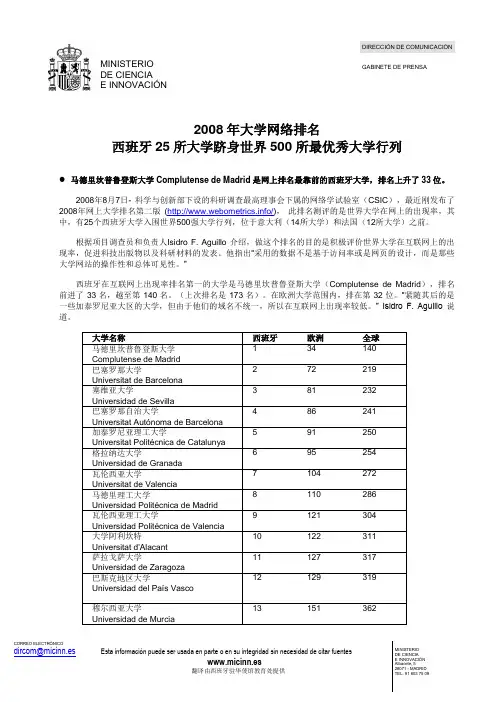
2008年大学网络排名西班牙25所大学跻身世界500所最优秀大学行列马德里坎普鲁登斯大学Complutense de Madrid 是网上排名最靠前的西班牙大学,排名上升了33位。
2008年8月7日- 科学与创新部下设的科研调查最高理事会下属的网络学试验室(CSIC ),最近刚发布了2008年网上大学排名第二版 (/), 此排名测评的是世界大学在网上的出现率,其中,有25个西班牙大学入围世界500强大学行列,位于意大利(14所大学)和法国(12所大学)之前。
根据项目调查员和负责人Isidro F. Aguillo 介绍,做这个排名的目的是积极评价世界大学在互联网上的出现率,促进科技出版物以及科研材料的发表。
他指出“采用的数据不是基于访问率或是网页的设计,而是那些大学网站的操作性和总体可见性。
”西班牙在互联网上出现率排名第一的大学是马德里坎普鲁登斯大学(Complutense de Madrid ),排名前进了33名,越至第140名。
(上次排名是173名)。
在欧洲大学范围内,排在第32位。
“紧随其后的是一些加泰罗尼亚大区的大学,但由于他们的域名不统一,所以在互联网上出现率较低。
” Isidro F. Aguillo 说道。
MINISTERIO DE CIENCIA E INNOVACIÓNDIRECCIÓN DE COMUNICACIÓNGABINETE DE PRENSA互联网上排名最靠前的大学的排名和去年比较几乎没有改变。
排名第一的大学是麻省理工大学(MIT),随后紧跟着的是哈佛大学和斯坦福大学。
其他一些重要的大学比如贝凯利Berkeley, 康奈尔Cornell 或者是多伦托Toronto,也出现在前几名中。
然而,加州理工学院(Caltech)或是约翰霍普金斯大学(Johns Hopkins)由于不恰当的网络策略,排名有些靠后。
在欧洲大学中,德国大学由于其数量众多而地位显著。

北欧留学北欧各国名校推荐汇总瑞典:好大学有以下几所(按照我心中和我接触的瑞典人告诉我的排序,非官方)1 卡罗林斯卡学院(ki)“卡罗林斯卡学院在全世界的高等教育中,是最大的一所单一医学院。
”(wikipedia)其中适合我们申请的只有2个项目master‘s degree programme in biomedicinedegree programme in public health特别是第一个项目,我个人认为无论从学校的名气还是项目本身来看,对于学习生物医学的人都是一个最好的选择2 乌普萨拉大学(uu)北欧最古老的大学,成立于1477年主要介绍3个比较火的项目master programme in computer science 基本是计算机专业的人申请北欧大学的第一选master programme in applied biotechnology 生物技术申请的人似乎也很多master programme in chemistry 和su的化学专业一起应该是北欧最好的imp项目另外,硕士的项目还包括有数学,物理,生物,地球科学等理学科,和法律、英语等专可以说uu是非工科类学生在北欧的首选。
3 斯德哥尔摩大学(su)好学校,好地方,瑞典人心中的top,基本上imp课程也包括所以的非工科专业,与uu不同的是,su的经济学名气很大,可以作为经济学学生的一个选择。
4 隆德大学 (lund)“建于1666年,是现今瑞典境内第二古老的大学。
” (wikipedia)与以上三个学校相比,lun在申请过程中实际上受到更多的关注,主要还是因为除了这所学校综合实力比较强之外,她还拥有一个独立的工学院(lth),其中提供几个特别适合我们电信专业的学生申请的项目。
system-on-chip (soc)北欧口碑最好的soc项目,偏重在模拟电路的设计,这个项目学到的东西实用性很强,多少年来一直都被申请北欧的前辈们所推崇。

【导语】由于⽓候寒冷,农业⽐重较⼩。
⼯业发达⽽且种类繁多,瑞典拥有⾃⼰的航空业、核⼯业、汽车制造业、先进的军事⼯业,以及全球的电讯业和医药研究能⼒。
下⾯是分享的店铺瑞典⼋⼤推荐。
欢迎阅读参考!店铺瑞典⼋⼤推荐 ⼀、卡罗林斯卡学院 位于瑞典斯德哥尔摩的卡罗林斯卡学院是世界的医科⼤学之⼀。
它的愿景是通过研究和教学为改善⼈类健康作出贡献。
该机构⼤约有6 000名学⽣,位于卡罗林斯卡⼤学医院附近。
卡罗林斯卡学院的研究横跨整个医学领域,从基础实验研究到以病⼈为中⼼的研究和护理研究。
该机构是瑞典的学术医学研究机构。
1810年,国王卡尔⼗三世创建了卡罗林斯卡学院,该学院当时是作为⼀所训练外科医⽣的学院。
1861年,学校被授予授予学位的权利,获得了与⼤学同等的地位。
1895年,阿尔弗雷德·诺贝尔(Alfred Nobel)的遗嘱将选择诺贝尔⽣理学或医学奖得主的权利留给了卡罗林斯卡学院(Karolinska Institute)。
从那以后,5名卡罗林斯卡学院的研究⼈员获得了这⼀领域的诺贝尔奖。
⼀九九七年,⾹港理⼯⼤学获颁授⼤学学位。
该机构有两个校区:KI Campus Solna和KI Campus Huddinge,分别位于斯德哥尔摩的西北部和南部。
从市中⼼步⾏或乘⽕车都需要10-15分钟。
除了学⼠和硕⼠学位,卡罗林斯卡学院还提供博⼠学位。
要获得博⼠学位,学⽣必须具备先进的医学和科学⽅法的⼀般知识,以及他们选择在论⽂中探索的研究领域的尖端科学技能。
⼆、隆德⼤学 隆德⼤学成⽴于1666年,是瑞典的⼀所公⽴研究型⼤学,⼀直处于世界顶尖⼤学之列。
该⼤学位于瑞典南部的隆德市(靠近丹麦和德国),在马尔默和赫尔⾟堡也有校区。
它拥有超过4.1万名学⽣(其中3000名是研究⽣)和7000多名员⼯,被认为是北欧的教育和研究机构之⼀。
它还以拥有斯堪的纳维亚最⼴泛的教育项⽬之⼀⽽⾃豪,拥有超过300个学位项⽬和2000个课程。

瑞士留学:萝实学院主要信息介绍导读:本文瑞士留学:萝实学院主要信息介绍,仅供参考,如果能帮助到您,欢迎点评和分享。
萝实学院是一所享有盛名的寄宿学校,始建于1880年,是瑞士最古老的私立学校。
同时,它还是瑞士最大的寄宿学校,现有来自50个国家的340名寄宿生,其中60%来自欧洲,没有任何一个国家的学生比例超过10%。
本学院是瑞士,或许是全球唯一一所拥有两所校园的学校:一所位于Rolle,开设春夏季学期的课程;另外一所地处Gstaad,师生在这里进行冬季学期的学习。
占地35公顷的校园配备有最现代化的学习、体育、艺术和寄宿设施。
主要信息●建校时间:1880年●学生人数:400名住校生●年龄范围:9至18岁的男女学生●校园:两个校区(80 英亩) :春秋季在Rolle(日内瓦湖) ,冬天在Gstaad(格施塔德)●资格认证:新英格兰院校协会(NEASC) ,国际文凭组织(IBO) ,国际学校委员会(CIS) ,法国文凭组织●学生国籍:60 个国家;每个国家所占比例至多为10%学术水平●语言:自由选择法语和英语课程●准备课程:SAT, TOEFL, IGCSE●学位证书:国际文凭(IB)和法国文凭●师生比例:1:4(超过110 名老师的专业团队)●外语:提供各种等级的20多种语言课外活动●30多种运动和艺术项目的日常紧凑训练●文化活动课程,周末探险,卓越挑战,荣誉郊游,演讲者课程和各种各样的社团●坚定地致力于人道主义项目●学校生活:拥有6000校友的强大网络夏令营●在Rolle和Gstaad校区的4次夏令营●9至16岁学生●语言、探险、大量的运动、艺术和远足的多重选择;品味Le Rosey奇趣的特殊项目及设施。
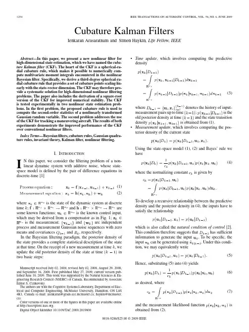
1254IEEE TRANSACTIONS ON AUTOMATIC CONTROL, VOL. 54, NO. 6, JUNE 2009Cubature Kalman FiltersIenkaran Arasaratnam and Simon Haykin, Life Fellow, IEEEAbstract—In this paper, we present a new nonlinear filter for high-dimensional state estimation, which we have named the cubature Kalman filter (CKF). The heart of the CKF is a spherical-radial cubature rule, which makes it possible to numerically compute multivariate moment integrals encountered in the nonlinear Bayesian filter. Specifically, we derive a third-degree spherical-radial cubature rule that provides a set of cubature points scaling linearly with the state-vector dimension. The CKF may therefore provide a systematic solution for high-dimensional nonlinear filtering problems. The paper also includes the derivation of a square-root version of the CKF for improved numerical stability. The CKF is tested experimentally in two nonlinear state estimation problems. In the first problem, the proposed cubature rule is used to compute the second-order statistics of a nonlinearly transformed Gaussian random variable. The second problem addresses the use of the CKF for tracking a maneuvering aircraft. The results of both experiments demonstrate the improved performance of the CKF over conventional nonlinear filters. Index Terms—Bayesian filters, cubature rules, Gaussian quadrature rules, invariant theory, Kalman filter, nonlinear filtering.• Time update, which involves computing the predictive density(3)where denotes the history of input; is the measurement pairs up to time and the state transition old posterior density at time is obtained from (1). density • Measurement update, which involves computing the posterior density of the current stateI. INTRODUCTIONUsing the state-space model (1), (2) and Bayes’ rule we have (4) where the normalizing constant is given byIN this paper, we consider the filtering problem of a nonlinear dynamic system with additive noise, whose statespace model is defined by the pair of difference equations in discrete-time [1] (1) (2)is the state of the dynamic system at discrete where and are time ; is the known control input, some known functions; which may be derived from a compensator as in Fig. 1; is the measurement; and are independent process and measurement Gaussian noise sequences with zero and , respectively. means and covariances In the Bayesian filtering paradigm, the posterior density of the state provides a complete statistical description of the state at that time. On the receipt of a new measurement at time , we in update the old posterior density of the state at time two basic steps:Manuscript received July 02, 2008; revised July 02, 2008, August 29, 2008, and September 16, 2008. First published May 27, 2009; current version published June 10, 2009. This work was supported by the Natural Sciences & Engineering Research Council (NSERC) of Canada. Recommended by Associate Editor S. Celikovsky. The authors are with the Cognitive Systems Laboratory, Department of Electrical and Computer Engineering, McMaster University, Hamilton, ON L8S 4K1, Canada (e-mail: aienkaran@grads.ece.mcmaster.ca; haykin@mcmaster. ca). Color versions of one or more of the figures in this paper are available online at . Digital Object Identifier 10.1109/TAC.2009.2019800To develop a recursive relationship between the predictive density and the posterior density in (4), the inputs have to satisfy the relationshipwhich is also called the natural condition of control [2]. has sufficient This condition therefore suggests that information to generate the input . To be specific, the can be generated using . Under this condiinput tion, we may equivalently write (5) Hence, substituting (5) into (4) yields (6) as desired, where (7) and the measurement likelihood function obtained from (2). is0018-9286/$25.00 © 2009 IEEEARASARATNAM AND HAYKIN: CUBATURE KALMAN FILTERS1255Fig. 1. Signal-flow diagram of a dynamic state-space model driven by the feedback control input. The observer may employ a Bayesian filter. The label denotes the unit delay.The Bayesian filter solution given by (3), (6), and (7) provides a unified recursive approach for nonlinear filtering problems, at least conceptually. From a practical perspective, however, we find that the multi-dimensional integrals involved in (3) and (7) are typically intractable. Notable exceptions arise in the following restricted cases: 1) A linear-Gaussian dynamic system, the optimal solution for which is given by the celebrated Kalman filter [3]. 2) A discrete-valued state-space with a fixed number of states, the optimal solution for which is given by the grid filter (Hidden-Markov model filter) [4]. 3) A “Benes type” of nonlinearity, the optimal solution for which is also tractable [5]. In general, when we are confronted with a nonlinear filtering problem, we have to abandon the idea of seeking an optimal or analytical solution and be content with a suboptimal solution to the Bayesian filter [6]. In computational terms, suboptimal solutions to the posterior density can be obtained using one of two approximate approaches: 1) Local approach. Here, we derive nonlinear filters by fixing the posterior density to take a priori form. For example, we may assume it to be Gaussian; the nonlinear filters, namely, the extended Kalman filter (EKF) [7], the central-difference Kalman filter (CDKF) [8], [9], the unscented Kalman filter (UKF) [10], and the quadrature Kalman filter (QKF) [11], [12], fall under this first category. The emphasis on locality makes the design of the filter simple and fast to execute. 2) Global approach. Here, we do not make any explicit assumption about the posterior density form. For example, the point-mass filter using adaptive grids [13], the Gaussian mixture filter [14], and particle filters using Monte Carlo integrations with the importance sampling [15], [16] fall under this second category. Typically, the global methods suffer from enormous computational demands. Unfortunately, the presently known nonlinear filters mentioned above suffer from the curse of dimensionality [17] or divergence or both. The effect of curse of dimensionality may often become detrimental in high-dimensional state-space models with state-vectors of size 20 or more. The divergence may occur for several reasons including i) inaccurate or incomplete model of the underlying physical system, ii) informationloss in capturing the true evolving posterior density completely, e.g., a nonlinear filter designed under the Gaussian assumption may fail to capture the key features of a multi-modal posterior density, iii) high degree of nonlinearities in the equations that describe the state-space model, and iv) numerical errors. Indeed, each of the above-mentioned filters has its own domain of applicability and it is doubtful that a single filter exists that would be considered effective for a complete range of applications. For example, the EKF, which has been the method of choice for nonlinear filtering problems in many practical applications for the last four decades, works well only in a ‘mild’ nonlinear environment owing to the first-order Taylor series approximation for nonlinear functions. The motivation for this paper has been to derive a more accurate nonlinear filter that could be applied to solve a wide range (from low to high dimensions) of nonlinear filtering problems. Here, we take the local approach to build a new filter, which we have named the cubature Kalman filter (CKF). It is known that the Bayesian filter is rendered tractable when all conditional densities are assumed to be Gaussian. In this case, the Bayesian filter solution reduces to computing multi-dimensional integrals, whose integrands are all of the form nonlinear function Gaussian. The CKF exploits the properties of highly efficient numerical integration methods known as cubature rules for those multi-dimensional integrals [18]. With the cubature rules at our disposal, we may describe the underlying philosophy behind the derivation of the new filter as nonlinear filtering through linear estimation theory, hence the name “cubature Kalman filter.” The CKF is numerically accurate and easily extendable to high-dimensional problems. The rest of the paper is organized as follows: Section II derives the Bayesian filter theory in the Gaussian domain. Section III describes numerical methods available for moment integrals encountered in the Bayesian filter. The cubature Kalman filter, using a third-degree spherical-radial cubature rule, is derived in Section IV. Our argument for choosing a third-degree rule is articulated in Section V. We go on to derive a square-root version of the CKF for improved numerical stability in Section VI. The existing sigma-point approach is compared with the cubature method in Section VII. We apply the CKF in two nonlinear state estimation problems in Section VIII. Section IX concludes the paper with a possible extension of the CKF algorithm for a more general setting.1256IEEE TRANSACTIONS ON AUTOMATIC CONTROL, VOL. 54, NO. 6, JUNE 2009II. BAYESIAN FILTER THEORY IN THE GAUSSIAN DOMAIN The key approximation taken to develop the Bayesian filter theory under the Gaussian domain is that the predictive density and the filter likelihood density are both Gaussian, which eventually leads to a Gaussian posterior den. The Gaussian is the most convenient and widely sity used density function for the following reasons: • It has many distinctive mathematical properties. — The Gaussian family is closed under linear transformation and conditioning. — Uncorrelated jointly Gaussian random variables are independent. • It approximates many physical random phenomena by virtue of the central limit theorem of probability theory (see Sections 5.7 and 6.7 in [19] for more details). Under the Gaussian approximation, the functional recursion of the Bayesian filter reduces to an algebraic recursion operating only on means and covariances of various conditional densities encountered in the time and the measurement updates. A. Time Update In the time update, the Bayesian filter computes the mean and the associated covariance of the Gaussian predictive density as follows: (8) where is the statistical expectation operator. Substituting (1) into (8) yieldsTABLE I KALMAN FILTERING FRAMEWORKB. Measurement Update It is well known that the errors in the predicted measurements are zero-mean white sequences [2], [20]. Under the assumption that these errors can be well approximated by the Gaussian, we write the filter likelihood density (12) where the predicted measurement (13) and the associated covariance(14) Hence, we write the conditional Gaussian density of the joint state and the measurement(15) (9) where the cross-covariance is assumed to be zero-mean and uncorrelated Because with the past measurements, we get (16) On the receipt of a new measurement , the Bayesian filter from (15) yielding computes the posterior density (17) (10) where is the conventional symbol for a Gaussian density. Similarly, we obtain the error covariance where (18) (19) (20) If and are linear functions of the state, the Bayesian filter under the Gaussian assumption reduces to the Kalman filter. Table I shows how quantities derived above are called in the Kalman filtering framework. The signal-flow diagram in Fig. 2 summarizes the steps involved in the recursion cycle of the Bayesian filter. The heart of the Bayesian filter is therefore how to compute Gaussian(11)ARASARATNAM AND HAYKIN: CUBATURE KALMAN FILTERS1257Fig. 2. Signal-flow diagram of the recursive Bayesian filter under the Gaussian assumption, where “G-” stands for “Gaussian-.”weighted integrals whose integrands are all of the form nonGaussian density that are present in (10), linear function (11), (13), (14) and (16). The next section describes numerical integration methods to compute multi-dimensional weighted integrals. III. REVIEW ON NUMERICAL METHODS FOR MOMENT INTEGRALS Consider a multi-dimensional weighted integral of the form (21) is some arbitrary function, is the region of where for all integration, and the known weighting function . In a Gaussian-weighted integral, for example, is a Gaussian density and satisfies the nonnegativity condition in the entire region. If the solution to the above integral (21) is difficult to obtain, we may seek numerical integration methods to compute it. The basic task of numerically computing the integral (21) is to find a set of points and weights that approximates by a weighted sum of function evaluations the integral (22) The methods used to find can be divided into product rules and non-product rules, as described next. A. Product Rules ), we For the simplest one-dimensional case (that is, may apply the quadrature rule to compute the integral (21) numerically [21], [22]. In the context of the Bayesian filter, we mention the Gauss-Hermite quadrature rule; when the is in the form of a Gaussian density weighting functionis well approximated by a polynomial and the integrand in , the Gauss-Hermite quadrature rule is used to compute the Gaussian-weighted integral efficiently [12]. The quadrature rule may be extended to compute multidimensional integrals by successively applying it in a tensorproduct of one-dimensional integrals. Consider an -point per dimension quadrature rule that is exact for polynomials of points for functional degree up to . We set up a grid of evaluations and numerically compute an -dimensional integral while retaining the accuracy for polynomials of degree up to only. Hence, the computational complexity of the product quadrature rule increases exponentially with , and therefore , suffers from the curse of dimensionality. Typically for the product Gauss-Hermite quadrature rule is not a reasonable choice to approximate a recursive optimal Bayesian filter. B. Non-Product Rules To mitigate the curse of dimensionality issue in the product rules, we may seek non-product rules for integrals of arbitrary dimensions by choosing points directly from the domain of integration [18], [23]. Some of the well-known non-product rules include randomized Monte Carlo methods [4], quasi-Monte Carlo methods [24], [25], lattice rules [26] and sparse grids [27]–[29]. The randomized Monte Carlo methods evaluate the integration using a set of equally-weighted sample points drawn randomly, whereas in quasi-Monte Carlo methods and lattice rules the points are generated from a unit hyper-cube region using deterministically defined mechanisms. On the other hand, the sparse grids based on Smolyak formula in principle, combine a quadrature (univariate) routine for high-dimensional integrals more sophisticatedly; they detect important dimensions automatically and place more grid points there. Although the non-product methods mentioned here are powerful numerical integration tools to compute a given integral with a prescribed accuracy, they do suffer from the curse of dimensionality to certain extent [30].1258IEEE TRANSACTIONS ON AUTOMATIC CONTROL, VOL. 54, NO. 6, JUNE 2009C. Proposed Method In the recursive Bayesian estimation paradigm, we are interested in non-product rules that i) yield reasonable accuracy, ii) require small number of function evaluations, and iii) are easily extendable to arbitrarily high dimensions. In this paper we derive an efficient non-product cubature rule for Gaussianweighted integrals. Specifically, we obtain a third-degree fullysymmetric cubature rule, whose complexity in terms of function evaluations increases linearly with the dimension . Typically, a set of cubature points and weights are chosen so that the cubature rule is exact for a set of monomials of degree or less, as shown by (23)Gaussian density. Specifically, we consider an integral of the form (24)defined in the Cartesian coordinate system. To compute the above integral numerically we take the following two steps: i) We transform it into a more familiar spherical-radial integration form ii) subsequently, we propose a third-degree spherical-radial rule. A. Transformation In the spherical-radial transformation, the key step is a change of variable from the Cartesian vector to a radius and with , so direction vector as follows: Let for . Then the integral (24) can be that rewritten in a spherical-radial coordinate system as (25) is the surface of the sphere defined by and is the spherical surface measure or the area element on . We may thus write the radial integral (26) is defined by the spherical integral with the unit where weighting function (27) The spherical and the radial integrals are numerically computed by the spherical cubature rule (Section IV-B below) and the Gaussian quadrature rule (Section IV-C below), respectively. Before proceeding further, we introduce a number of notations and definitions when constructing such rules as follows: • A cubature rule is said to be fully symmetric if the following two conditions hold: implies , where is any point obtainable 1) from by permutations and/or sign changes of the coordinates of . on the region . That is, all points in 2) the fully symmetric set yield the same weight value. For example, in the one-dimensional space, a point in the fully symmetric set implies that and . • In a fully symmetric region, we call a point as a generator , where if , . The new should not be confused with the control input . zero coordinates and use • For brevity, we suppress to represent a complete fully the notation symmetric set of points that can be obtained by permutating and changing the sign of the generator in all possible ways. Of course, the complete set entails where; are non-negative integers and . Here, an important quality criterion of a cubature rule is its degree; the higher the degree of the cubature rule is, the more accurate solution it yields. To find the unknowns of the cubature rule of degree , we solve a set of moment equations. However, solving the system of moment equations may be more tedious with increasing polynomial degree and/or dimension of the integration domain. For example, an -point cubature rule entails unknown parameters from its points and weights. In general, we may form a system of equations with respect to unknowns from distinct monomials of degree up to . For the nonlinear system to have at least one solution (in this case, the system is said to be consistent), we use at least as many unknowns as equations [31]. That is, we choose to be . Suppose we obtain a cu. In this case, we solve bature rule of degree three for nonlinear moment equations; the re) sulting rule may consist of more than 85 ( weighted cubature points. To reduce the size of the system of algebraically independent equations or equivalently the number of cubature points markedly, Sobolev proposed the invariant theory in 1962 [32] (see also [31] and the references therein for a recent account of the invariant theory). The invariant theory, in principle, discusses how to restrict the structure of a cubature rule by exploiting symmetries of the region of integration and the weighting function. For example, integration regions such as the unit hypercube, the unit hypersphere, and the unit simplex exhibit symmetry. Hence, it is reasonable to look for cubature rules sharing the same symmetry. For the case considered above and ), using the invariant theory, we may con( cubature points struct a cubature rule consisting of by solving only a pair of moment equations (see Section IV). Note that the points and weights of the cubature rule are in. Hence, they can be computed dependent of the integrand off-line and stored in advance to speed up the filter execution. where IV. CUBATURE KALMAN FILTER As described in Section II, nonlinear filtering in the Gaussian domain reduces to a problem of how to compute integrals, whose integrands are all of the form nonlinear functionARASARATNAM AND HAYKIN: CUBATURE KALMAN FILTERS1259points when are all distinct. For example, represents the following set of points:Here, the generator is • We use . set B. Spherical Cubature Rule. to denote the -th point from theWe first postulate a third-degree spherical cubature rule that takes the simplest structure due to the invariant theory (28) The point set due to is invariant under permutations and sign changes. For the above choice of the rule (28), the monomials with being an odd integer, are integrated exactly. In order that this rule is exact for all monomials of degree up to three, it remains to require that the rule is exact , 2. Equivalently, to for all monomials for which find the unknown parameters and , it suffices to consider , and due to the fully symmonomials metric cubature rule (29) (30) where the surface area of the unit sphere with . Solving (29) and (30) , and . Hence, the cubature points are yields located at the intersection of the unit sphere and its axes. C. Radial Rule We next propose a Gaussian quadrature for the radial integration. The Gaussian quadrature is known to be the most efficient numerical method to compute a one-dimensional integration [21], [22]. An -point Gaussian quadrature is exact and constructed as up to polynomials of degree follows: (31) where is a known weighting function and non-negative on ; the points and the associated weights the interval are unknowns to be determined uniquely. In our case, a comparison of (26) and (31) yields the weighting function and and , respecthe interval to be tively. To transform this integral into an integral for which the solution is familiar, we make another change of variable via yielding. The integral on the right-hand side of where (32) is now in the form of the well-known generalized GaussLaguerre formula. The points and weights for the generalized Gauss-Laguerre quadrature are readily obtained as discussed elsewhere [21]. A first-degree Gauss-Laguerre rule is exact for . Equivalently, the rule is exact for ; it . is not exact for odd degree polynomials such as Fortunately, when the radial-rule is combined with the spherical rule to compute the integral (24), the (combined) spherical-radial rule vanishes for all odd-degree polynomials; the reason is that the spherical rule vanishes by symmetry for any odd-degree polynomial (see (25)). Hence, the spherical-radial rule for (24) is exact for all odd degrees. Following this argument, for a spherical-radial rule to be exact for all third-degree polyno, it suffices to consider the first-degree genermials in alized Gauss-Laguerre rule entailing a single point and weight. We may thus write (33) where the point is chosen to be the square-root of the root of the first-order generalized Laguerre polynomial, which is orthogonal with respect to the modified weighting function ; subsequently, we find by solving the zeroth-order moment equation appropriately. In this case, we , and . A detailed account have of computing the points and weights of a Gaussian quadrature with the classical and nonclassical weighting function is presented in [33]. D. Spherical-Radial Rule In this subsection, we describe two useful results that are used to i) combine the spherical and radial rule obtained separately, and ii) extend the spherical-radial rule for a Gaussian weighted integral. The respective results are presented as two propositions: Proposition 4.1: Let the radial integral be computed numer-point Gaussian quadrature rule ically by theLet the spherical integral be computed numerically by the -point spherical ruleThen, an by-point spherical-radial cubature rule is given(34) Proof: Because cubature rules are devised to be exact for a subspace of monomials of some degree, we consider an integrand of the form(32)1260IEEE TRANSACTIONS ON AUTOMATIC CONTROL, VOL. 54, NO. 6, JUNE 2009where are some positive integers. Hence, we write the integral of interestwhereFor the moment, we assume the above integrand to be a mono. Making the mial of degree exactly; that is, change of variable as described in Section IV-A, we getWe use the cubature-point set to numerically compute integrals (10), (11), and (13)–(16) and obtain the CKF algorithm, details of which are presented in Appendix A. Note that the above cubature-point set is now defined in the Cartesian coordinate system. V. IS THERE A NEED FOR HIGHER-DEGREE CUBATURE RULES? In this section, we emphasize the importance of third-degree cubature rules over higher-degree rules (degree more than three), when they are embedded into the cubature Kalman filtering framework for the following reasons: • Sufficient approximation. The CKF recursively propagates the first two-order moments, namely, the mean and covariance of the state variable. A third-degree cubature rule is also constructed using up to the second-order moment. Moreover, a natural assumption for a nonlinearly transformed variable to be closed in the Gaussian domain is that the nonlinear function involved is reasonably smooth. In this case, it may be reasonable to assume that the given nonlinear function can be well-approximated by a quadratic function near the prior mean. Because the third-degree rule is exact up to third-degree polynomials, it computes the posterior mean accurately in this case. However, it computes the error covariance approximately; for the covariance estimate to be more accurate, a cubature rule is required to be exact at least up to a fourth degree polynomial. Nevertheless, a higher-degree rule will translate to higher accuracy only if the integrand is well-behaved in the sense of being approximated by a higher-degree polynomial, and the weighting function is known to be a Gaussian density exactly. In practice, these two requirements are hardly met. However, considering in the cubature Kalman filtering framework, our experience with higher-degree rules has indicated that they yield no improvement or make the performance worse. • Efficient and robust computation. The theoretical lower bound for the number of cubature points of a third-degree centrally symmetric cubature rule is given by twice the dimension of an integration region [34]. Hence, the proposed spherical-radial cubature rule is considered to be the most efficient third-degree cubature rule. Because the number of points or function evaluations in the proposed cubature rules scales linearly with the dimension, it may be considered as a practical step for easing the curse of dimensionality. According to [35] and Section 1.5 in [18], a ‘good’ cubature rule has the following two properties: (i) all the cubature points lie inside the region of integration, and (ii) all the cubature weights are positive. The proposed rule equal, positive weights for an -dimensional entails unbounded region and hence belongs to a good cubature family. Of course, we hardly find higher-degree cubature rules belonging to a good cubature family especially for high-dimensional integrations.Decomposing the above integration into the radial and spherical integrals yieldsApplying the numerical rules appropriately, we haveas desired. As we may extend the above results for monomials of degree less than , the proposition holds for any arbitrary integrand that can be written as a linear combination of monomials of degree up to (see also [18, Section 2.8]). Proposition 4.2: Let the weighting functions and be and . such that , we Then for every square matrix have (35) Proof: Consider the left-hand side of (35). Because a positive definite matrix, we factorize to be , we get Making a change of variable via is .which proves the proposition. For the third-degree spherical-radial rule, and . Hence, it entails a total of cubature points. Using the above propositions, we extend this third-degree spherical-radial rule to compute a standard Gaussian weighted integral as follows:ARASARATNAM AND HAYKIN: CUBATURE KALMAN FILTERS1261In the final analysis, the use of higher-degree cubature rules in the design of the CKF may marginally improve its performance at the expense of a reduced numerical stability and an increased computational cost. VI. SQUARE-ROOT CUBATURE KALMAN FILTER This section addresses i) the rationale for why we need a square-root extension of the standard CKF and ii) how the square-root solution can be developed systematically. The two basic properties of an error covariance matrix are i) symmetry and ii) positive definiteness. It is important that we preserve these two properties in each update cycle. The reason is that the use of a forced symmetry on the solution of the matrix Ricatti equation improves the numerical stability of the Kalman filter [36], whereas the underlying meaning of the covariance is embedded in the positive definiteness. In practice, due to errors introduced by arithmetic operations performed on finite word-length digital computers, these two properties are often lost. Specifically, the loss of the positive definiteness may probably be more hazardous as it stops the CKF to run continuously. In each update cycle of the CKF, we mention the following numerically sensitive operations that may catalyze to destroy the properties of the covariance: • Matrix square-rooting [see (38) and (43)]. • Matrix inversion [see (49)]. • Matrix squared-form amplifying roundoff errors [see (42), (47) and (48)]. • Substraction of the two positive definite matrices present in the covariant update [see (51)]. Moreover, some nonlinear filtering problems may be numerically ill-conditioned. For example, the covariance is likely to turn out to be non-positive definite when i) very accurate measurements are processed, or ii) a linear combination of state vector components is known with greater accuracy while other combinations are essentially unobservable [37]. As a systematic solution to mitigate ill effects that may eventually lead to an unstable or even divergent behavior, the logical procedure is to go for a square-root version of the CKF, hereafter called square-root cubature Kalman filter (SCKF). The SCKF essentially propagates square-root factors of the predictive and posterior error covariances. Hence, we avoid matrix square-rooting operations. In addition, the SCKF offers the following benefits [38]: • Preservation of symmetry and positive (semi)definiteness of the covariance. Improved numerical accuracy owing to the fact that , where the symbol denotes the condition number. • Doubled-order precision. To develop the SCKF, we use (i) the least-squares method for the Kalman gain and (ii) matrix triangular factorizations or triangularizations (e.g., the QR decomposition) for covariance updates. The least-squares method avoids to compute a matrix inversion explicitly, whereas the triangularization essentially computes a triangular square-root factor of the covariance without square-rooting a squared-matrix form of the covariance. Appendix B presents the SCKF algorithm, where all of the steps can be deduced directly from the CKF except for the update of the posterior error covariance; hence we derive it in a squared-equivalent form of the covariance in the appendix.The computational complexity of the SCKF in terms of flops, grows as the cube of the state dimension, hence it is comparable to that of the CKF or the EKF. We may reduce the complexity significantly by (i) manipulating sparsity of the square-root covariance carefully and (ii) coding triangularization algorithms for distributed processor-memory architectures. VII. A COMPARISON OF UKF WITH CKF Similarly to the CKF, the unscented Kalman filter (UKF) is another approximate Bayesian filter built in the Gaussian domain, but uses a completely different set of deterministic weighted points [10], [39]. To elaborate the approach taken in the UKF, consider an -dimensional random variable having with mean and covariance a symmetric prior density , within which the Gaussian is a special case. Then a set of sample points and weights, are chosen to satisfy the following moment-matching conditions:Among many candidate sets, one symmetrically distributed sample point set, hereafter called the sigma-point set, is picked up as follows:where and the -th column of a matrix is denoted ; the parameter is used to scale the spread of sigma points by from the prior mean , hence the name “scaling parameter”. Due to its symmetry, the sigma-point set matches the skewness. Moreover, to capture the kurtosis of the prior density closely, it is sug(Appendix I of [10], gested that we choose to be [39]). This choice preserves moments up to the fifth order exactly in the simple one-dimensional Gaussian case. In summary, the sigma-point set is chosen to capture a number as correctly as of low-order moments of the prior density possible. Then the unscented transformation is introduced as a method that are related to of computing posterior statistics of by a nonlinear transformation . It approximates the mean and the covariance of by a weighted sum of projected space, as shown by sigma points in the(36)(37)。


University of Boras
布罗斯大学
项目优势:
1.靠近瑞典第2大城市哥德堡,交通方便
2.布罗斯是瑞典的物流中心和纺织中心
3.学校以就业为导向,工程,纺织瑞典前列
学校概况
布罗斯大学学院成立于1977年, 学校师生人数大约11,500人。
学校距离瑞典第二大城市哥德堡距离很近。
学校由6个院校组成:图书情报学院,商业和信息学院,工程学院,教育和行为学院,纺织学院,卫生学院。
学校的很多英语授课专业在瑞典是唯一的, 比如服装和纺织学院提供英语授课的硕士。
学校和公司保持很好关系, 很多学校项目研究是瑞典公司赞助。
2005年学校向瑞典教育部递交申请, 希望成为瑞典第一所职业为导向的大学。
课程介绍
英文授课本科 (三年)
工业工程-商业商务工程
英文授课硕士 (1年)
1. 应用纺织管理
2. 工商管理
3. 时装管理–时装营销及销售
4. 纺织技术
5. 信息学
6. 工业工程–物流管理
英文授课硕士 (2年)
1.时装与纺织设计–时尚设计
2.纺织工程
3.纺织管理–时尚管理
4.纺织管理–纺织价值链管理
5.信息学–企业系统设计与IT
6.资源回收–工业生物技术
7.资源回收–可持续工程
8.时装与纺织品设计–纺织品设计
入学要求:相关专业本科毕业,学士学位;托福550/213/79或者雅思6.0以上
入学时间:八月中旬。
2021年瑞典名校一览表瑞典有哪些好大学
瑞典的大学受到国情地域的影响,数量不算很多,但是知名的院校比例还是比较高的。
下面就由带来2021年瑞典名校一览表瑞典有哪些好大学?
是一所检具历史感和现代化的高等学府,在1666年就已经建立,几百年的发展足够它将学院和专业进行不断地完善,提供的教学和研究都是非常优质的,能够满足学生的需求。
在最新的QS排名中位于第92名,而且排在欧洲的TOP10之内,在学生的满意度调查中位于瑞典首位,专业的综合实力基本上都可以排进国家的前三名,综合素质是很高的。
同样是综合性的院校,学院设置有八个,专业接近60个,可以为留学生提供比较全面的选择,而且在配套的设施和服务上也是比较齐全的,当然申请的难度也不会小,需要认真准备。
在QS的综合排名不算高,在200名左右,但是医科相关学科也拥有很亮眼的表现,可以进入到TOP50的行列,名气和实力是相匹配的,学医的学生首选这所大学。
早在1477年就已经成立,而且还是北欧的第一所高校,是作为奠基者而存在的院校,而且在教学上,更加重视理论的内容一些,对科研的经费投入会更多一些,在成果上也是比较丰富的。
新的QS排在116名的位置,可见其实力的强劲,而且学校虽然建校时间长,但是却并不故步自封,始终坚持更新换代,并且重视新科技,大家在这里学习会有一个很好的开放性氛围。
是瑞典规模最大的学校,目前学生的数量超过了7万名,教职员工你在5000名以上,而师资队伍中,不乏有世界知名的人才和泰斗,在科研方面也有很不错的表现。
不过学校在专业的表现上比较偏科,目前综合排名在190名左右,人文和社会科学,以及法学却能够进入到世界顶尖的位置,资源配置上也会相对要齐全一些。

首先介绍一下瑞典的卡罗林斯卡大学。
卡罗林斯卡大学是北欧最大的医药大学,大学的三分之二是位于瑞典的首都地区。
在座的诸位可能对欧洲不是特别熟悉,所以你们可能感到特别好奇,就是卡罗林斯卡大学座落在哪儿呢?瑞典是一个北欧国家。
瑞典的邻国有挪威、芬兰,南部是丹麦,我们和波兰、比利时接壤。
卡罗林斯卡大学下边有六个分院,总部主要是搞医学的,当然还有社会科学和其他学科的研究领域。
我在这里强调一点,瑞典的医学研究有非常良好和悠久的历史。
北欧这些国家在医药方面都有非常悠久的历史,我们的医药研究成果对整个世界都产生了非常重要的影响。
我们在医学研究方面曾经有诺贝尔生物学奖的获得者,他们在医药方面的研究成果对整个人类作出了贡献。
卡罗林斯卡大学下边有六个分院,总部主要是搞医学的,当然还有社会科学和其他学科的研究领域。
我在这里强调一点,瑞典的医学研究有非常良好和悠久的历史。
北欧这些国家在医药方面都有非常悠久的历史,我们的医药研究成果对整个世界都产生了非常重要的影响。
我们在医学研究方面曾经有诺贝尔生物学奖的获得者,他们在医药方面的研究成果对整个人类作出了贡献。
当然,在国际范围内,我们都有很多合作者。
第二,我们在临床医学方面也有非常好的研究和应用成果。
我们所有的临床医生23%都是获得博士学位的,这个比例在国际上是非常高的,这一点是非常重要的。
也就是说,我们的临床医生大夫和研究者获得博士的比例特别高。
在大学里边,这个比例就更高了,超过25%的大学教授拥有博士学位。
在医药方面,我们的成果也是非常丰硕的。
在瑞典有2家非常大的医药生产厂家,这些医药生产厂家非常重视和大学开展医药方面的研究和合作,两个生产厂家一个在瑞典的北部,一个在瑞典的南部。
瑞典非常大的医药公司和大学合作,这样他们在研发方面才有非常好的成果。
我们对病人进行了大量的研究,对每一个病人都保存了病历档案,在整个病理学的研究方面,覆盖的病人人数也非常多。
下面我讲一下诺贝尔奖。
诺贝尔奖是非常重要的奖项,它是瑞典发起的奖项。
瑞典三大名校介绍隆德大学留学申请难不难
瑞典并不大,所以大学的数量也不算多,但是也是有不少名校的,大家要以名校为目标。
今天就跟着看看瑞典三大名校介绍隆德大学留学申请难不难?
Lund University成立于1666年,不仅是瑞典最古老的院校,也是欧洲建校历史最长的大学之一,经过几百年的发展,既有了实力,又打出了名气,成为了瑞典教育的标杆。
在最新的QS排名中,它的综合实力排在第60位,是真正的世界百强;而在欧洲区域内的排名,在前十名以内,这是非常好的成绩,大家可以不用担心教学。
而且每年瑞典的增幅,还会投入大量的资金支持学校的硬件设施建设,并且还会有项目的专门支持,可以最大程度上提升学校的整体实力,保持领先地位。
始建于1477年的Uppsala University,是瑞典最受欢迎的大学之一,位于美丽的乌普萨拉,享受着个古典文化的艺术的熏陶,能够近距离的接触欧洲传统文化。
在最新的QS排名中,它的综合实力排在第75位,同样也是世界百强;而且在国内的知名度也很高,受到雇主的欢迎,普通民众对于学历的认可度非常高。
学校并不是理所综合大学,它的专业设置,更偏向于文法医门类,培养了众多优秀的艺术家、医生和医学研究者,以及文学家和哲学家。
成立于1827年,在三者中算是比较年轻的,它是一所工学院,是公立的理工类学府,和教学同样出色的,是其研究能力和水平,开展了多项研究项目。
在最新的QS排名中,它的综合实力排在第92位,虽然排名较低,但是其专业专业高,尤其是理工科的专业分支,基本上就能够进入TOP50。
瑞典厄勒布鲁⼤学简介
学校名称:瑞典厄勒布鲁⼤学 Örebro Universitet
所在位置:瑞典,厄勒布鲁市
学费:28000 欧元
录取率:0.864
瑞典厄勒布鲁⼤学 Orebro University成⽴于1977年,现在正在经历快速变⾰时期。
学校和周围的公司,⼯⼚保持良好的合作关系。
在校⽣有13,500名学⽣, 1300名教职⼯, 80多个专业, 12个院系。
位置处在瑞典的中部,交通⽅便。
课程设置
-⼯商管理;计算机科学;经济学;统计学;⼈⼝学;教育学;⼈⽂科学;⾳乐;体育;健康学;饭店管理;⾃然科学;社会科学;科技
图书馆及计算机资源
图书馆收藏瑞典和世界范围的报纸、期刊、杂志、唱⽚、光盘等,适合于⼤学各专业领域的需要。
计算机⽹络管理,可从其他图书馆调集资料和图⽚。
⼤学中⼼⽹络设备设置在计算机⼤楼。
学⽣服务
学校设施齐备,校园内设有图书馆、⽂化中⼼、⾏政管理⼤楼、餐馆、书店、运动场。
学⽣会有⾃⼰的刊物和⼴播站。
学⽣活动也很丰富,有⾳乐会、运动会和演讲活动。
课程设置 (硕⼠)
Economics and econometrics 经济学;
Education for democracy and social justice 民主和社会公平教育
Electronic government电⼦政府; Global Journalism全球传媒
Robotics and intelligent systems 机器⼈和智能系统
⼊学条件:⼤学相关专业毕业,IELTS:6分以上。
瑞典布罗斯大学简介布罗斯大学(瑞典语为H?gskolan i Bor?s)位于瑞典布罗斯,建成于1977年,是瑞典的一所公立大学院。
布罗斯大学是一所拥有6个系的现代化大学院,包括图书馆教育与情报学系,商务和信息学系,时装及纺织学系,行为学和教育科学系及该工程和卫生科学系。
该校处在布罗斯的市中心,现有11800名在校生和600名员工。
布罗斯大学提供工业,生物科技,经济学,信息技术,教育学,工程学,护理学等学位的学习,同时也是瑞典图书管理员的培养基地。
另外,得益于布罗斯市纺织业悠久的历史,布罗斯大学时装及纺织学系因而有着不错的实力,该系位于一座古老的纺织工厂里,因此其学生有着得天独厚的条件实地使用纺织机和制作纺织品。
布罗斯大学还开设了商业法律,设计及管理方面的课程。
布罗斯大学正努力向以专业为中心的研究性大学进军,同时也为成为瑞典第四大警察学院而奋斗。
申请布罗斯大学的理由:1. 学校地点处于瑞典南部,气候较好2. 学校不收取学费3. 硕士课程为英语授课4. 学校为瑞典公立学校5. 教学质量高,录取学生保证安排住宿英语授课3年本科项目 (Business Engineering)学生直接到瑞典攻读英语授课的本科, 无需读任何预科, 本科3年全免费学习. 本科期间学生将可以选择土木工程或者机械工程作为本科的专业, 同时学习商业知识. 毕业后本科学位得到欧洲, 美国等发达国家认可, 同时学位也可以得到中国教育部的认可.第一年将学习理工和商科的一些基础知识第二年学生将学习经济, 物流, 质量管理,项目管理和语言, 以及一些工程类的课程第三年学生将选择土木工程或者机械工程作为自己的专业课程学习.读书期间将有机会交流到其它国家读书 !申请要求:学生需高中毕业或者以上(高三在读也可以),高中阶段学习过数学,化学等高中阶段理工知识(提供公证件), 学生雅斯水平在6分以上(国际班上课, 该专业学生限招50人)学校硕士专业介绍1.应用纺织管理 Applied textile management (一年制硕士)要求:纺织管理或纺织技术方面大四或者本科毕业2.工业工程-质量&环境管理Industrial Engineering- Quality and Environmental Management (一年制硕士)要求:工业、土木、机械、化学、电气、计算机工程或其他相关专业本科毕业。
瑞典厄勒布鲁大学Orebro University学校概况:学校成立于1977年,现在正在经历快速变革时期。
学校和周围的公司,工厂保持良好的合作关系。
在校生有13,500名学生,1300名教职工,80多个专业,12个院系。
学校特色以及概况厄勒布鲁大学,建立于1967年,位于厄勒布鲁市,它处于瑞典的中部。
学校有超过14500名学生及1300多名教职员工,并提供涉及50个领域的80多个学习项目及800多门课程。
学校共设12个学院,硕士课程可供学习的专业有:计量经济学、电子化政府管理、机器人技术和智能系统、全球新闻,其中全球新闻专业是用英语授课的。
厄勒布鲁大学位于距厄勒布鲁市中心1.5英里的Almby,绿树环绕。
1977年瑞典高等教育改革时期建立,前身是乌普萨拉大学社会学院和公共管理学院。
发展很快,目前拥有11,500名学生和850名教职员,每学期接收100名交换留学生。
瑞典厄勒布鲁大学优势专业财经类、法律、纺织与服装、工程技术、管理、环境、建筑、教育、理科学、旅游、农林类、人文艺术、社科类、生物、体育、新闻传播、信息科学、医学、语言、自然科学,体育和运动·入学条件有哪些?本科课程:高中毕业,托福550分或雅思5.5分(单科不低于4.5)硕士课程:相关专业本科毕业,学士学位;托福550或者雅思6.0以上·我什么时候开始申请?4月10月·我要准备多少资金来留学?免学费生活费:每月生活费大约7000SEK,一年合计RMB7-8万元. 提供住宿约3000-5000/月上海财经与瑞典厄勒布鲁大学国际硕士预科项目2011年春季招生计划•项目介绍瑞典厄勒布鲁大学国际硕士预科项目,是上海财经大学和瑞典厄勒布鲁大学合作开发的、面向广大本科毕业生或本科四年级在读学生招生的硕士预科项目。
针对中国学生英语运用能力相对薄弱和国内专业课程设置与国外知名院校确有部分差异的客观情况,合作双方共同设计了一套科学完整的教学内容,旨在通过国内半年的学习,帮助学生全面提高英语水平,进一步夯实经济学和统计学等学科基础知识,为学生顺利完成国外硕士阶段学习打下坚实基础。
高岩任期内工作总结高岩任期内工作总结高岩任期内工作总结(20xx.10-20xx.10)我于20xx年10月份担任管理学院常务副院长,全面主持学院的行政工作,同时分管学科建设、师资队伍建设、财务工作和国际交流。
自主持工作以来,我始终坚持围绕学校中心工作,认真贯彻学校的各项工作部署,以党的理论方针为指导,积极探索学院发展新途径。
在任期间,我一直为把管理学院建成国际知名、国内一流的学院不懈努力着。
3年来,在学校党政班子的正确领导下,在学院总支、行政班子和全院教师的大力支持下,我的各项工作取得了一些成绩。
一、顺利完成学院搬迁工作。
根据学校的发展规划和工作部署,管理学院于20xx年4月份历时2个月整体搬迁至南校区。
我全面负责学院的搬迁工作,并为搬迁工作的顺利开展和有序进行做好组织和协调工作,成立搬迁领导小组,明确责任分工,分批按期组织进行。
20xx年6月份,在全院教职工的理解和配合下,学院搬迁工作圆满完成,教师的教学、科研环境得到较大改善,为教师在校期间的工作和学期提供了良好的环境和硬件支撑。
同时,搬迁期间的教学、科研工作,有序进行,稳步推进。
二、整合学科资源根据学院的发展定位和学科规划,20xx年上半年学院进行了机构调整工作。
新组建了9个系、1专业学位中心,使学科设置更趋合理。
1/4学院的学科建设工作也取得新的进展,成功申报了工商管理、交通运输工程、统计学3个一级硕士点,以及工程管理、国际商务、公共管理3个全日制专业硕士学位点。
6个新学位点的取得,拓展了我院学科发展的新局面。
20xx年5月上海市教委启动了上海高校一流学科申报工作,管理学院认真组织了“管理科学与工程”、“系统科学”2个博士学科申报上海市一流学科,并申报成功。
其中我直接负责的“系统科学”学科在完成材料函审环节后,凭借在全国的一定优势和影响力,跳过答辩评审环节,直接入选上海高校一流学科。
三、引进高素质人才根据管理学院的整体师资情况和我院各学科的师资要求,在师资队伍建设方面,加快高素质人才的引进力度,积极引进高端人才。
360教育集团介绍:布罗斯大学学院成立于1977年。
学校师生人数大约11,500人.学校距离瑞典第二大城市哥德堡距离不远。
学校由6个院校组成:图书情报学院,商业和信息学院,工程学院,教育和行为学院,纺织学院生学院。
学校的很多英语授课专业在瑞典是唯一的,比如服装和纺织学院提供英语授课的硕士。
学校和公司保持很好关系,很多学校项目研究是瑞典公司赞助。
2005年学校向瑞典教育部递交申请,希望成为瑞典第一所职业为导向的大学.
瑞典布罗斯大学硕士专业设置:
1.应用纺织管理 Applied textile management (一年制硕士)
要求:纺织管理或纺织技术方面大四或者本科毕业
2.工业工程-质量&环境管理Industrial Engineering- Quality and Environmental Management (一年制硕士)
要求:工业、土木、机械、化学、电气、计算机工程或其他相关专业本科毕业。
3.物流管理 Logistics Management (一年制硕士)
要求:工业工程或相关专业本科毕业。
4.生物医药工程――biomedical engineering(一年制硕士)
要求:电气工程或其他相关专业本科毕业
5. 纺织技术―――Textile Technology (一年制硕士)
要求:纺织技术本科毕业。
6. 可持续技术-资源恢复―sustainable technology --–resources recovery (两年制硕士)
要求:土木、机械、化学工程或相关专业本科毕业。
7.工业生物技术 Industrial Biotechnology (两年制硕士)
要求:化学工程或相关专业如化学、微生物、药学等本科毕业。
8.时装及纺织品设计 Fashion and Textile Design (两年制硕士)
要求:服装、纺织品设计或其他相关设计专业本科毕业
瑞典布罗斯大学申请信息:
学生需高中毕业或者以上(高三在读也可以),高中阶段学习过数学,
化学等高中阶段理工知识(提供公证件), 学生雅斯水平在6分以上 (国际班上课, 该专业学生限招50人,学校将在12月初左右到中国来面试学生)
申请材料:
1.大学本科毕业证,学位证公证(大四学生提供学校中英文在读证明,需要加盖学校公章)
2.大学成绩公证(平均成绩需75分以上)
3.英语成绩比如雅斯至少5,5分
4.护照第一页复印件(或者身份证复印件)
5.个人简历。