抖动和眼图的视觉分析
- 格式:pdf
- 大小:4.05 MB
- 文档页数:63


抖动和眼图的视觉化分析抖动为实际数据与其理想位置的时间偏差TIE 为信号相对于标准时钟或者标准信号的定时误差TIE 在高速数字系统中即为抖动…0.0ns0.990ns 2.000ns 2.980ns 4.000nsP2P3P4P1TIE0.000ns-0.010ns0.000ns-0.020ns眼图是怎么形成的?Random Jitter(随机抖动)•随机抖动符合高斯型分布•直方图(估计) ↔ pdf(数学模型)•抖动峰峰值=无穷大…无界!1-sigma or RMS 7-sigma•内部热能现象•Flicker Noise, Shot Noise •热能的原子与分子振动•分子的解体•外部的宇宙射线Deterministic Jitter(确定性抖动)•确定性抖动是非高斯分布并且有界Peak-to-PeakPeriodic Jitter(周期性抖动)•TIE 随时间的变化是重复的、周期性的•Periodic jitter 和相位调制(PM)是等效的Peak-to-Peak•系统时钟(抖动频率在MHz 量级)•开关电源(抖动频率在KHz 量级)Duty Cycle distortion(占空比失真)•上升时间和下降时间不对称•或者测试时参考电平选择不当0.0v-0.1vInter-Symbol Interference(码间干扰抖动)•DDJ 或PDJ –数据相关性抖动或码型相关性抖动,和ISI的术语是等价的.•码型是如何影响随后的比特位的?◦由于传输链路的效应、反射等换个角度看抖动,时域看看我们有了什么视角?抖动视觉化–时间趋势图▪直方图告诉了我们分布,但是只有统计特性,缺少了时间信息▪时间趋势图可以直观告诉我们波形里是否有特定频率的调制▪下图为5个周期SSC @ 30khz抖动视觉化Gaussian Random Noise Sinusoidal Jitter抖动视觉化–频谱图▪从频域上观测抖动▪抖动中决定性的频率成分会在谱线上明显超出噪底哪个眼图好?哪个直方图好?视觉化眼图和抖动的问题?浴盆曲线误码率是关键vs. UI 张开程度•For a given position in the time there’s a given probability of error –“BER ”, Bit Error Ratio•For a given position in the time there’s a given probability of signal crossing –PDF , probability density function1 UIP r o b a b i l i t y o f ‘h i t ’P r o b a b i l i t y o f E r r o r –B E R基于示波器分析的浴盆曲线Rj δδ/Dj δδ与Tj @ BERAssume bi-modal distribution (dual-Dirac), measure Tj at two BER Fit curve to points, slope is Rj, Intercept is DjMeasuredTj @ 10-7MeasuredTj @ 10-4½Dj δδ½xRj δδEstimatedTj @ 10-12x≈7.4σx≈10.4σx≈14.1σ双狄拉克模型Conditions: only where Gaussian.抖动类型分析•抖动分离为误码产生的根本原因提供了更精确的定位和分析方法•抖动分析方法,参照T11 MJSQ ,已经被工业界广泛接受Constituent Components of Jitter= Unbounded= Bounded Total Jitter(TJ)Duty-Cycle Jitter (DCD)Data Dependent Jitter (DDJ)Periodic Jitter(PJ)Deterministic Jitter (DJ)Random Jitter(RJ)Jitter Visualization –Bathtub Plot▪Shows the Eye Opening at a Specified BER Level▪Note the eye closure of System I vs. System II due to the RJ-RJ is unbounded so the closure increases as BER level increases▪System I has .053UI of RJ with no PJ▪System II has .018UI of RJ and .14UI of PJ @ 5 and 10MhzSystem I System ISystem II System IITektronix -Innovators of Jitter Analysis •1998First Real-Time Scope Based Jitter Analysis Software•2002 Invented SW Based PLL Clock Recovery and the Spectral Approach for Jitter Separation•2004–Invented RT Eye rendering on a Real Time Scope•2004-First vendor to support both modeled (Dual-Dirac) and measured (Spectral) jitter methods •2005-Invented measurements with Jitter and Noise reconciliation•2011-First scope vendor with BUJ support•2015–RT Noise Analysis and Sampling BER and PDF Mask Testing抖动和眼图的视觉化眼图怎么切割的?时钟决定!TIE 抖动需要参考时钟•参考时钟提取的过程就是时钟恢复•参考时钟有几种确定的方式:◦Constant Clock with Minimum Mean Squared ErrorThis is the mathematically “ideal” clockBut, only applicable when post-processing a finite-length waveformBest for showing very-low-frequency effectsAlso shows very-low-frequency effects of scope’s timebase◦Phase Locked Loop (e.g. Golden PLL)Tracks low-frequency jitter (e.g. clock drift)Models “real world” clock recovery circuits very well◦Explicit ClockThe clock is not recovered, but is directly probed◦Explicit Clock (Subrate)The clock is directly probed, but must be multiplied up by some integral factorImportance of Clock Recovery•From spec, “The jitter measurement device shall comply with the JTF”.•How do I verify JTF?◦JTF is difference between input clock (ref) and input clock(unfiltered)◦Use 1100b or 0011b pattern (proper 50% transition density)◦Check 1) LF attenuation, 2) -3 dB corner frequency, and 3) slope23JTF vs PLL Loop Bandwidth•Configuring the correct PLL settings is key to correctmeasurements•Most standards have a reference/defined CR setup◦For example, USB 3.0 uses a Type II with JTF of 4.9Mhz•Type I PLL◦Type I PLL has 20dB of roll off per decade◦JTF and PLL Loop Bandwidth are Equal•Type 2 PLL◦Type II PLL has 40dB of roll off per decade◦JTF and PLL Loop Bandwidth are not Equal▪For example, USB 3.0 uses a Type 2 PLL with a JTF of 4.9Mhz.The corresponding loop bandwidth is 10.126 Mhz▪Setting the Loop Bandwidth as opposed to JTF will lead to24PLL Loop Bandwidth vs. Jitter Transfer Function(JTF)JTF Filtering Effects based on different PLL bandwidthsf3dB= 30 kHz f3dB= 300 kHz f3dB= 3 MHzJitter for Busy People Hints, Tips and Common ErrorsUsing the Jitter Analysis Tools•Issues manifested in different layers of theprotocol stack◦Crosstalk, jitter, reflections, skew◦Disparity, encoding or CRC errors•Where do I start debugging?•Jitter and Eye Diagram Tools◦Oscilloscope-based for quick results▪Fast jitter measurements with▫‘One Button’ Jitter Wizard▪Compare timing, jitter, eye, amplitude measurements▪User-definable clock recovery, filters, pass/fail limits, andreference levelsMore Hints for Successful Jitter Analysis•Clock Recovery has a great deal of influence on jitter results. Think about what you’re trying to accomplish.◦Constant-Clock is the most “unbiased”Often best if you’re trying to see very-low-frequency effectsBut it can also show wander in the scope’s timebase◦PLL recovery can model what a real data receiver will seeIt can track and remove low-frequency effects, allowing you to “see through” to the jitter that really contributes to eye closur e ◦Explicit-Clock is appropriate if your design uses a forwarded clockMake sure your probes are deskewedHints for looking at Spread-Spectrum Clock•If you don’t want to see the SSC effects, use TIE and PLL clock recovery with a bandwidth of at least 1 MHz. A Type-II (2nd-order) PLL will track out the SSC more effectively than a Type-I PLL.•If you do want to observe the SSC profile:◦Use a Period measurement and turn on a 3rd-order low-pass filter(in DPOJET) with abandwidth of 200 kHzBecause Period trends accentuate high frequency noise, the low-frequency SSC trend will be obscured if you don’t use a filter You can’t use a Frequency measurement directly. The combination of filtering and the reciprocal operation (Freq = 1/Per) cau se distortion in the resulting waveshape. (This is a mathematical fact, not a DPOJET defect.)◦If you use a TIE measurement, you’ll see modulation that looks like a sine wave. This is normal. It’s because TIE measures phase modulation, which is the integral of frequency. It turns out that the integral of a triangle wave looks very much like a sine wave.误码率与噪声分析Anatomy of a Serial Data LinkComplete LinkReceiverChannel+-+-+-+-+-+-+-+-E q u a l i z e rP r e -E m p h a s i sTransmitterAspirational goal: 0 errorsPractical Goal: Bit Error Rate < Target BER•Since BER is the ultimate goal, why not measure it directly?Serial Data Link Integrity = Bit Error Rate•Bit Error Ratio Testers (BERTs) are the tools for measuring BER directly •Why not use ONLY BERTs for Serial Data Link Analysis?◦Difficult to model/emulate equalizer◦Measurements could take a very long time◦Instruments are very expensive and not all that flexible◦Does not analyze the root causes of the impairments of the links•Alternative approach: use a scope and advanced analysis tools ◦Easily move from Compliance to Debug◦Better equipped to identify root causes of eye closure◦Equalizer can easily be modeled◦More cost effective◦Faster throughputWhy Measure Jitter and Noise?▪Link Model: Transmitter + Channel + Receiver▪Transmitter generates a stream of symbols▪Receiver uses a slicer to make a decision on the transmitted symbol▪The Bit Decision is made at a certain time (t) of the symbol interval and a comparison of the sliced data to a threshold (v) is performed ▪Jitter impairs the time slicing position▪Noise impairs the decision threshold?Jitter combined with Noise Analysis is a better predictor of BER performance!A Quick Look at Jitter and Noise Duality•Jitter analysis evaluates a waveform in the horizontal dimension based on when the waveform crosses a horizontal reference line.•Jitter decomposition is based on spectral analysis of Time Interval Error vs. time◦Individual jitter componentscan be separated (i.e.PJ, RJ, DDJ, etc.)◦TJ can then be estimated at atarget BER level ▪Noise evaluates along a vertical dimension on the basis ofcrossings of a vertical referenceline at some percentage of the unit interval (usually 50%).▪Noise decomposition is based on spectral analysis of voltage error vs. time–Individual noise components canbe separated (i.e. PN,RN, DDN, etc.)–TN can then be estimated at atarget BER level抖动和噪声的解析•Jitter and Noise Decomposition provide deep insight into BERFull Jitter Analysis vs. Mask Testing•Jitter separation analysis is able to extrapolate total jitter or eye closure at various Bit Error Rates at a specific voltage threshold but it doesn’t reveal the statistical eye closure at any other voltage.•Conventional mask testing considers both time and voltage , but cannot extrapolate eye closure at low BER.Can we combine the best of both?41Statistical Jitter + Noise Analysis•By jointly analyzing Jitter and Noise, behavior at all points in the eye can be extrapolated at low BER•The methodology is analogous to current jitter analysis, but is performed across both dimensions of the eye◦Jitter and noise are separated into components (Random, Periodic, Data-Dependent,…)◦The components are reassembled into a model that allows accurate extrapolation.42Timing-Induced Jitter•Since jitter is defined as a shift in an edge’s time relative to its expected position, it is easy to think of jitter as being caused by horizontal (chronological) displacement.•Note that the displaced edge (green) has not moved vertically in this example.43Noise-Induced Jitter•Consider a burst of voltage noise (right) that displaces a waveform vertically.◦In this case, the displaced edge (green) has not moved horizontally.•The jitter as measured at the chosen reference voltage is identical in these cases!◦So, why should we care?44Noise-to-Jitter (AM-to-PM) Conversion•Since waveform transitions are never instantaneous, the slope (slew rate) of the edge acts as a gain constant that controls how effectively noise is converted to “observed jitter”.•We can think of RJ as being composed of two components.◦Horizontally induced: RJ(h)◦Vertically induced: RJ(v)•Since these two components are uncorrelated with each other, they add in the RSS sense:RJ=RJ(h)2+RJ(v)2•Similarly, PJ can be decomposed into PJ(h) and PJ(v) based on root cause•We measure noise at a reference point in the bit interval (usually 50%)•If slew rate isn’t zero, jitter (horizontal displacement) causes observed noise•So as with RJ, RN can be decomposed into components:◦Horizontally induced: RN(h)◦Vertically induced: RN(v)•Similarly, PN can be decomposed into PN(h) and PN(v) based on root causeNoise to Jitter and Jitter to Noise ConversionConsider: an “ideal” edge in a patternactually has two impairments:◦Jitter(h) (see the blue trace)INTROD UCTION –and Noise(note that both of Jitter and Noise result in jitter on edge)The Combined response (bottomright) includes the jittercaused by noiseNon-impaired bit edgeWe can separate the noisecontribution of jitter for diagnosticpurposes by breaking RJ intoRJ(v) and RJ(h)DPOJET and 80SJNB are the only tool that will show you this separation, and thus give youan important troubleshooting hint: e.g. is it crosstalk causing trouble, or the clocks?48Theory: Construction of the BER Eye •Consider a very simple pattern: 7 bit repeating•Overlay multiple segments of the 7-bit pattern. Each one has noise and jitter, so although the bit pattern is clear, they follow many slightly different paths:•Average many pattern repeats together. Everything that is uncorrelated with the pattern averages out. What remains is called the ‘correlated waveform’.◦This waveform fully characterizes DDJ, DCD, DDN, ISI –all data dependent effects•The correlated waveform can be snipped into individual bits and overlaid to form an eye diagram, using the recovered clock as the alignment reference. This forms the ‘correlated eye’:•Spectral jitter separation is used to find PDFs of the random and periodic jitter.•The RJ and PJ PDFs are convolved to find the uncorrelated jitter PDF (red)• A similar analysis of the noise yields the uncorrelated noise PDF (blue)◦Care must be taken to properly account for AM-to-PM and PM-to-AM conversion in these steps; otherwise some noise or jitter would be ‘double-counted’.•Two-dimensional convolution is used to create a joint PDF of uncorrelated jitter + noise. (We can call this the ‘jitter/noise set’)•The jitter/noise set is convolved (two-dimensionally) with the correlated eye for the ‘1’ bits to get the overall(correlated + uncorrelated) PDF for ‘1’ bits•The ‘1’ bit PDF is integrated vertically (from bottom to top) to get the ‘1’ bit CDF (Cumulative Distribution Function)◦In this color-graded view, each color represents a particular BER level•A similar treatment for ‘0’ bits yields the ‘0’ bit CDF54Theory: Construction of the BER Eye –Conclusion•The ‘1’ bit and ‘0’ bit CDFs are added to get the overall “BER Eye”◦ A particular BER contour can be found in the 3D version of this plot by slicing it horizontally, or by extracting a specific color on either version◦Since this ‘eye’ looks rather unconventional, DPOJET extracts the3D ViewColor-Graded View。

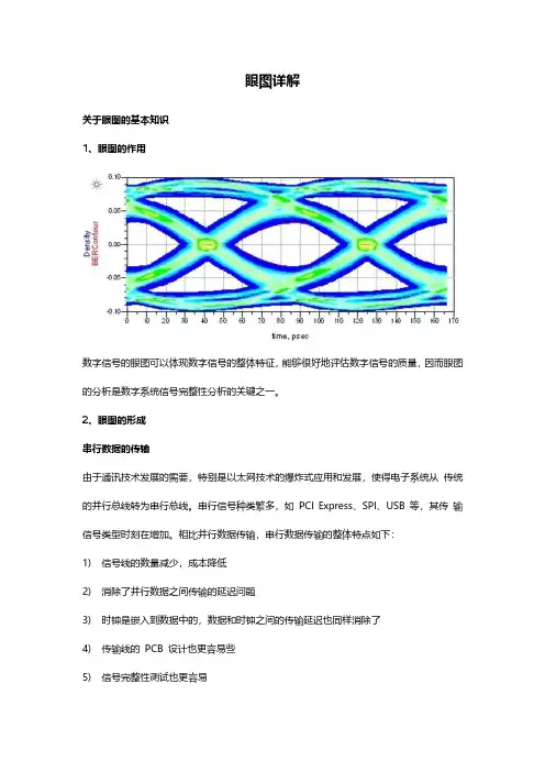
眼图详解关于眼图的基本知识1、眼图的作用数字信号的眼图可以体现数字信号的整体特征,能够很好地评估数字信号的质量,因而眼图的分析是数字系统信号完整性分析的关键之一。
2、眼图的形成串行数据的传输由于通讯技术发展的需要,特别是以太网技术的爆炸式应用和发展,使得电子系统从传统的并行总线转为串行总线。
串行信号种类繁多,如PCI Express、SPI、USB 等,其传输信号类型时刻在增加。
相比并行数据传输,串行数据传输的整体特点如下:1)信号线的数量减少,成本降低2)消除了并行数据之间传输的延迟问题3)时钟是嵌入到数据中的,数据和时钟之间的传输延迟也同样消除了4)传输线的PCB 设计也更容易些5)信号完整性测试也更容易实际中,描述串行数据的常用单位是波特率和UI,串行数据传输示例如下:串行数据传输示例例如,比特率为3.125Gb/s 的信号表示为每秒传送的数据比特位是3.125G 比特,对应的一个单位间隔即为1UI。
1UI表示一个比特位的宽度,它是波特率的倒数,即1UI=1/(3.125Gb/s)=320ps。
现在比较常见的串行信号码形是NRZ 码,因此在一般的情况下对于串行数据信号,我们的工作均是针对NRZ 码进行的。
由于示波器的余辉作用,将扫描所得的每一个码元波形重叠在一起,从而形成眼图。
眼图中包含了丰富的信息,从眼图上可以观察出码间串扰和噪声的影响,体现了数字信号整体的特征,从而可以估计系统优劣程度,因而眼图分析是高速互连系统信号完整性分析的核心。
另外也可以用此图形对接收滤波器的特性加以调整,以减小码间串扰,改善系统的传输性能。
眼图实际上就是数字信号的一系列不同二进制码按一定的规律在示波器屏幕上累积后的显示,简单地说,由于示波器具有余辉功能,只要将捕获的所有波形按每三个比特分别地叠加累积(如上图所示),从而就形成了眼图。
目前,一般均可以用示波器观测到信号的眼图,其具体的操作方法为:将示波器跨接在接收滤波器的输出端,然后调整示波器扫描周期,使示波器水平扫描周期与接收码元的周期同步,这时示波器屏幕上看到的图形就称为眼图。

基于眼动分析的玩具视觉感知形式研究1. 引言1.1 研究背景在当前快速发展的玩具市场中,越来越多的设计师和制造商开始意识到玩具的视觉感知形式对于用户体验的重要性。
传统的玩具设计往往只注重外观与功能,忽视了用户对于视觉感知的需求和反应。
如何利用科学的方法来研究玩具的视觉感知形式,以提升用户体验成为一个亟待解决的问题。
1.2 研究目的研究目的是通过眼动分析技术来探究玩具视觉感知形式的特点和规律,从而为玩具设计提供科学依据和指导。
通过研究玩具在用户眼睛注视过程中的注意点和注视路径,我们可以更准确地了解用户对玩具的视觉注意偏好,进而优化玩具的外观、色彩和形状设计。
通过分析不同用户群体在视觉感知上的差异,可以为不同年龄段和性别的用户提供个性化的玩具设计方案。
通过研究玩具的视觉感知形式,我们可以深入探讨玩具对儿童认知、情感和创造力发展的影响,从而推动玩具设计行业的创新和发展。
通过本研究,我们旨在探索眼动分析技术在玩具设计领域的应用潜力,为提升玩具的视觉吸引力和用户体验提供科学的方法和指导。
1.3 研究方法在本研究中,我们采用了眼动追踪技术作为主要研究方法,以探究玩具视觉感知形式与眼动行为之间的关系。
眼动追踪技术是通过追踪被试者眼睛的运动轨迹和注视点来获取视觉信息的一种有效手段。
通过这项技术,我们可以分析被试者在观察玩具时的注意力分布、注视时长、扫视路径等眼动参数,从而揭示玩具设计对用户注意力的影响。
本研究采用了实验方法,首先设计了实验方案,在实验中设定了一系列任务和情境,以引导被试者对玩具进行观察。
通过眼动追踪仪器记录被试者的眼动行为数据,我们可以详细了解被试者对不同类型玩具的视觉感知方式,为玩具设计提供依据。
除了眼动追踪技术,我们还将结合问卷调查、访谈等定性研究方法,以便综合分析实验结果,进一步探究玩具视觉感知形式对用户体验的影响。
通过多种研究方法的综合运用,我们将全面而深入地探讨基于眼动分析的玩具视觉感知形式研究。
一文看懂数字定时:时钟信号、抖动、迟滞和眼图通过本文可以了解时钟信号的数字定时以及诸如抖动、漂移、上升时间、下降时间、稳定时间、迟滞和眼图等常用术语。
本教程是仪器基础教程系列的一部分。
1. 时钟信号发送数字信号其实发送的就是一串由0或1组成的数字序列。
然而,与不同设备进行通信时,定时信息要与发送的位相关联。
数字波形作为时钟信号的参考。
您可以将时钟信号看成是一个指挥者,它为数字电路系统的各个部分提供定时信号,使每个过程都可在精确的时间点触发。
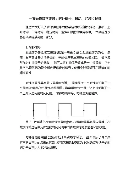
时钟信号是具有固定周期的方波。
周期是指一个时钟边沿到下一个同类时钟边沿之间的时间间隔,最常用的方式是一个上升沿到下一个上升沿之间的时间间隔。
时钟的频率等于时钟周期的倒数。
图1. 数字波形作为时钟信号的参考,时钟信号具有固定周期,在数据传输过程中用固定的时间间隔来同步数字信号发射器和接收器。
时钟信号的占空比是波形处于所占的时间比。
图2展示了两个具有不同占空比的波形的区别您可以发现占空比为30%的波形处于的时间少于占空比为50%的波形。
图2.信号的占空比是指波形处于的时间百分比。
时钟信号用于在数据传输过程中同步数字信号发射器和接收器。
比如,发射器可以在时钟信号的每个上升沿发送一个数据位,接收器可使用相同的时钟读取数据。
在这种情况下,设备的确定边沿是上升沿(从低电平到高电平)。
对于其他设备则可能是下降沿(从高电平到低电平)。
时钟的确定边沿又称为有效时钟边沿。
数字信号发射器在每个有效时钟边沿触发新的数据发送,而接收器则在每个有效时钟边沿上进行采样。
后来的设备开始同时使用时钟的上升验和下降沿;这种设备被称为双倍数据速率传输(DDR)设备。
事实上,数据传输对于有效边沿有短暂的短延;这种延时称为时钟到输出时间。
当接收器依据采集时钟接收数据时,我们需要注意两个定时参数,以确保接收数据的可靠性。
建立时间(ts)是指数据连续处于有效逻辑电平且接收器准备好接收输入信号所需的时间。
保持时间(tH)是指接收器采样后,数据发生变化前需要保持在原有状态的时间。
Agilent——眼图、抖动、相噪2009-02-25 22:31随着数据速率超过Gb/s水平,工程师必须能够识别和解决抖动问题。
抖动是在高速数据传输线中导致误码的定时噪声。
如果系统的数据速率提高,在几秒内测得的抖动幅度会大体不变,但在位周期的几分之一时间内测量时,它会随着数据速率成比例提高,进而导致误码。
新兴技术要求误码率(BER),亦即误码数量与传输的总码数之比,低于一万亿分之一(10-12)。
随着数据通信、总线和底板的数据速率提高,市场上已经出现许多不同的抖动检定技术,这些技术采用各种不同的实验室设备,包括实时数字示波器、取样时间间隔分析仪(TIA)、等时取样示波器、模拟相位检波器和误码率测试仪(BERT)。
为解决高数据速率上难以解决的抖动问题,工程师必需理解同步和异步网络中使用的各种抖动分析技术本文重点介绍3 Gb/s以上新兴技术的数据速率。
低于3 Gb/s的实时示波器可以捕获连续的数据流,可以同时在时域和频域中分析数据流;在更高的数据速率上,抖动分析要更具挑战性。
本文将从数字工程师的角度,介绍应对SONET/SDH挑战的各种经验。
抖动分析基本上包括比较抖动时钟信号和参考时钟信号。
参考时钟是一种单独的黄金标准时钟,或从数据中重建的时钟。
在高数据速率时,分析每个时钟的唯一技术是位检测和误码率测试;其它技术则采用某种取样技术。
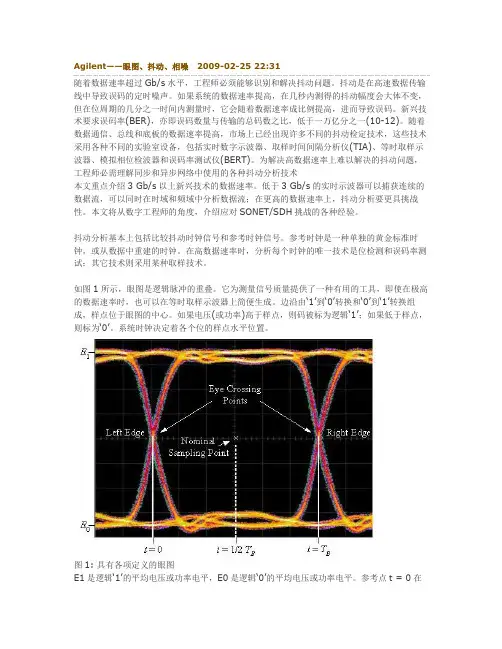
如图1所示,眼图是逻辑脉冲的重叠。
它为测量信号质量提供了一种有用的工具,即使在极高的数据速率时,也可以在等时取样示波器上简便生成。
边沿由‘1’到‘0’转换和‘0’到‘1’转换组成,样点位于眼图的中心。
如果电压(或功率)高于样点,则码被标为逻辑‘1’;如果低于样点,则标为‘0’。
系统时钟决定着各个位的样点水平位置。
图1: 具有各项定义的眼图E1是逻辑‘1’的平均电压或功率电平,E0是逻辑‘0’的平均电压或功率电平。
参考点t = 0在左边的交点进行选择,右边的交点及其后是位周期TB。

基于图像处理的眼动数据分析与应用研究眼动数据分析是一种重要的心理学和人机交互研究方法,通过分析被试者在观察图像过程中的眼部运动轨迹,可以了解他们在信息处理和注意力分配方面的模式与策略。
随着计算机视觉和图像处理技术的发展,眼动数据的分析可以借助图像处理方法进行更精确的定量分析,为人机交互系统的设计和改进提供有效的支持。
一、眼动数据的采集和处理1. 采集设备眼动数据的采集通常使用专业的眼动仪来完成。
现代的眼动仪具备高分辨率的摄像头和快速的数据采集系统,能够实时记录被试者的眼睛运动轨迹,并输出高精度的眼动数据。
2. 数据处理流程眼动数据的处理过程包括预处理、眼动事件检测和特征提取等步骤。
预处理阶段主要涉及眼动数据的滤波、矫正和同步等处理。
滤波可以去除误差数据,提高数据的质量;矫正是为了纠正因头部运动或眼动仪准确性等因素引起的数据偏移;同步是将眼动数据与其他生理信号或行为数据进行时间上的匹配。
眼动事件检测是分析眼动数据的核心任务,包括对注视点、扫视和眨眼等事件的识别和定位。
通过对眼动数据进行算法分析,可以实现自动化的事件检测,准确地提取目标事件的相关信息。
特征提取是对眼动数据的进一步分析,目的是从眼动数据中提取出与被试者的注意力、信息处理或认知行为相关的特征。
常用的特征包括注视点的空间分布、扫视路径的长度和速度、注视持续时间等。
二、基于图像处理的眼动数据分析方法1. 注视热点图注视热点图是一种常见的眼动数据可视化方法,可以将被试者的注视点分布情况以颜色强度的方式显示在图像上。
通常通过计算注视点在图像上的分布概率来生成注视热点图,可以直观地展示被试者在观察图像过程中的注意力分布。
2. 视觉注意模型视觉注意模型是模仿人类视觉注意机制构建的一种计算模型,能够模拟人类在观察图像时的注意力分配过程。
基于图像处理的视觉注意模型可以从图像特征的角度进行分析,通过计算图像的低级特征和高级特征来模拟被试者的视觉注意模式。

从眼状图入手,了解高电平抖动问题
要理解抖动,我们首先要了解眼状图。
眼状图是数字信号在时域中的表现形式,其中电压振幅按时间变化绘制。
一长串数据可分割成多个片段,称之为单位间隔(UI),这些UI 在示波器上一个个叠加,有助于示波器一次显示极大数量的数据。
单位间隔定义为UI = 1/比特速率。
如图 1 中眼状图所示。
一个眼状图由 1 个UI 组成(工程师有时会绘制两个并排眼状图),它是数字信号质量的视觉体现。
图1
既然我们了解了眼状图,就可提出这样一个问题“什幺是抖动?”抖动可定义为不希望看到的、信号理想转换位置的高频率偏移。
抖动可分为总体抖动(TJ)、随机抖动(RJ) 和确定性抖动(DJ)。
顾名思义,总体抖动(TJ) 包含所有抖动组成部分的影响。
下图 2 中的流程图是TJ 及其所有组件的分解图:
图2。

眼动数据分析与视觉注意力研究眼动数据分析是一种通过研究眼球在视觉任务中的运动轨迹来揭示人类视觉系统功能的方法。
视觉注意力是指个体在感知任务中对特定环境中某个特定部分的选择性关注和信息处理能力。
眼动数据分析与视觉注意力研究的目的是探索人类认知的机制和视觉注意力对信息处理的影响。
眼动数据分析的主要内容是通过眼动仪记录被试者在观察视觉刺激时的眼球运动,并对这些数据进行定量和定性分析。
眼动仪可以非常精确地测量被试者的注视点和视线轨迹,从而获得一系列眼动指标,如注视持续时间、注视频率和扫视速度等。
通过分析这些指标,可以揭示被试者在观察过程中的认知策略和注意分配。
眼动数据的分析可以用于不同领域的研究,如心理学、认知科学和人机交互等。
在认知心理学中,眼动数据被广泛应用于对注意机制、感知和记忆过程的研究。
例如,研究人员可以通过比较不同条件下的眼动数据来探索特定刺激对视觉注意力的影响。
在人机交互领域,眼动数据被用于评估用户对界面的注意分配和信息处理效率。
视觉注意力是个体在感知任务中对特定环境中某个特定部分的选择性关注和信息处理能力。
虽然我们的感知系统能够接收到大量的外界信息,但我们的注意力有限,只能关注特定的信息。
研究视觉注意力可以帮助我们了解人类是如何选择性地关注和处理信息的。
通过眼动数据的分析,研究人员可以研究视觉注意力在不同任务和情境中的变化。
在视觉注意力研究中,经常使用的实验范式是眼动定向搜索任务。
在这个任务中,被试者需要在一系列视觉刺激中寻找一个特定的目标。
研究人员可以通过分析眼动数据来了解被试者是如何选择注视点和扫视路径的。
例如,他们可以研究被试者在寻找目标时的注视点是否遵循一定的规律,比如是否更频繁地注视目标周围的区域。
通过这种方式,研究人员可以深入了解视觉注意力的机制和其对任务执行的影响。
除了眼动数据分析方法,近年来还出现了一些新的技术,如功能磁共振成像(fMRI)和脑电图(EEG),可以结合眼动数据来研究视觉注意力。
第一章绪论1.1研究背景人眼运动可以表证人的认知活动,而眼动追踪技术作为一种研究个体认知水平及心理状态的新型研究手段,被广泛地应用各个领域的基础研究和应用研究,为不同领域的研究者开展眼动追踪研究提供有价值的参考。
1.1.1眼动数据可视化的定义眼动数据可视化泛指一种专门通过使用各种眼神运动图像记录仪来进行实时图像、视频与各种眼动参数的记录,并运用各种方式将其转化为人们易于理解的图像或者其他形式。
视觉的立体感知过程开始于通过物体或周围情境所受的反射而发出来的黄色光线,然后阳光透过我们的眼角膜、瞳孔及其他晶状体而直接进入我们的整个眼睛。
视网膜上分布着两种不同的感光细胞:视杆细胞和视锥细胞。
按上述两种细胞的不同分布又将人类的视野范围分为三个主要区城:中央窝、旁中央窝和外围区城。
人眼主要通过旁中央窝来获取视觉信息,而该区域仅占整个视野范围的1%。
虽然只有很少部分,但此一个区域所记录的信息却包含了由视觉神经直接传递给人类大脑的有效视觉信息的50%。
虽然人眼的外围视野精度很差,但它更容易获得目标的运动和对比等信息,因此当我们把眼睛聚集到某个物体或者图片某个焦点时,生理上是将眼球的中央窝区城重合于我们眼球的晶状体当前的聚焦区域,这说明由于眼球的视觉特征,我们会将最多的视觉处理资源放在视野范围能获取最佳图像的特定区城,通过让中央窝区域获得图像,大脑才能够得到感兴趣区域的尽可能高的分辨率的图像和最多的视觉数据。
人类眼球的时间和空间采样能力限制了我们从周围环境中提取视觉信息的方式,当我们将视线从视野范围的中央区域移出时,视觉精度会迅速下降,所以需要使用一系列眼动行为使我们能够将视线放在目标物或场景的感兴趣的位置。
当我们头部保持静止观察静态物体时,我们主要的眼动行为是眼跳(Saccade)和注视(Fixation)。
但当我们在移动或物体在移动时,为了确保中央窝视野能够保持在感兴趣的位置就会触发其他的眼动行为,如集散运动(Distribution movement)能够帮我们将视线放在不同位置目标上,平稳跟踪(Smooth Pursuit)可帮助我们将视线放在运动的目标上,前庭眼反射(Vestibular ocular rellex)行为则能够在我们的头部或身体运动时将中央窝视野保持在兴趣点,所以眼动行为在我们处理视觉信息时起着关键的作用。
数字高清信号具有很高的数据率,为保证高清系统的建设安全,从系统设计到施工选材都要进行严格的测试和测量。
文章介绍了增强性测试、电缆长度增强性测试、SDI 校验场和CRC 误码测试,强调了利用眼图和抖动显示来帮助排查故障的重要性。
SDI 校验场信号 眼图 解调器法向高清晰度电视(HD )过渡可以是一个平稳的过程,当我们一开始对系统设备进行设计时,就应当严格按照正确的工程实践来进行。
对于数字高清信号,它具有很高的数据率,我们应当正确选用合适的电缆类型,这一点十分重要,同时还要确保施工质量。
在安装电缆的过程中应当避免对电缆施加外来的应力,例如扭转、弯曲等不正确的操作,这样就可以保证HD 信号能够很顺利地从A 点传送到B 点。
在施工过程中我们还要做一些简单的测试和测量,以保证每一传输链路段都具有良好的性能。
一 增强性测试在模拟传输系统中,信号的劣化是逐渐衰变的,但数字传输系统却有所不同,在信号崩溃之前它可以实现无故障工作。
到目前为止,还没有一种在线测试(服务中测试)方法可以测量传输系统的余量。
为了评估传输系统的运行状况,需要进行离线(中断服务)增强性测试。
在增强性测试中,可以改变数字信号的一项或多项参数直至出现传输失效。
导致信号传输失试时,我们可以按照有关串行数字视频标准(SMPTE 259M 或SMPTE 292M )来进行,最直观的测试方法就是增加电缆的长度直至错误发生。
其他测试方法有:改变信号的幅度或上升时间,或者在被测信号中插入噪声和(或)抖动等。
在这些测试方法中,每一种测试都可以用来评估接收机性能的一项或多项这种测试方法与SDI 校验场信号(该信号我们将在后文中予以介绍)结合起来,将是最有效的增强性测试,因为它可以反映系统的真实运行状况。
另一方面,我们在对接收机进行增强性测试时,如果所采用的测试方法只是检查接收机处理幅度变化的能力和插入抖动后的特性,虽然这种测试方法对于评估和验收设备是有用的,但是对于查看系统的运行状况却没有太大的意义(测量发送设备的信号幅度以及在系统中的各个部位进行抖动测量对于运行测试是重要的,但却不是增强性测试)。
抖动和眼图的视觉化分析抖动为实际数据与其理想位置的时间偏差TIE 为信号相对于标准时钟或者标准信号的定时误差TIE 在高速数字系统中即为抖动…0.0ns0.990ns 2.000ns 2.980ns 4.000nsP2P3P4P1TIE0.000ns-0.010ns0.000ns-0.020ns眼图是怎么形成的?Random Jitter(随机抖动)•随机抖动符合高斯型分布•直方图(估计) ↔ pdf(数学模型)•抖动峰峰值=无穷大…无界!1-sigma or RMS 7-sigma•内部热能现象•Flicker Noise, Shot Noise •热能的原子与分子振动•分子的解体•外部的宇宙射线Deterministic Jitter(确定性抖动)•确定性抖动是非高斯分布并且有界Peak-to-PeakPeriodic Jitter(周期性抖动)•TIE 随时间的变化是重复的、周期性的•Periodic jitter 和相位调制(PM)是等效的Peak-to-Peak•系统时钟(抖动频率在MHz 量级)•开关电源(抖动频率在KHz 量级)Duty Cycle distortion(占空比失真)•上升时间和下降时间不对称•或者测试时参考电平选择不当0.0v-0.1vInter-Symbol Interference(码间干扰抖动)•DDJ 或PDJ –数据相关性抖动或码型相关性抖动,和ISI的术语是等价的.•码型是如何影响随后的比特位的?◦由于传输链路的效应、反射等换个角度看抖动,时域看看我们有了什么视角?抖动视觉化–时间趋势图▪直方图告诉了我们分布,但是只有统计特性,缺少了时间信息▪时间趋势图可以直观告诉我们波形里是否有特定频率的调制▪下图为5个周期SSC @ 30khz抖动视觉化Gaussian Random Noise Sinusoidal Jitter抖动视觉化–频谱图▪从频域上观测抖动▪抖动中决定性的频率成分会在谱线上明显超出噪底哪个眼图好?哪个直方图好?视觉化眼图和抖动的问题?浴盆曲线误码率是关键vs. UI 张开程度•For a given position in the time there’s a given probability of error –“BER ”, Bit Error Ratio•For a given position in the time there’s a given probability of signal crossing –PDF , probability density function1 UIP r o b a b i l i t y o f ‘h i t ’P r o b a b i l i t y o f E r r o r –B E R基于示波器分析的浴盆曲线Rj δδ/Dj δδ与Tj @ BERAssume bi-modal distribution (dual-Dirac), measure Tj at two BER Fit curve to points, slope is Rj, Intercept is DjMeasuredTj @ 10-7MeasuredTj @ 10-4½Dj δδ½xRj δδEstimatedTj @ 10-12x≈7.4σx≈10.4σx≈14.1σ双狄拉克模型Conditions: only where Gaussian.抖动类型分析•抖动分离为误码产生的根本原因提供了更精确的定位和分析方法•抖动分析方法,参照T11 MJSQ ,已经被工业界广泛接受Constituent Components of Jitter= Unbounded= Bounded Total Jitter(TJ)Duty-Cycle Jitter (DCD)Data Dependent Jitter (DDJ)Periodic Jitter(PJ)Deterministic Jitter (DJ)Random Jitter(RJ)Jitter Visualization –Bathtub Plot▪Shows the Eye Opening at a Specified BER Level▪Note the eye closure of System I vs. System II due to the RJ-RJ is unbounded so the closure increases as BER level increases▪System I has .053UI of RJ with no PJ▪System II has .018UI of RJ and .14UI of PJ @ 5 and 10MhzSystem I System ISystem II System IITektronix -Innovators of Jitter Analysis •1998First Real-Time Scope Based Jitter Analysis Software•2002 Invented SW Based PLL Clock Recovery and the Spectral Approach for Jitter Separation•2004–Invented RT Eye rendering on a Real Time Scope•2004-First vendor to support both modeled (Dual-Dirac) and measured (Spectral) jitter methods •2005-Invented measurements with Jitter and Noise reconciliation•2011-First scope vendor with BUJ support•2015–RT Noise Analysis and Sampling BER and PDF Mask Testing抖动和眼图的视觉化眼图怎么切割的?时钟决定!TIE 抖动需要参考时钟•参考时钟提取的过程就是时钟恢复•参考时钟有几种确定的方式:◦Constant Clock with Minimum Mean Squared ErrorThis is the mathematically “ideal” clockBut, only applicable when post-processing a finite-length waveformBest for showing very-low-frequency effectsAlso shows very-low-frequency effects of scope’s timebase◦Phase Locked Loop (e.g. Golden PLL)Tracks low-frequency jitter (e.g. clock drift)Models “real world” clock recovery circuits very well◦Explicit ClockThe clock is not recovered, but is directly probed◦Explicit Clock (Subrate)The clock is directly probed, but must be multiplied up by some integral factorImportance of Clock Recovery•From spec, “The jitter measurement device shall comply with the JTF”.•How do I verify JTF?◦JTF is difference between input clock (ref) and input clock(unfiltered)◦Use 1100b or 0011b pattern (proper 50% transition density)◦Check 1) LF attenuation, 2) -3 dB corner frequency, and 3) slope23JTF vs PLL Loop Bandwidth•Configuring the correct PLL settings is key to correctmeasurements•Most standards have a reference/defined CR setup◦For example, USB 3.0 uses a Type II with JTF of 4.9Mhz•Type I PLL◦Type I PLL has 20dB of roll off per decade◦JTF and PLL Loop Bandwidth are Equal•Type 2 PLL◦Type II PLL has 40dB of roll off per decade◦JTF and PLL Loop Bandwidth are not Equal▪For example, USB 3.0 uses a Type 2 PLL with a JTF of 4.9Mhz.The corresponding loop bandwidth is 10.126 Mhz▪Setting the Loop Bandwidth as opposed to JTF will lead to24PLL Loop Bandwidth vs. Jitter Transfer Function(JTF)JTF Filtering Effects based on different PLL bandwidthsf3dB= 30 kHz f3dB= 300 kHz f3dB= 3 MHzJitter for Busy People Hints, Tips and Common ErrorsUsing the Jitter Analysis Tools•Issues manifested in different layers of theprotocol stack◦Crosstalk, jitter, reflections, skew◦Disparity, encoding or CRC errors•Where do I start debugging?•Jitter and Eye Diagram Tools◦Oscilloscope-based for quick results▪Fast jitter measurements with▫‘One Button’ Jitter Wizard▪Compare timing, jitter, eye, amplitude measurements▪User-definable clock recovery, filters, pass/fail limits, andreference levelsMore Hints for Successful Jitter Analysis•Clock Recovery has a great deal of influence on jitter results. Think about what you’re trying to accomplish.◦Constant-Clock is the most “unbiased”Often best if you’re trying to see very-low-frequency effectsBut it can also show wander in the scope’s timebase◦PLL recovery can model what a real data receiver will seeIt can track and remove low-frequency effects, allowing you to “see through” to the jitter that really contributes to eye closur e ◦Explicit-Clock is appropriate if your design uses a forwarded clockMake sure your probes are deskewedHints for looking at Spread-Spectrum Clock•If you don’t want to see the SSC effects, use TIE and PLL clock recovery with a bandwidth of at least 1 MHz. A Type-II (2nd-order) PLL will track out the SSC more effectively than a Type-I PLL.•If you do want to observe the SSC profile:◦Use a Period measurement and turn on a 3rd-order low-pass filter(in DPOJET) with abandwidth of 200 kHzBecause Period trends accentuate high frequency noise, the low-frequency SSC trend will be obscured if you don’t use a filter You can’t use a Frequency measurement directly. The combination of filtering and the reciprocal operation (Freq = 1/Per) cau se distortion in the resulting waveshape. (This is a mathematical fact, not a DPOJET defect.)◦If you use a TIE measurement, you’ll see modulation that looks like a sine wave. This is normal. It’s because TIE measures phase modulation, which is the integral of frequency. It turns out that the integral of a triangle wave looks very much like a sine wave.误码率与噪声分析Anatomy of a Serial Data LinkComplete LinkReceiverChannel+-+-+-+-+-+-+-+-E q u a l i z e rP r e -E m p h a s i sTransmitterAspirational goal: 0 errorsPractical Goal: Bit Error Rate < Target BER•Since BER is the ultimate goal, why not measure it directly?Serial Data Link Integrity = Bit Error Rate•Bit Error Ratio Testers (BERTs) are the tools for measuring BER directly •Why not use ONLY BERTs for Serial Data Link Analysis?◦Difficult to model/emulate equalizer◦Measurements could take a very long time◦Instruments are very expensive and not all that flexible◦Does not analyze the root causes of the impairments of the links•Alternative approach: use a scope and advanced analysis tools ◦Easily move from Compliance to Debug◦Better equipped to identify root causes of eye closure◦Equalizer can easily be modeled◦More cost effective◦Faster throughputWhy Measure Jitter and Noise?▪Link Model: Transmitter + Channel + Receiver▪Transmitter generates a stream of symbols▪Receiver uses a slicer to make a decision on the transmitted symbol▪The Bit Decision is made at a certain time (t) of the symbol interval and a comparison of the sliced data to a threshold (v) is performed ▪Jitter impairs the time slicing position▪Noise impairs the decision threshold?Jitter combined with Noise Analysis is a better predictor of BER performance!A Quick Look at Jitter and Noise Duality•Jitter analysis evaluates a waveform in the horizontal dimension based on when the waveform crosses a horizontal reference line.•Jitter decomposition is based on spectral analysis of Time Interval Error vs. time◦Individual jitter componentscan be separated (i.e.PJ, RJ, DDJ, etc.)◦TJ can then be estimated at atarget BER level ▪Noise evaluates along a vertical dimension on the basis ofcrossings of a vertical referenceline at some percentage of the unit interval (usually 50%).▪Noise decomposition is based on spectral analysis of voltage error vs. time–Individual noise components canbe separated (i.e. PN,RN, DDN, etc.)–TN can then be estimated at atarget BER level抖动和噪声的解析•Jitter and Noise Decomposition provide deep insight into BERFull Jitter Analysis vs. Mask Testing•Jitter separation analysis is able to extrapolate total jitter or eye closure at various Bit Error Rates at a specific voltage threshold but it doesn’t reveal the statistical eye closure at any other voltage.•Conventional mask testing considers both time and voltage , but cannot extrapolate eye closure at low BER.Can we combine the best of both?41Statistical Jitter + Noise Analysis•By jointly analyzing Jitter and Noise, behavior at all points in the eye can be extrapolated at low BER•The methodology is analogous to current jitter analysis, but is performed across both dimensions of the eye◦Jitter and noise are separated into components (Random, Periodic, Data-Dependent,…)◦The components are reassembled into a model that allows accurate extrapolation.42Timing-Induced Jitter•Since jitter is defined as a shift in an edge’s time relative to its expected position, it is easy to think of jitter as being caused by horizontal (chronological) displacement.•Note that the displaced edge (green) has not moved vertically in this example.43Noise-Induced Jitter•Consider a burst of voltage noise (right) that displaces a waveform vertically.◦In this case, the displaced edge (green) has not moved horizontally.•The jitter as measured at the chosen reference voltage is identical in these cases!◦So, why should we care?44Noise-to-Jitter (AM-to-PM) Conversion•Since waveform transitions are never instantaneous, the slope (slew rate) of the edge acts as a gain constant that controls how effectively noise is converted to “observed jitter”.•We can think of RJ as being composed of two components.◦Horizontally induced: RJ(h)◦Vertically induced: RJ(v)•Since these two components are uncorrelated with each other, they add in the RSS sense:RJ=RJ(h)2+RJ(v)2•Similarly, PJ can be decomposed into PJ(h) and PJ(v) based on root cause•We measure noise at a reference point in the bit interval (usually 50%)•If slew rate isn’t zero, jitter (horizontal displacement) causes observed noise•So as with RJ, RN can be decomposed into components:◦Horizontally induced: RN(h)◦Vertically induced: RN(v)•Similarly, PN can be decomposed into PN(h) and PN(v) based on root causeNoise to Jitter and Jitter to Noise ConversionConsider: an “ideal” edge in a patternactually has two impairments:◦Jitter(h) (see the blue trace)INTROD UCTION –and Noise(note that both of Jitter and Noise result in jitter on edge)The Combined response (bottomright) includes the jittercaused by noiseNon-impaired bit edgeWe can separate the noisecontribution of jitter for diagnosticpurposes by breaking RJ intoRJ(v) and RJ(h)DPOJET and 80SJNB are the only tool that will show you this separation, and thus give youan important troubleshooting hint: e.g. is it crosstalk causing trouble, or the clocks?48Theory: Construction of the BER Eye •Consider a very simple pattern: 7 bit repeating•Overlay multiple segments of the 7-bit pattern. Each one has noise and jitter, so although the bit pattern is clear, they follow many slightly different paths:•Average many pattern repeats together. Everything that is uncorrelated with the pattern averages out. What remains is called the ‘correlated waveform’.◦This waveform fully characterizes DDJ, DCD, DDN, ISI –all data dependent effects•The correlated waveform can be snipped into individual bits and overlaid to form an eye diagram, using the recovered clock as the alignment reference. This forms the ‘correlated eye’:•Spectral jitter separation is used to find PDFs of the random and periodic jitter.•The RJ and PJ PDFs are convolved to find the uncorrelated jitter PDF (red)• A similar analysis of the noise yields the uncorrelated noise PDF (blue)◦Care must be taken to properly account for AM-to-PM and PM-to-AM conversion in these steps; otherwise some noise or jitter would be ‘double-counted’.•Two-dimensional convolution is used to create a joint PDF of uncorrelated jitter + noise. (We can call this the ‘jitter/noise set’)•The jitter/noise set is convolved (two-dimensionally) with the correlated eye for the ‘1’ bits to get the overall(correlated + uncorrelated) PDF for ‘1’ bits•The ‘1’ bit PDF is integrated vertically (from bottom to top) to get the ‘1’ bit CDF (Cumulative Distribution Function)◦In this color-graded view, each color represents a particular BER level•A similar treatment for ‘0’ bits yields the ‘0’ bit CDF54Theory: Construction of the BER Eye –Conclusion•The ‘1’ bit and ‘0’ bit CDFs are added to get the overall “BER Eye”◦ A particular BER contour can be found in the 3D version of this plot by slicing it horizontally, or by extracting a specific color on either version◦Since this ‘eye’ looks rather unconventional, DPOJET extracts the3D ViewColor-Graded View。