实验8 反幂法

python 反幂运算-回复Python中的幂运算是计算一个数的指数次幂。

python提供了内置函数pow()和操作符来实现幂运算。

但是，本文将讨论如何进行反幂运算，即计算一个数的n次方根。

反幂运算是幂运算的逆过程，可以用来解决一些数学计算问题和科学工程问题。

在本文中，我们将一步一步地解释如何在Python中实现反幂运算。

步骤1：理解反幂运算的概念反幂运算是指找到一个数的n次方根的过程。

可以将其理解为通过给定一个数字n，计算一个数x，使得x的n次方等于给定的数字。

例如，对于给定的数字8和幂2，我们需要找到一个数x，使得x的平方等于8。

在这种情况下，x等于2，因为2的平方等于8。

步骤2：使用循环逼近方法一种常见的方法是使用循环逼近来计算反幂运算。

该方法基于一个简单的思想：从一个初始的猜测值开始，通过多次迭代来逼近最接近的数值。

在这种情况下，我们可以使用二分法来逼近。

步骤3：实现二分法逼近算法首先，我们需要定义一个函数来计算给定数字的反平方根。

在这个函数中，我们使用二分法来逼近最接近的数值。

def reverse_power(base, n, epsilon):low = 0.0high = baseguess = (low + high) / 2.0while abs(guessn - base) >= epsilon:if guessn > base:high = guesselse:low = guessguess = (low + high) / 2.0return guess在上面的代码中，我们定义了一个reverse_power()函数，该函数接受三个参数：base（基数）、n（次方）、epsilon（误差容限）。

在函数内部，我们初始化一个循环，直到我们的猜测结果接近给定的数字为止。

如果猜测的结果大于给定的数字，我们将高值更新为当前猜测结果；如果猜测的结果小于给定的数字，我们将低值更新为当前猜测结果。

幂法和反幂法的matlab实现幂法求矩阵主特征值及对应特征向量摘要矩阵特征值的数值算法，在科学和工程技术中很多问题在数学上都归结为矩阵的特征值问题，所以说研究利用数学软件解决求特征值的问题是非常必要的。

实际问题中，有时需要的并不是所有的特征根，而是最大最小的实特征根。

称模最大的特征根为主特征值。

幂法是一种计算矩阵主特征值（矩阵按模最大的特征值）及对应特征向量的迭代方法，它最大的优点是方法简单，特别适用于大型稀疏矩阵，但有时收敛速度很慢。

用java来编写算法。

这个程序主要分成了四个大部分：第一部分为将矩阵转化为线性方程组；第二部分为求特征向量的极大值；第三部分为求幂法函数块；第四部分为页面设计及事件处理。

其基本流程为幂法函数块通过调用将矩阵转化为线性方程组的方法，再经过一系列的验证和迭代得到结果。

关键字：主特征值；特征向量；线性方程组；幂法函数块POWER METHOD FOR FINDING THE EIGENVALUES AND CORRESPONDING EIGENVECTORS OF THEMATRIXABSTRACTNumerical algorithm for the eigenvalue of matrix, in science and engineering technology, alot of problems in mathematics are attributed matrix characteristic value problem, so that studies using mathematical software to solve the eigenvalue problem is very necessary. In practical problems, sometimes need not all eigenvalues, but the maximum and minimum eigenvalue of real. The characteristic value of the largest eigenvalue of the modulus maximum.Power method is a calculation of main features of the matrix values (matrix according to the characteristics of the largest value) and the corresponding eigenvector of iterative method. It is the biggest advantage is simple method, especially for large sparse matrix, but sometimes the convergence speed is very slow.Using java to write algorithms. This program is divided into three parts: the first part is the matrix is transformed into linear equations; the second part for the sake of feature vector of the maximum; the third part isthe exponentiation function block. The fourth part is the page design and eventprocessing .The basic process is a power law function block by calling the matrix is transformed into linear equations method, after a series of validation and iteration results.Power method for finding the eigenvalues and corresponding eigenvectors of the matrixKey words: Main eigenvalue; characteristic vector; linear equations; power function block、目录1幂法......................................................... . (1)1.1幂法的基本理论和推导 (1)1.2幂法算法的迭代向量规范化 (2)2概要设计........................................................ (3)2.1设计背景 (3)2.2运行流程........................................... . (3)2.3运行环境........................................... (3)3程序详细设计 (4)3.1矩阵转化为线性方程组……..………………………………………. .43.2特征向量的极大值 (4)3.3求幂法函数块............….....…………...…......…………………………3.4界面设计与事件处理..........................................................................4运行过程及结果................................................ (6)4.1 运行过程....................................... ..................………………………………………. .64.2 运行结果................................................ .. (6)4.3 结果分析.......................................... (6)5结论 (7)参考文献 (8)附录 (56)1 幂法设实矩阵nn ijaA ⨯=)(有一个完备的特征向量组，其特征值为n λλλ ,,21，相应的特征向量为nx x x ,,21。

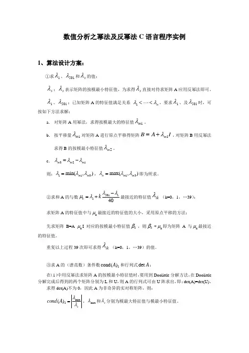
数值分析之幂法及反幂法C 语言程序实例1、算法设计方案：①求1λ、501λ和s λ的值：s λ：s λ表示矩阵的按模最小特征值，为求得s λ直接对待求矩阵A 应用反幂法即可。

1λ、501λ：已知矩阵A 的特征值满足关系 1n λλ<<，要求1λ、及501λ时，可按如下方法求解： a ． 对矩阵A 用幂法，求得按模最大的特征值1m λ。

b ． 按平移量1m λ对矩阵A 进行原点平移得矩阵1m BA I λ=+，对矩阵B 用反幂法求得B 的按模最小特征值2m λ。

c ． 321m m m λλλ=-则：113min(,)m m λλλ=，13max(,)n m m λλλ=即为所求。

②求和A 的与数5011140k k λλμλ-=+最接近的特征值ik λ（k=0，1，…39）：求矩阵A 的特征值中与k μ最接近的特征值的大小，采用原点平移的方法：先求矩阵 B=A-k μI 对应的按模最小特征值k β，则k β+k μ即为矩阵A 与k μ最接近的特征值。

重复以上过程39次即可求得ik λ（k=0，1，…39）的值。

③求A 的（谱范数）条件数2cond()A 和行列式det A ：在（1）中用反幂法求矩阵A 的按模最小特征值时，要用到Doolittle 分解方法，在Doolittle 分解完成后得到的两个矩阵分别为L 和U ，则A 的行列式可由U 阵求出，即：det(A)=det(U)。

求得det(A)不为0，因此A 为非奇异的实对称矩阵，则： max 2()scond A λλ=，max λ和s λ分别为模最大特征值与模最小特征值。

2、程序源代码：#include<stdio.h>#include<stdio.h>#include<math.h>#define N 501 //列#define M 5 //行#define R 2 //下带宽#define S 2 //上带宽#define K 39#define e 1.0e-12 //误差限float A[M][N]; //初始矩阵float u[N]; //初始向量float y[N],yy[N];float maximum,value1,value2,value_1,value_N,value_s,value_abs_max;const float b=0.16f,c=-0.064f;int max_sign,max_position;void Init_matrix_A() //初始化矩阵A{int i;for(i=2;i<N;i++){A[0][i]= c;}for(i=1;i<N;i++){A[1][i]= b;}for(i=0;i<N;i++){A[2][i]= (1.64-0.024*(i+1))*sin(0.2*(i+1))-0.64*exp(0.1/(i+1));}for(i=0;i<N-1;i++){A[3][i]= b;}for(i=0;i<N-2;i++){A[4][i]= c;}}void Init_u() //初始化迭代向量{int i;for(i=0;i<N;i++)u[i]=1.0;}void Get_max() //获得绝对值最大的数值的模{int i;max_position=0;maximum=fabs(u[0]);for(i=1;i<N;i++){if(maximum<fabs(u[i])){max_position=i;maximum=fabs(u[i]);}}if(u[max_position]<0)max_sign=-1;else max_sign=1;}void Get_y() //单位化迭代向量{int i;for(i=0;i<N;i++)y[i]=u[i]/maximum;}void Get_u() //获得新迭代向量{int i;u[0]=A[2][0]*y[0]+A[1][1]*y[1]+A[0][2]*y[2];u[1]=A[3][0]*y[0]+A[2][1]*y[1]+A[1][2]*y[2]+A[0][3]*y[3];u[N-2]=A[4][N-4]*y[N-4]+A[3][N-3]*y[N-3]+A[2][N-2]*y[N-2]+A[1][N-1]*y[N-1];u[N-1]=A[4][N-3]*y[N-3]+A[3][N-2]*y[N-2]+A[2][N-1]*y[N-1];for(i=2;i<N-2;i++)u[i]=A[4][i-2]*y[i-2]+A[3][i-1]*y[i-1]+A[2][i]*y[i]+A[1][i+1]*y[i+1]+A[0][i+2]*y[i+2]; }void Get_value() //获得迭代后特征值{value2=value1;value1=max_sign*u[max_position];}void Check_value() //幂法第二迭代格迭代{Init_u();Get_max();Get_y();Get_u();Get_value();while(1){Get_max();Get_y();Get_u();Get_value();if(fabs((value2-value1)/value1)<e)break;}}void The_value() //获取绝对值最大的特征值λ_501 {Check_value();value_abs_max=value1;}void The_Other_value() //获取特征值λ_1{int i;float value_temp=value1;for(i=0;i<N;i++){A[2][i]-=value_temp;}Check_value();value1+=value_temp;if(value1<value_temp){value_1=value1;value_N=value_temp;}else{value_N=value1;value_1=value_temp;}}int min(int a,int b) //两值中取最小{if(a<b)return a;elsereturn b;}int max(int a,int b) //两值中取最大{if(a<b)return b;elsereturn a;}void Resolve_LU(){int k,i,j,t;float temp;for(k=1;k<=N;k++){for(j=k;j<=min(k+S,N);j++){temp=0;for(t=max(max(1,k-R),j-S);t<=k-1;t++)temp+=A[k-t+S][t-1]*A[t-j+S][j-1];A[k-j+S][j-1]=A[k-j+S][j-1]-temp;}for(i=k+1;i<=min(k+R,N);i++){temp=0;for(t=max(max(1,i-R),k-S);t<=k-1;t++)temp+=A[i-t+S][t-1]*A[t-k+S][k-1];A[i-k+S][k-1]=(A[i-k+S][k-1]-temp)/A[S][k-1];}}}void Back_substitution()//方程组回代过程{int i,t;float temp=0;for(i=2;i<N+1;i++){for(t=max(1,i-R);t<i;t++)y[i-1]-=A[i-t+S][t-1]*y[t-1];}u[N-1]=y[N-1]/A[S][N-1];for(i=N-1;i>0;i--){temp=0;for(t=i+1;t<=min(i+S,N);t++)temp+=A[i-t+S][t-1]*u[t-1];u[i-1]=(y[i-1]-temp)/A[S][i-1];}}double Det_matrix() //求矩阵行列式值{int i;double det=1;Init_matrix_A();Resolve_LU();for(i=0;i<N;i++)det=det*A[2][i];return det;}float Get_norm() //获得迭代向量模{int i;float normal=0;for(i=0;i<N;i++)normal+=u[i]*u[i];normal=sqrt(normal);return normal;}void Get_yy(float normal) //迭代向量单位化{int i;for(i=0;i<N;i++){y[i]=u[i]/normal;yy[i]=y[i];}}void Get_value_s() //获得绝对值最小的特征值{int i;value2=value1;value1=0;for(i=0;i<N;i++)value1+=yy[i]*u[i];value1=1/value1;}void Value_min() //反幂法求绝对值最小的特征值{float norm=0;int count=0;value1=0,value2=0;Init_u();norm=Get_norm();Get_yy(norm);Back_substitution();Get_value_s();while(count<10000){count++;norm=Get_norm();Get_yy(norm);Back_substitution();Get_value_s();if(fabs((value2-value1)/value1)<e)break;}value_s=value1;}float Get_cond_A() //求矩阵条件数{float cond1;cond1=fabs(value_abs_max/value_s);return cond1;}void Value_translation_min() //偏移条件下反幂法求特征值{int i,k;float tr;for(k=1;k<K+1;k++){tr=value_1+k*(value_N-value_1)/40;Init_matrix_A();for(i=0;i<N;i++)A[2][i]-=tr;Resolve_LU();Value_min();value_s+=tr;printf("k=%d =>>>λi%d=%.13e\n",k,k,value_s);}}void main(){float cond;double value_det;printf("Contactme:****************\n");Init_matrix_A(); //初始化矩阵AThe_value(); //获取绝对值最大的特征值λ_501 The_Other_value(); //获取特征值λ_1printf("λ1=%.13e\n",value_1);printf("λ501=%.13e\n",value_N);value_det=Det_matrix(); //求矩阵行列式值Value_min(); //反幂法求绝对值最小的特征值printf("λs=%.13e\n",value_s);cond=Get_cond_A(); //求矩阵条件数Value_translation_min();//偏移条件下反幂法求特征值printf("cond_A=%.13e\n",cond);printf("value_det=%.13e\n",value_det);}3、程序运行结果：4、迭代初始向量的选取对计算结果的影响：本次计算实习求矩阵A的具有某些特征的特征值，主要用到的方法是幂法和反幂法，这两种方法从原理上看都是迭代法，因此迭代初始向量的选择对计算结果会产生一定影响，主要表现在收敛速度上。

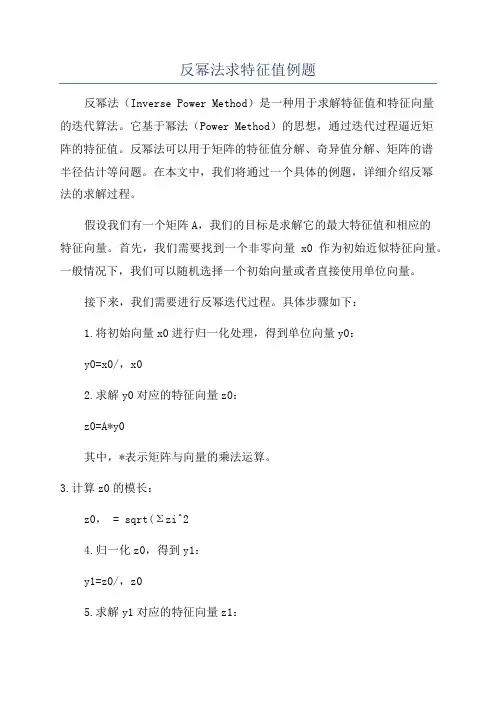
反幂法求特征值例题反幂法（Inverse Power Method）是一种用于求解特征值和特征向量的迭代算法。

它基于幂法（Power Method）的思想，通过迭代过程逼近矩阵的特征值。

反幂法可以用于矩阵的特征值分解、奇异值分解、矩阵的谱半径估计等问题。

在本文中，我们将通过一个具体的例题，详细介绍反幂法的求解过程。

假设我们有一个矩阵A，我们的目标是求解它的最大特征值和相应的特征向量。

首先，我们需要找到一个非零向量x0作为初始近似特征向量。

一般情况下，我们可以随机选择一个初始向量或者直接使用单位向量。

接下来，我们需要进行反幂迭代过程。

具体步骤如下：1.将初始向量x0进行归一化处理，得到单位向量y0：y0=x0/，x02.求解y0对应的特征向量z0：z0=A*y0其中，*表示矩阵与向量的乘法运算。

3.计算z0的模长：z0，= sqrt(Σzi^24.归一化z0，得到y1：y1=z0/，z05.求解y1对应的特征向量z1：z1=A*y16.重复步骤3-5，直到满足停止准则，如，λ(k)-λ(k-1)，<ε，其中λ(k)为第k次迭代求解的特征值。

例如，假设我们有如下矩阵A：210131014我们的目标是求解矩阵A的最大特征值和相应的特征向量。

首先，我们随机选择一个单位向量作为初始向量：x0=[1,0,0]^T归一化处理，得到y0：y0=[1,0,0]^T然后z0=A*y0=[2,1,0]^T接下来，计算z0的模长：z0， = sqrt(2^2 + 1^2 + 0^2) = sqrt(5归一化z0，得到y1：y1 = z0 / ，z0， = [2/sqrt(5), 1/sqrt(5), 0]^T然后，计算y1对应的特征向量z1：z1 = A * y1 = [3/sqrt(5), 7/sqrt(5), 1/sqrt(5)]^T重复上述步骤，直到满足停止准则。

假设我们设置停止准则为，λ(k)-λ(k-1)，<0.001、经过多次迭代，我们可以得到最终的近似特征值和特征向量。

矩阵的特征值与特征向量的计算摘要物理，力学，工程技术中的很多问题在数学上都归结于求矩阵特征值的问题，例如振动问题（桥梁的振动，机械的振动，电磁振动等）、物理学中某些临界值的确定问题以及理论物理中的一些问题。

矩阵特征值的计算在矩阵计算中是一个很重要的部分，本文使用幂法和反幂法分别求矩阵的按模最大，按模最小特征向量及对应的特征值。

幂法是一种计算矩阵主特征值的一种迭代法，它最大的优点是方法简单，对于稀疏矩阵比较合适，但有时收敛速度很慢。

其基本思想是任取一个非零的初始向量。

由所求矩阵构造一向量序列。

再通过所构造的向量序列求出特征值和特征向量。

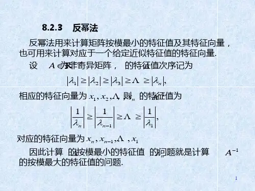
反幂法用来计算矩阵按模最小特征向量及其特征值，及计算对应于一个给定近似特征值的特征向量。

本文中主要使用反幂法计算一个矩阵的按模最小特征向量及其对应的特征值。

计算矩阵按模最小特征向量的基本思想是将其转化为求逆矩阵的按模最大特征向量。

然后通过这个按模最大的特征向量反推出原矩阵的按模最小特征向量。

关键词：矩阵；特征值；特征向量；冥法；反冥法THE CALCULATIONS OF EIGENVALUE AND EIGENVECTOR OF MATRIXABSTRACTPhysics, mechanics, engineering technology in a lot of problems in mathematics are attributed to matrix eigenvalue problem, such as vibration (vibration of the bridge, mechanical vibration, electromagnetic vibration, etc.) in physics, some critical values determine problems and theoretical physics in some of the problems. Matrix eigenvalue calculation is a very important part in matrix computation. In this paper, we use the power method and inverse power method to calculate the maximum of the matrix, according to the minimum characteristic vector and the corresponding characteristic value.Power method is an iterative method to calculate the eigenvalues of a matrix. It has the advantage that the method is simple and suitable for sparse matrices, but sometimes the convergence rate is very slow. The basic idea is to take a non - zero initial vector. Construct a vector sequence from the matrix of the matrix. Then the eigenvalues and eigenvectors are obtained by using the constructed vector sequence.The inverse power method is used to calculate the minimum feature vectors and their eigenvalues of the matrix, and to calculate the eigenvalues of the matrix. In this paper, we use the inverse power method to calculate the minimum eigenvalue of a matrix and its corresponding eigenvalues. The basic idea of calculating the minimum characteristic vector of a matrix is to transform it to the maximumc haracteristic vector of the modulus of the inverse matrix. Then, according to the model, the minimum feature vector of the original matrix is introduced.Key words: Matrix ；Eigenvalue ；Eigenvector ；Iteration methods;目录1引言 (1)2相关定理。

数值分析课程设计反幂法一、教学目标本节课的教学目标是让学生掌握反幂法的原理及其在数值分析中的应用。

知识目标要求学生了解反幂法的定义、性质及其在求解非线性方程中的应用；技能目标要求学生能够运用反幂法求解实际问题，并能够对结果进行分析和评价；情感态度价值观目标则是培养学生的探究精神、合作意识以及对于数学问题的兴趣。

二、教学内容本节课的教学内容主要包括反幂法的原理及其在数值分析中的应用。

首先，介绍反幂法的定义和性质，通过具体的例子让学生理解反幂法的含义和作用。

然后，讲解反幂法在求解非线性方程中的应用，并通过实际问题让学生掌握反幂法的具体操作步骤。

最后，对反幂法的优缺点进行总结，并引导学生思考如何选择合适的数值方法。

三、教学方法为了达到本节课的教学目标，将采用多种教学方法进行教学。

首先，运用讲授法为学生讲解反幂法的原理和性质，让学生掌握基本知识。

其次，通过讨论法让学生探讨反幂法在实际问题中的应用，培养学生的动手能力和解决问题的能力。

此外，还可以采用案例分析法和实验法，让学生在实际操作中感受反幂法的应用，并能够对其进行评价。

四、教学资源为了支持本节课的教学内容和教学方法的实施，将准备以下教学资源。

首先，教材和相关参考书，为学生提供理论知识的学习；其次，多媒体资料，包括PPT、视频等，用于直观展示反幂法的原理和应用；最后，实验设备，如计算机、计算器等，让学生能够在实际操作中掌握反幂法。

通过这些教学资源的使用，丰富学生的学习体验，提高学生的学习效果。

五、教学评估本节课的教学评估将采取多元化方式进行，以确保评估的客观性和公正性，并全面反映学生的学习成果。

评估方式包括平时表现、作业、小测验和期末考试。

平时表现主要评估学生的课堂参与度和提问回答情况；作业则是对学生掌握反幂法知识的检验，要求学生独立完成相关练习题；小测验则是在课程中期进行，用以检查学生对反幂法的理解和应用能力；期末考试则是对学生整个学期学习成果的全面考核，包括理论知识的理解和实际问题的解决。