Parasolid Geometry Modeling

ANSYS导入CAD二维模型的方法在ANSYS中，可以通过两种方法将CAD二维模型导入到软件中：直接导入和间接导入。

直接导入方法：1.打开ANSYS软件并创建新项目。

2. 点击“Geometry”选项卡下的“DesignModeler”进入建模环境。

3. 在设计模型器中，选择“File”选项，然后选择“Import”选择CAD文件。

4. 在弹出的文件浏览器中，浏览并选择要导入的CAD文件。

ANSYS支持多种CAD文件格式，例如IGES，STEP，Parasolid等。

5. 点击“Open”按钮导入CAD文件。

此时ANSYS会将CAD文件转换为ANSYS本地文件格式（.agdb或.gbx等）。

6. 在CAD文件转换完成后，可以选择将整个CAD文件导入ANSYS环境中，或选择导入文件的特定几何实体。

要导入整个CAD文件，请选择“Import Full Model”选项，要选择特定几何实体，请选择“Import Geometry”选项。

间接导入方法：1.将CAD文件导入到ANSYS支持的中间格式中，例如IGES，STEP等。

2.打开ANSYS软件并创建新项目。

3. 点击“Geometry”选项卡下的“DesignModeler”进入建模环境。

4. 在设计模型器中，选择“File”选项，然后选择“Import”选择中间格式文件。

5.在弹出的文件浏览器中，浏览并选择导入的中间格式文件。

6. 点击“Open”按钮导入中间格式文件。

7.此时，ANSYS将导入的文件转换为其本地文件格式，并在设计模型器中显示。

需要注意的是，CAD文件的复杂性和几何实体的数量可能会影响导入的时间和成功率。

在导入过程中，可能需要进行一些后处理操作来修复不完整或不正确的几何实体。

一些高级的CAD文件可能需要进行进一步的处理才能正确导入。

在处理过程中，根据具体情况可能需要进行不同的调整和优化。

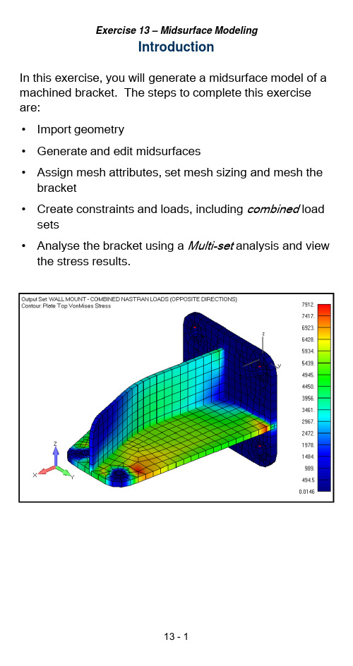
IntroductionIn this exercise, you will generate a midsurface model of a machined bracket. The steps to complete this exercise are:•Import geometry•Generate and edit midsurfaces•Assign mesh attributes, set mesh sizing and mesh the bracket•Create constraints and loads, including combined load sets•Analyse the bracket using a Multi-set analysis and view the stress results.Step 1:Import geometryImport the Parasolid geometry of the multi-thickness solid model.•Open a new FEMAP model.•Select the File, Import, Geometry command.•Select the Parasolid file ex13-Bracket_inches.x_t from your class Geometry folder.•Click OK to accept the defaults in the Solid Model Read Options dialog box.Change the view orientation to the Trimetric view.•Press the F8key (or use the View, Rotate, Model command) to open the View Rotate dialog box.•Select the Isometric button.•Click OK to close the dialog box.Save the model•Save the model in your class Exercises folder as “ex13-Bracket.modfem”.Step 2:Create midsurfacesExtract the midsurfaces from the solid.•Select the Geometry, Midsurface, Automaticcommand.•Click the Select All button to select all the surfaces on the solid.•In the Mid-Surface Tolerance dialog box, click the Measure Distance icon to enable measuring a 3-Ddistance. Ctrl+D can also be used to measure adistance from the graphics window while in acommand.•When the Locate –Define Location to Measure From dialog box is displayed, select one of the points onthe thickest edge of the sold. Set the Method to OnPoint and select one of the points shown below.•Click OK to confirm the selection of the first point.•Select the “other” point shown below that has not been chosen, then click OK to confirm the selection.•Click OK to accept the calculated distance, .156 in the Mid-Surface Tolerance dialog box. FEMAP willnow extract the mid-surfaces.Display the automatically generated Midsurfaces group.•In the Model Info pane, turn on “highlighting” by clicking the Show When Selected icon.•Expand the Group object in the tree and select1..Midsurfaces in the Model Info pane. This willhighlight the newly created group. Since we are onlyworking with a single part, you can delete the groupand the original solid.•Right-click 1..Midsurfaces and select Delete from the context-sensitive menu.•Expand the Geometry object in the Model Info tree, select 1..ex12-Bracket, and using the context-sensitive menu, Delete the original solid part.•Expand the view if needed with the Ctrl+A hotkey to “Autoscale”Note that the midsurfacing operation has generatedsplit lines in the midsurfaces that will be easily beremoved in the next step.Remove the split lines from the surfaces.•Select the command, Geometry, Solid, Cleanup.•Select All surfaces and click OK.•In the Solid Cleanup dialog box, accept the default option to Remove Redundant Surfaces and click OKto proceed with remove the split lines in the surfaces.Extend the surface representing the bend of the rib.•Switch your view orientation to the Front view.•Note that the bottom edge of bend surface doesnot intersect the surface representing the flange.•Select the command, Geometry, Midsurface, Extend.•Select the bottom edge of the bend surface in the Select Entity dialog box.Complete extending the surface representing the bend of the rib.•In the Surface Extend Options dialog box, leave the option for Extend Shape as Linear.•Using the Extend To –Solid option, select the Solid that represents the flange and click OK.Note that the blend surface now extends to theintersection with the flange.Trim the two surfaces representing the flat sections of the rib.You will use two different Geometry, Midsurfacecommands to do this, the first is to use the Trim with Curve operation and the second is use the Intersect operation.•Select the command, Geometry, Midsurface, Trim with Curve.•Select the flat surface of the rib closest to the back surface (the surface with the four mounting holes) inthe Solid/Surface to Trim dialog box and the clickOK.•In the Entity Select ion –Select Line(s) to Trim With dialog box, select the top edge of the rib and theedge of the blend surface intersecting the flat ribsection and click OK to confirm your selection.•With highlighting enabled in the Model Info pane, select the sheet solid of the rib section you justmodified and note how it has been sliced into threesurfaces.Continue with trimming the two surfaces representing the flat sections of the rib.•Select the command, Geometry, Midsurface, Intersect.•Select the two (2) surfaces that will represent the blend and the end of the rib then click OK togenerate the intersection.Delete the extraneous surfaces.•Select the command Delete, Geometry, Surfaces.•Select the small tab on the longer flat section of the rib and the two surfaces on the flat rib sections thatextend beyond the blend of the rib. Click OK todelete the surfaces.Stitch the surfaces together to create contiguous sheet solids.•Select the command Geometry, Solid, Stitch.•Select all the surfaces and click OK.•Click OK to accept the default Gap Tolerance.•Note how there are now three sheet solidsrepresenting the back face, web, and rib of thebracket.Intersect the surfaces to imprint the surfaces at the intersection of the three main features of the bracket.•Select the command Geometry, Midsurfaces, Intersect.•Select all the surfaces and click OK.•Again, using the Model Info pane, click the three sheet solids under the Geometry tree and note howthe surfaces have been imprinted using theintersection operation.Create Offset Curves around the six holes on thebracket.•If not displayed, active the Curves on Surfaces toolbar.•Click the Curve Washer icon on the Curves on Surfaces toolbar.•In the Define Washer or Offset Curves dialog box,set the Mode to Washer , enable the option for Save Split Lines and set the Offset to .125. Click OK to accept the settings.•Select one of the arcs on each of the six holes on thebracket and click OK .•Cancel out of the Curve Washer command.•After completing the Curve Washer operation, your model should appear as follows (shown with multiple windows to more clearly display the washers).Step 3:Assign mesh attributes, set mesh sizing and mesh the bracketAssign the mesh attributes (property) to themidsurfaces.•Select the Geometry, Midsurface, Assign Mesh Attributes command.•Press Select All the surfaces and click OK.•The Define Material –ISOTROPIC dialog box will open, prompting you for a material. Click the Loadbutton to open up the default material library.•In the Select from Library dialog box, select one of the Stainless Steel materials and click OK.•Click OK.•In the dialog box, click Yes to consolidate the properties by thickness.•Note that there are now two (2) properties that reflect the two different wall thicknesses of the part.Set the mesh size for the mid-surfaces.•Using the Select toolbar, set the Selector Entity to Surface and Selector Mode to Select Multiple .•Select all the surfaces by holding down the Shift keyto create a box picking region around the entire model.•In the graphics pane, right-click your mouse andselect Mesh Size from the context-sensitive menu.•In the Automatic Mesh Sizing dialog box, set the Element Size to .2 set the Max Angle Tolerance to15. Disable the Max Elem on Small Feature optionthen click OK to set the mesh size.Set the mesh size for the curves around the holes•Before meshing, turn on the mesh size indicators using the F6hotkey to open the View Options dialog box.•In the View Options dialog box, set the Category to Labels ,Entities and Color, enable the Draw Entityoption and set Show As to 3..Symbols and Count.Click Apply to update the display and once theoptions are displayed as below, you can close thedialog box by clicking either the OK or Cancelbutton.Set mesh sizes for the holes.•Using the Select toolbar, set the Selector Entity to Curve and leave the Selector Mode as SelectMultiple.•Select the curves surrounding the holes on the bracket to include the hole and the washer’s arcs,but not the split lines.•In the Model Info pane, expand the Selection List object .•Right-click the Curves object and select Mesh Size from the context-sensitive menu.•In the Mesh Size Along Curve dialog box, set the Number of Elements to 6 then click OK to set themesh size.Mesh the model.•In the Model Info pane, right –click the Surfaces object then select Mesh from the context-sensitivemenu.•Click OK in the Automesh Surfaces dialog box to mesh the model using the “Mesh Attributes”assigned to the surfaces in an earlier step.With mesh size symbols turned off and elementthickness display turned off, your model shouldappear similar to the following.Step 4:Create constraints and loads, including aCombined load setCreate the constraints on the back wall of the part.•In the Model Info pane, create a Constrain Set. Use a descriptive name for the title of the constraint set.•Expand the new constraint set and right-clickConstraint Definitions and select On Surface from the context-sensitive menu.•Select the eight (8) surfaces which represent the washers around the holes on the back wall of the bracket.•In the Create Constraints on Geometry dialog box,set the constraint to Pinned then click OK to create the constraints.•Again, right-click Constraint Definitions and select On Surface from the context-sensitive menu.Continue with creating the constraints on the back wall of the bracket.•Select the two (2) remaining surfaces on the back wall of the bracket and click OK.•In the Create Constraints on Geometry dialog box, set the constraint to Surface and choose Slidingalong Surface (Symmetry)then click OK to create the constraints.Create the loads on the holes on the left end of the bracket. To do this, you will create a Rigid elementconnecting the washers of the holes on the front of the bracket to a node at the center of the holes.•Select the command, Model, Element.•In the Define Plate Element dialog box, click the Type button an d select the Rigid element under theOther type.•Click the RBE2tab.•Click the New Node at Center button. Femap will then create the Independent node at the center ofthe selected Dependent nodes.•Click the Nodes button.•In the Entity Selection dialog box, change Methods^to on Curve and select the two curves making up one of the two holes on the web then Click OK to confirm your selection.•Create a second rigid element on the other hole byrepeating the previous two steps (New Node atCenter and selecting nodes on the two curves on the edge of the other hole).Create loads on the center nodes of the rigid “spider”elements in the holes.•Zoom in on the end of the bracket where you just created the rigid “spiders”.•From the Model Info tree, right-click the Loads object select New .•Enter a Title for the new Load Set as Front Web Hole Loading and click OK .•Expand the Load Set just created, right-click Load Definitions and select Nodal from the menu.•Select the node at the center of the front hole rigid element on the web then click OK .•In the Create Loads on Nodes dialog box, enter adescriptive name for the load, set the Load Type to Force , and set the Load value to FZ = 1.•Create a second load set and load at the node at the center of the read hole on the web by repeating steps b) through f) for the other hole. Set the Title for the second load set to Rear Web Hole Loading and click OK .Create a combined load set that will take the two previous load sets and by setting a scale factor, willcreate a combined load of 100 lbs in the negative Zdirection.•Select the command Model, Load, Combine.•In the Combine Load Data dialog box, set the Title to Combined 100 lb Web Hole Load.•In the From list, select both of the load sets you just created.•With both load sets selected, set the Scale Factor to -50.•Click the Add Combination button.•After the previous step, the Combinations section of the dialog box should appear as shown to the right.•Click OK to create the combined load set.•In the Model Info pane, right-click the combined load set you created and select Activate from the menu. Create a Nastran combined load set that will take the two previous load sets and by setting a scale factor, will create a combined load of 50 lbs in the positive Zdirection for the front hole and 50 lbs in the negative Z direction for the rear hole.•In the Model Info pane, right-click the Loads object and select New from the menu.•In the New Load Set dialog box, set the Title to a descriptive name similar to below.•For the Set Type, select Nastran LOAD Combination then click OK.•Select Reference Sets after right-clicking the newly created load set in the Model Info pane.•In the Referenced Loads Sets for Nastran LOAD dialog box, click the first load set under the Available Sets list field.•With the first load set selected, set the value For Referenced Set to 50then click the Add Referenced Set button.•With the second load set selected, set the value For Referenced Set to -50 then click the Add Referenced Set button. The Referenced Sets list field shouldappear as below.•Click OK to update the load set.Display the element thickness.•From the View toolbar, select the View Style pull down icon and select the Thickness/Cross Sectionicon to toggle on the display of the elementthickness.Step 5:Analyze the bracket and display stress resultsModify the Femap preference for Output Set Titles .•Select the command File, Preferences .•Select the Interfaces tab.•Under the Nastran Solver Write Options group, setthe Output Set Title option to 2..Nastran SUBTITLE .•Click OK to apply the changes to Femap’s preferences.Create an MultiSet Analysis Set and run the analysis.•Create an new analysis set for NX Nastran Linear Statics by right-clicking the Analysis object in theModel Info pane and select New.•Set the Title of the analysis set to MultiSet Linear Statics.•Expand the newly created analysis set to display Boundary Conditions.•Select Boundary Conditions then click Edit.Continue with creating the new analysis set for linear statics.•Set both the Constraints and Loads to None.•Click the MultiSet button.•In the Entity Selection –Select Constraint Set(s) to Generate Cases dialog box, click Select All thenOK.•In the Entity Selection –Select Load Set(s) to Generate Cases dialog box, click the Select fromList button.•In the Select One or More Load Sets(s) dialog box, select the two combined load sets, then clickOK.•Click OK to add the two load sets to the analysisset. The analysis set should now show two subcases as part of the analysis set.•Click the Analyze button in the Analysis Set Manager dialog box to start the analysis.•Close the NX Nastran Analysis Monitor when theanalysis completes and the results sets have been read into Femap.Review the results.•Activate the first results set by right-clicking on it in the Model Info pane.•Using the PostProcessing Toolbox, create a deformed contour plot of the Plate TopMajorPrin(cipal)Stress.•Set the Type to Elemental•Enable the option for Double-Sided Planar.•Save your model and exit Femap.。

为深入分析某轻型汽车车桥的桥体静态振动强度和车桥振动响应特性,运用新型有限元矢量分析法对它车桥进行矢量数值分析模拟。

采用一种有限元特性分析计算工具利用ANSYS对三种不同工况下的车桥结构进行了三种静态运动强度的特性分析,并对它们的三种动态强度特性分别进行了自由模态的特性分析。

应用有限数值单元运算法对它的数值进行运算模拟。

即:静力分析和动态分析中的网格可对局部进行加密,模态分析的数据良好，较为均匀，达到了理想程度。

从数据上看，静运动达到了合理水平，能够保证汽车车桥在设计时的性能要求。

通过数据分析实验结果明确表明,车桥主体结构的静运动特性和受力的变化特性基本都保证了车桥在设计中的一系列要求。

从而能够更好的设计车桥结构,并且让它具有好的静力特性和动态特性。

关键词:ANSYS，车桥，有限元，模态分析In order to deeply analyze the static vibration intensity and response characteristics of a light truck bridge, the new finite element vector analysis method is used to simulate its vehicle bridge. In this paper, a finite element analysis tool is used to analyze the characteristics of three kinds of static motion strength of vehicle bridge structure under three different working conditions by ANSYS, and the characteristics of three kinds of dynamic strength characteristics of them are analyzed by free mode. The finite element method is used to simulate its numerical value. That is to say, the mesh in static analysis and dynamic analysis can encrypt the local part, and the data of modal analysis is good and even, reaching the ideal degree. From the data point of view, the static motion has reached a reasonable level, which can ensure the performance requirements of the automobile axle in the design. Through the data analysis and experiment results, it is clear that the static and dynamic characteristics of the main structure of the axle and the changing characteristics of the force basically ensure a series of requirements in the design of the axle. So it can better design the axle structure, and make it have good static and dynamic characteristics.Key words：ANSYS, bridge, finite element, modal analysis前言 (1)1绪论 (2)1.1概述 (2)1.1.1国内外发展的状况及现状的介绍 (2)1.2 车型简介 (3)1.3 有限元方法简介 (3)1.3.1有限元法的基本原理 (3)1.4 ANSYS简介 (4)2车桥模型的建立 (5)2.1车桥单元类型的选取 (5)2.2 车桥模型的基本要求 (5)2.3 有限元建模方法的选择 (5)2.4模型简化 (6)3车桥静态分析 (7)3.1静态分析的基础 (7)3.2静力分析关系装配处理方法 (7)3.3操作台结构网格划分 (7)3.4边界条件与载荷的确定与施加 (8)3.4.1施加边界条件 (9)3.5分析和读取计算结果 (9)4车桥的模态分析 (10)4.1模态分析简介 (10)4.2模态的分析 (10)结论 (14)致谢 (15)参考文献 (16)附录 (17)有限元分析法在国内以及国外的汽车数值分析技术方面的运用和研究状况:有限元的单元运算法其实是一种很有效的汽车数值图形计算分析方法,它不仅能对帮助工程师在实际中发现几何体的形状不规则。

Geometric ModelingGeometric modeling is a crucial aspect of computer graphics and design, allowing for the creation of three-dimensional representations of objects and scenes. It involves the use of mathematical equations and algorithms to define the shape, size, and position of objects in a virtual space. Geometric modeling isused in a wide range of applications, including animation, video games, architectural design, and engineering. One of the key benefits of geometric modeling is its ability to create realistic and detailed representations of objects. By accurately defining the geometry of an object, designers can create lifelike images that closely resemble the real world. This level of detail is essential for applications such as architectural design, where precise measurements and proportions are crucial. In addition to creating realistic images, geometric modeling also allows for the manipulation and transformation of objects in a virtual space. Designers can easily modify the size, shape, and position of objects, allowing for quick iterations and adjustments during the design process. This flexibility is particularly valuable in fields such as industrial design and engineering, where multiple design iterations are common. Another important aspect of geometric modeling is its ability to simulate physical phenomena and interactions. By accurately modeling the geometry of objects andtheir relationships, designers can simulate how objects will behave in different environments and under various conditions. This is essential for applications such as virtual prototyping and simulation, where designers need to test the performance of a design before it is physically built. Geometric modeling also plays a crucial role in computer-aided design (CAD) and computer-aided manufacturing (CAM) processes. By accurately defining the geometry of objects, designers can create detailed blueprints and specifications that can be used to manufacture physical objects. This level of precision is essential for industries such as aerospace and automotive, where small errors in design can havesignificant consequences. Overall, geometric modeling is a powerful tool that enables designers and engineers to create realistic, detailed, and accurate representations of objects in a virtual space. By leveraging mathematicalequations and algorithms, designers can create lifelike images, manipulate objects,simulate physical interactions, and generate detailed specifications for manufacturing. As technology continues to advance, geometric modeling will continue to play a crucial role in a wide range of industries and applications.。

关于半挂车车架有限元分析与轻量化分析摘要：文章主要从半挂车实体建模及有限元的简述出发，分别简述了车架有限元模型的建立，以及轻量化的车架结构优化，旨在与广大同行共同探讨学习。

关键词：半挂车车架；有限元分析；轻量化一、半挂车实体建模及有限元的简述1.半挂车介绍半挂车是一种道路运输车辆，由两部分构成，一部分是带有动力的车头，另一部分为承载货物的半挂。

半挂车是目前普遍应用的运输工具，按用途分为专用和普通两种。

按大梁的结构来分有平板式、阶梯式、凹梁式三种。

如下图1-1所示。

图1-1 半挂车分类板式半挂车可以最大利用空间，同时离地面较高，方便公路运输。

阶梯式半挂车货台比较低，方便货物的装卸，凹梁式半挂车具有较小的离地间隙和较低的货台。

半挂车第二部分半挂结构主要由车架、双侧保护装置、工具箱、挡泥板、轮轴、牵引装置、电路、气制动、支撑、悬架装置、备胎、车箱、后保险杠等结构组成。

2.有限元法介绍有限元法是用简单的问题替换复杂的问题并进行求解，具有计算精度较高的优点，可对不同复杂形状的工程问题进行科学有效的分析以及计算。

二、车架有限元模型的建立建立有限元模型是进行有限元分析的基础，也即选择单元类型、赋予材料属性、划分网格、模拟连接方式、施加边界条件的过程，其中划分网格是前处理最为重要也是最为繁琐的步骤。

1.建立车架有限元模型应遵循的原则（1）确保模型的计算效率。

网格的大小、稀疏程度，也即单元与节点的数目多少，决定着计算结果的准确性和计算效率，在进行车架有限元模型建立的过程中应权衡好计算结果的准确性与计算效率的矛盾，找到最合适的网格尺寸。

（2）确保计算结果的准确性。

建立车架三维几何模型的过程中，在不影响分析结果的前提下，已经对车架进行了一定的简化，目的就是为了能够得到准确的结果，避免造成应力集中等问题。

2.模型导入及中面抽取（1）三维几何模型的导入和修复我们将利用 Solidworks 软件建立的车架的三维几何模型导入 Hypermesh 中。