2017年国际(美国)大学生数学建模竞赛获奖情况
- 格式:doc
- 大小:57.50 KB
- 文档页数:1

大学生数学建模竞赛简介全国大学生数学建模竞赛是由教育部高教司和中国工业与应用数学学会共同主办的面向所有大学生的全国性赛事,自1992年至今已举办了27届,目前成为全国高校规模最大、在国内外最具影响力的基础性学科竞赛,近年来逐渐吸引其他国家高校学生参赛。
全国大学生数学建模竞赛创办于1992年,每年一届,目前已成为全国高校规模最大的基础性学科竞赛,也是世界上规模最大的数学建模竞赛。
2017年,来自全国34个省/市/区(包括香港、澳门和台湾)及新加坡和澳大利亚的1418所院校/校区、36375个队(本科33062队、专科3313队)、近11万名大学生报名参加本项竞赛。
截止到2017年我校第十次组队参加全国大学生数学建模竞赛,在全体师生的共同努力下,取得了良好的成绩,共获得获得国家一等奖1项,国家二等奖2项,山东省一等奖20项、山东省二等奖21项,山东省三等奖5项,成功参赛奖40余项。
现对数学建模以及我校的组织工作做如下介绍,希望同学们能有所了解,可以从选报本学期的公共选修课《数学建模》开始,积极报名参加历年的全国大学生数学建模竞赛。
一、数学建模简介全国大学生数学建模竞赛是教育部高教司和中国工业与应用数学学会共同主办、面向全国高校所有专业大学生的一项通讯竞赛,从1992年开始,每年一届。
竞赛2007年开始被列入教育部质量工程首批资助的学科竞赛之一。
1.数学建模在科技、生产领域的重要性当需要从定量的角度分析和研究一个实际问题时,人们就要在深入调查研究、了解对象信息、作出简化假设、分析内在规律等工作的基础上,用数学的符号和语言,把它表述为数学式子(称为数学模型),然后用通过计算得到的模型结果来解释实际问题,并接受实际的检验。
这个全过程就称为数学建模。
近半个多世纪以来, 随着计算机技术的迅速发展,数学的应用不仅在工程技术、自然科学等领域发挥着越来越重要的作用, 而且以空前的广度和深度向经济、金融、生物、医学、环境、地质、人口、交通等新的领域渗透,所谓数学技术已经成为当代高新技术的重要组成部分。

美赛奖项等级引言美赛(美国大学生数学建模竞赛)是一项广泛知名的国际性竞赛活动,吸引了全球很多高校的学生参与。
在美赛中表现出色并获得奖项是许多参赛学生梦寐以求的目标。
本文将介绍美赛的奖项等级,并对获得不同奖项所需要的条件进行解析。
一、奖项等级简介美赛奖项等级按照参赛队伍的成绩划分,共分为五个等级,分别是:Outstanding(特别优秀奖),Finalist(决赛奖),Meritorious (优秀奖),Honorable Mention(荣誉奖)和Successful Participant(成功参与奖)。
这些奖项等级不仅代表了参赛队伍在比赛中的成绩,还彰显了他们在数学建模领域的能力与实力。
二、特别优秀奖(Outstanding)特别优秀奖是美赛中最高级别的奖项,获得这个奖项意味着队伍在比赛中表现出色、解决了较为困难的问题,并提出了富有创新性和实际可行性的解决方案。
通常,特别优秀奖只会授予少数参赛队伍,因此获得这个奖项是非常具有荣誉感和挑战性的。
三、决赛奖(Finalist)决赛奖是美赛中第二高级别的奖项,获得这个奖项的队伍在比赛中取得了显著的成绩,提出了创新的数学模型并解决了复杂的问题。
但与特别优秀奖相比,决赛奖的数量相对较多,所以获得这个奖项的机会相对较高。
四、优秀奖(Meritorious)优秀奖是美赛中的第三个等级,获得这个奖项的队伍在比赛中展现出了较为扎实的数学建模能力。
他们所提出的解决方案可能不如决赛奖和特别优秀奖的队伍那样创新,但仍然能够解决问题并给出合理的结论。
优秀奖是一种对参赛队伍能力的认可,也是绝大多数参赛队伍争取的目标。
五、荣誉奖(Honorable Mention)荣誉奖是美赛中的第四个等级,获得这个奖项的队伍在比赛中的表现相对一般,没有达到优秀奖的水平,但仍然能够解决问题并给出一定的结论。
荣誉奖的数量相对较多,对于一些刚开始参与美赛的团队来说,获得这个奖项也算是一种鼓励和肯定。
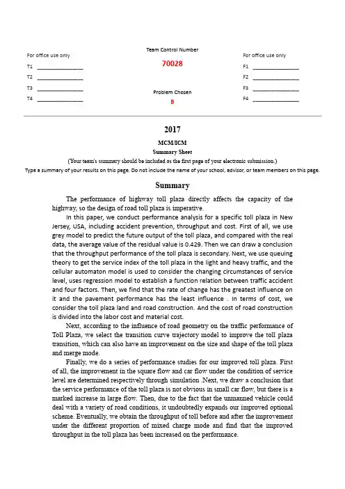
For office use onlyT1________________ T2________________ T3________________ T4________________ Team Control Number70028Problem ChosenBFor office use onlyF1________________F2________________F3________________F4________________2017MCM/ICMSummary Sheet(Your team's summary should be included as the first page of your electronic submission.)Type a summary of your results on this page. Do not include the name of your school, advisor, or team members on this page.SummaryThe performance of highway toll plaza directly affects the capacity of the highway, so the design of road toll plaza is imperative.In this paper, we conduct performance analysis for a specific toll plaza in New Jersey, USA, including accident prevention, throughput and cost. First of all, we usegrey model to predict the future output of the toll plaza, and compared with the realdata, the average value of the residual value is 0.429. Then we can draw a conclusionthat the throughput performance of the toll plaza is secondary. Next, we use queuingtheory to get the service index of the toll plaza in the light and heavy traffic, and thecellular automaton model is used to consider the changing circumstances of servicelevel, uses regression model to establish a function relation between traffic accidentand four factors. Then, we find that the rate of change has the greatest influence onit and the pavement performance has the least influence . In terms of cost, weconsider the toll plaza land and road construction. And the cost of road constructionis divided into the labor cost and material cost.Next, according to the influence of road geometry on the traffic performance of Toll Plaza, we select the transition curve trajectory model to improve the toll plazatransition, which can also have an improvement on the size and shape of the toll plazaand merge mode.Finally, we do a series of performance studies for our improved toll plaza. First of all, the improvement in the square flow and car flow under the condition of servicelevel are determined respectively through simulation .Next, we draw a conclusion thatthe service performance of the toll plaza is not obvious in small car flow, but there is amarked increase in large flow. Then, due to the fact that the unmanned vehicle coulddeal with a variety of road conditions, it undoubtedly expands our improved optionalscheme. Eventually, we obtain the throughput of toll before and after the improvementunder the different proportion of mixed charge mode and find that the improvedthroughput in the toll plaza has been increased on the performance.contents1 Introduction: (1)1.1 Problem background: (1)1.2 Steps: (1)1.3 Our work: (1)2 Assumptions (2)3 Nomenclature (2)4 Throughput analysis of grey forecasting model (3)5 error analysis (4)6 Service level of toll station (5)7 Vehicle lane changing rules based on Cellular Automata (6)8 Security analysis based on multivariate statistical regression mode (8)8.1 Study on the rate of change of Toll Plaza (8)8.2 Study on the longitudinal slope of entrance section of Toll Plaza (9)8.3 Research on service level of toll station (10)8.4 Study on pavement performance of toll station (10)9 Safety performance evaluation model of toll station (11)10 Cost analysis model of toll station (11)11 Analysis of the influence of lane geometry parameters on its capacity (12)11.1 Determination of lane changing rate (12)11.2 Influence of geometric parameters on the flow of the car lane (14)11.3 Energy consumption analysis based on cellular automata model (15)Definition of energy consumption: (16)Numerical simulation and analysis of the results: (17)Influence of curvature radius on energy consumption (17)Influence of arc length on energy consumption (18)12 The effect of traffic flow on service performance based on improved queuing theory 1913 The influence of unmanned vehicles on the improved model of Toll Plaza .. 2114 The influence of charging method on improving model of Toll Plaza (21)15 Strengths and Weaknesses (22)15.1 Strengths: (22)15.2 Weaknesses: (22)15.3 Future Model Development: (22)Comprehensive improvement strategy of tollplaza1Introduction:1.1Problem background:Highway toll and toll plaza is to ensure traffic safety and unimpeded, however because of lack of unified design specification, toll station and its square construction exists many problems. Such as: low value because of the technical indicators to make square construction scale too small and cause the toll plaza opened only few years as the traffic bottleneck, and use the high value on the one hand, because of the technical indicators and make the toll station construction scale is too large, waste a lot of money and resources. Due to incorrect linear indicators, or too short, the gradual square square length is insufficient, square road centerline offset, etc., it is too difficult to use after the completion of the square.so establishing the toll gates and the toll plaza design norms, as soon as possible, has the very vital significance in standardizing the construction of the toll station, ensuring the smooth general characteristic of toll plaza and traffic safety, improving the charging efficiency and management level, reducing the land acquisition and controlling investment and so on .1.2Steps:·A performance analysis of any particular toll plaza design that may already be implemented through the following three factors: accident prevention, throughput and cost .·Determine if there are better solutions (shape, size, and merging pattern) than any in common use.·Consider the performance of your solution in light and heavy traffic.·Consider the situation where more autonomous (self-driving) vehicles are added and how the solution is affected by the proportions of conventional (human-staffed) tollbooths, exact-change (automated) tollbooths, and electronic toll collection booths (such as electronic toll collection via a transponder in the vehicle)1.3Our work:·Based on the available data ,we make a performance analysis of any particulartoll plaza design that may already be implemented .·According to the problem from the performance analysis ,we make out a better solutions (shape, size, and merging pattern) than any in common use.·Determine the performance of the solution in light and heavy traffic ,how the solution change as more autonomous (self-driving) vehicles are added to the traffic mix and how the solution is affected by the proportions of conventional (human-staffed) tollbooths, exact-change (automated) tollbooths, and electronic toll collection booths.2AssumptionsTo simplify the problem and make it convenient for us to simulate real-life conditions, we make the following basic assumptions.1. Each section of roads is one-way traffic2.Vehicles in the retention period of toll station can be neglected3.In any hour of the vehicle arrival rate is proportional to the length of time4.The probability of any vehicle arrival in one hour of time is not affected by the previous history .5. The vehicles arrive in line with the Poisson distribution, namely the headway is negative exponential distribution3Nomenclatureε(0)(t)the residual errorq(t)the relative errorc the variance ratioP the small error probabilityr the curvature of the bend radiusu the static friction coefficientl the gradual change ratiok the number of serving drivewayρ/k traffic intensityw mean time to stay at a toll stationd automotive braking distancef the tire and road surface friction coefficientY the number of traffic accidents in toll stations per year∆W Width of the gradualα1curve angle R 1the radius of convex curve points pdelay probability e(n,t) energy consumption of the first n vehicles from time t to t+14 Throughput analysis of grey forecasting modelFigure 4-0-1Schematic diagram of New Jersey toll plazaFirst of all, we chose a toll plaza on the New Jersey in the United States for a specific performance analysis of toll plaza, and it includes the accident prevention, throughput, and cost.In view of the throughput of the toll plaza, we choose the grey forecasting model GM(1,1) , to predict the throughput of the toll plaza. Due to the problem of uncertainty, so we take the grey prediction model to deal with it.Suppose x (0)(1),x (0)(2)…,x (0)(M )In order to overcome the irregular , we use accumulation processx (1)(t )=∑x (0)(i)M i<1 Such a relatively smooth new series approximation can be described by the following differential equation:dx (1)dt +ax (1)=μ Its an albino form discrete solution of differential equation is: x ̂(1)(i +1)=.x (1)−u a /e ;ai +u aThe type of the parameter a、u be determined by the least squares fitting method is as follows:(1)(2)(3)A ̂=0a u 1=(B T B);1B T Y N Among them the matrix is:B =[ −12,x (1)(1)+x (1)(2)-1−12,x (1)(2)+x (1)(3)-1⋯⋯−12,x (1)(m −1)+x (1)(m )-1] Y N =(x (0)(2),x (0)(3),⋯,x (0)(m ))TSo the original data fitting sequence is:x ̂(0)(1)=x (0)(1)x ̂(0)(i +1)=x (1)(i +1)−x (1)(i )Table 4-0-1 Traffic flow prediction table5 error analysisIn equation (11), and regulations, the original data of reducing value and its residual error and relative error between observed value is as follows{ε(0)(t )=x (0)(t )−x′(0)(t )q (t )=ε(0)(t )x (0)(t )×100%The following inspection of the accuracy: x(0)=1M ∑x (0)(t )M t<0 ε(0)=1M;1∑(ε(0)(t )−ε0M t<2)2Second, calculate the variance ratio c =s 2s 1and small error probability P =2|ε(0)(t )−ε(0)|<0.6745s 13(4)(5)(6) (7) (8) (9) (10) (11)Figure 5-0-2comparison chart of grey prediction modelWe use m、p、v max to represent quality of the vehicle, random delayprobability and maximum speed respectively, g represents the local acceleration of gravity, r represents curvature of the bend radius and u represents the static friction coefficient . With the road statistical analysis carried out on the real value and the error of predicted value, we obtain the following res ults:It shows that the GM(1,1)model prediction results have a better response to .reflect the actual situation.6 Service level of toll stationThe direct feeling of the driver to the traffic environment of the toll station is from the queue length of the toll lane, and the length of the queue depends on the service level of the toll station V/C. In this regard, we use the queuing theory model of multichannel Queuing service, in which the vehicle arrival time is in a Poisson distribution, which is the negative exponential distribution; Suppose m is random arrival rate ,c i is output rate,k is the number of serving driveway, ρ=m c .There is the probability of having no vehicle in the queuing theoryρ(0)=1,∑1n!k−1n=0p n :1k!ρk k k−ρ- Average number of vehicles in queueing theory:n =ρ+p n ρ(0)k!k n−k (1;ρk )2 (12)(13)queue length: q =n −ρ=p n ρ(0)k!k n−k (1;ρk )2 Average number of waiting vehicles per lanea =q kAverage waiting time in queue systems:d =n m =q m +1c Average waiting time in queue:W =q mMean tardinessDeceleration time of vehicle entering toll stationt 1=v 03.6a 1Mean time to stay at a toll stationw =E ,S -+W qVehicle acceleration time of leaving toll stationt 2=v 03.6a 2 In this equation, v 0 is the normal traffic flow (km/h); a 1 、a 2 are deceleration of the vehicle (m/s 2); W q is average queue time (s); E ,S - is expected service time (s);7 Vehicle lane changing rules based on CellularAutomataWe apply the previous cellular automata model, which is now extended to multi Lane case. The main difference between multi lane and single lane is to consider the model of lane changing. In this paper, we take 4 lanes as an example.In reality, it may be possible to change lanes when the driver is found to be close to the exit and the front of the adjacent lane is empty. If you want to change lanes ,you should consider the vehicle behind the adjacent lane. When the distance (14)(15) (16) (17) (18) (19) (20)to the rear of the adjacent lane reaches to a certain length, you can change the road. Lane change scenarios can be shown in figure (), when the c car on the 1 Lane is blocked by the c 1 car, while the c 2 and c 3 cars on the 2 lanes are relatively large. in order to maintain the speed, c car will change to the road lane 2.Figure 7-0-3Schematic diagram of lane changingWhether or not the driver chooses the lane change is mainly decided by the d 0,d n,otℎer 、d n ,back three indicators, through the previous research, this paper thinks that the lane changing rule is:When d n,back >v maxC n ={1−C n d n <min{v n +1,v max } d n,otℎer >d n ,d n,back >v max c n Otℎer circumstancesWhen d n,back ≤v max ,C n ={1−C n d n <min{v n +1,v max } d n,otℎer >d nv max −θ(−∆x )α>1+min{d n,otℎer +1,v max }−min *V n +1,v max +c n Otℎer circumstancesAmong them, C n is the n car in the lane , C n =0 or 1,d n 、d n,otℎer andd n,back are the distance between the first n vehicle and the front vehicle, the distance from the adjacent lane and the distance from the vehicle in the adjacent lane, respectively. d safe is safety lane change model.d n,back −v max , ∆x <0, v max −θ(−∆x )α is the distance between the vehicle and the vehicle in the adjacent lane after correction by the value function, 1+min{d n,otℎer +1,v max }−min *V n +1,v max + is Limit Lane distance. The parameters α and θchange according to the psychological status of driver. If α>1, the greater α is, the more careful the driver is. If θ>1, the greater θis, the more careful the driver is. When α=1,θ=1,that ’s Lane changing model.(21) (22)In order to discuss the αandθ, we use Cellular automata simulation. In a two lane road with a length of7.5km, adopting the open boundary condition, each lane is composed of 1000cells with a length of7.5km, the maximum speed of vehicle v max=5. The random slowing down rate was 0.2.8Security analysis based on multivariate statistical regression modeAimed at the prevention of the accident, we use multiple linear regression to establish a function between the number of traffic accidents and the following four factors: toll square gradient, service level, Toll plaza entrance section of the longitudinal slope, the Pavement performance of Toll station .Figure 8-1Cause analysis of accident8.1Study on the rate of change of Toll PlazaFan in and fan out area of toll plaza are designed to make the gradual vehicles more natural smoothly in and out of the toll plaza. In order to drive vehicle easily , there has a requirement on its gentle gradient change. Otherwise the driver could produce driving deviation, which may cause improper operation and endangers safety.The relationship is as follow:(23)l=b,LAccording to the experience, the vehicles with straight into another lane deviation than at around 0.9m s⁄, drivers usually have no move feeling and uncomfortable feeling.Figure 8-1 The relationship between Accident number and Toll plaza ramp rateFigure 8-1 shows the relation curve between highway toll plaza ramp rate and traffic accident, the figure demonstrates that as the toll plaza ramp rate increases, the traffic accidents will increase, whereas the security of the toll plaza will decrease.Through the data regression analysis, we get the related models between toll plaza ramp rate and the number of traffic accidentsY =1.423e .0064xIn this equation, Y is the forecasted numbers of traffic accident corresponding to the toll plaza ramp rate , x is the toll plaza ramp rate of toll plaza.The correlation coefficient in the model R 2=0.8621, it shows that description model of correlation is higher, From the model ,we can learn that the occurrence of traffic accident frequency is proportional to the toll plaza ramp rate. Gradient length is insufficient, so it can't meet to slow down and change lanes entering the toll plaza vehicle safety requirements, resulting in the occurrence of traffic accidents .8.2 Study on the longitudinal slope of entrance section ofToll PlazaHighway toll entrance section of the longitudinal slope design without fully considering the characteristics of vehicles entering the toll plaza, a long downhill or turn downhill and so on bad road alignment, those will affect the normal operation of the pilot and make the vehicles entering the toll plaza slowdown not sufficient, longitudinal safe driving distance not enough and driving direction can't adjust to the charge lane ,which will causetraffic accidents. This will lead to serious losses. (24)Figure 8-0-4 entrance section of the longitudinal slope and accident numberThrough regression analysis, we get the relevant model between the toll plaza entrance section of longitudinal wave and traffic accidentsY =2.6254e 0.638xIn this equation, Y is the forecasted numbers of traffic accident corresponding to the toll plaza ramp rate , x is the longitudinal wave of t oll plaza’s entry section .The correlation coefficient in the model R 2=0.9219,it shows the correlation of this model is relatively high. But we can learn that toll station ‘s traffic accident and its entrance section of longitudinal wave have a positive correlation from figure model representation ,.The greater the slope, the lower charge war security.8.3 Research on service level of toll stationBased on the previous research of service performance of toll station, we take V C as the measure of service level and Cite previous results. 8.4 Study on pavement performance of toll stationAccording to the vehicle dynamics, the vehicle's braking distance can be expressed as follows:d =u 257.9(f:I) In this equation, d is automotive braking distance , u is the speed at the beginning of the automobile brake, f is the tire and road surface friction coefficient, Iis road longitudinal slope(25)9 Safety performance evaluation model of toll stationBased on the above analysis, the evaluation model of descriptive can be written as the equation form, using multiple linear regression model .Y is the number of traffic accidents in toll stations every year , x 1=1l ,x 2=V C ,x 3=i,则Y =β0+β1x 1+β2x 2+β3x 3N is sample size , Y i (i =1,2,…,N ) represent the Y value of sample i , x i 1,x i 2,…x i n (i =1,2…,N) represent the value of each variable insample I, respectively.令Y =[Y 1Y 2⋮Y n], X =[11⋮1x 11x 21⋮x n 1⋯⋯⋮⋯x 1n x 2n ⋮x n n ] β=[β0β1⋮βn ] Y =Xβ,making maximum likelihood estimate of each variable coefficient β1,β2,…βn , it can get a normal equations:X T Xβ=X T YSo you can get the following regression equationY =−4.4012−9.947511l +10.098V C +11.25i 10 Cost analysis model of toll stationWe selected the American New Jersey a toll plaza to make cost analysisFirstly, according to relevant data, we learn that New Jersey’s average price is (26) (27)(28)(29)(30)$3500 per mu,And the toll plaza which we analyzed occupies about 5 mu, therefore, the land price of the toll plaza is about $17500;Second, the road construction costs include labor and material cost, and the local construction industry ’s average monthly salary is $3000, we use it to calculate labor, this occupies the largest in the road construction costs; As for material cost, we calculate by the current prices in the United States, is about $40 per cubic meter, then according to the size of the toll plaza, it will cost about $45000.In conclusion, the cost of toll plaza spend mainly on the labor cost of highway construction, the material cost also accordingly account for part of it.11Analysis of the influence of lane geometry parameters on its capacity11.1Determination of lane changing rateAccording to the analysis of vehicle trajectory and running state of vehicle , vehicle trajectory in the middle of the gradual path is similar to vehicle lane changing trajectory, and considering the factors when the driver turns, we select the easement curve trajectory model to design the gradual change section of toll plaza. And in the middle of the two convex type curve , we join a long for L straight section , it is shown in the figure belowFigure 11-0-5Toll plaza improvementsAccording to characteristics of convex curve geometric elements, we can use the following formula to calculate the first period of convex curve of easement curve tangent length T1:T1=(R1+p1)tanα1+q1(31)2In this equation, R 1 is the radius of the first section of convex curve points , ρ1 is Within shift, q 1 is tangent increment, α1 is curve angle, and α1=2β1, β1 is easement curve angleSuppose the first and second convex curve gradient width are ∆W 1 and ∆W 2 respectively, the width of one side with the gradient is ∆W .Depending on the figure with the easement curve in orbit, there are: ∆W 1=T 1∙sin α1∆W 2=T 2∙sin α2∆W =∆W 1+∆W 2+Lsinα1∆W =0(R 1+p 1)(1−cos L S1R 1 )+q 11∙sin L S1R 1 +0(R 2+p 2)(1−cos L S2R 2)+q 21∙sin Ls2R 2 +Lsinα1 L S1 and L S2 are the length of easement curve of two convex curve respectivelyL is radial tangent of two convex curve, so α1=α2,then it Can be introduced as follows:L S1R 1 =L S2R 2 Associate (38) and (39),we can get the length of easement curve of two - Section convex curve L S1 and L S2, then the transition section longitudinal distance L y can use the following formula to calculate:L y =[(R 1+p 1)tan L S12R 1 +q 1+(R 2+p 2)tan L S22R 2 +q 2](1+cos L S1R 1 )+Lcosα1 Suppose the ramp rate of transition period is K ,then we can adopt the following equation:K =∆WL y From this equation , we can learn that the driving radius and the straight line segment L have a great influence on the length and the gradient of the gradient. The greater the radius, the longer the straight line, the longer the length of the gradient, the smaller the rate of change(32) (33) (34) (35) (36)(37)(38)11.2 I nfluence of geometric parameters on the flow of thecar laneAssuming C 0 and C 1=dC dl represent respectively bend and itsgradient , l represents the length of the curve itself , we can get C (l )=C 0+C 1lso ,the bend of the direction Angle isφ(l )=φ0+∫C(τ)l 0dτ=φ0+C 0l +12C 1l 2 The bend of the longitudinal distance x(l) and transverse distance y(l) are{x (l )=x 0+∫cosφ(τ)dτl 0y (l )=y 0+∫sinφ(τ)dτl 0 Assuming sinφ≈φ,cosφ≈1,and when x 0(l )=0,x (l )=l , then the bend of transverse distance y(x) and direction angle φ(x) can be expressed{φ(x )=φ0+C 0x +12C 1x 2y (x )=y 0+φl +12C 0x 2+16C 1l 3 Using the ideas of analytical mechanics, assuming that the longitudinal velocity along the x axis for x ′, along the y axis transverse speed for y ′ , along the z axis of horizontal pendulum angular velocity as the bits of ψ′, then from The Lagrange's equations we can get{ d dt .ðE T ðẋ/−ψðE T ðẏ=F Q 1d dt .ðE T ðẏ/+ψðE T ðẋ=F Q 2d dt .ðE T ðψ/+ẋ ðE T ðẏ−y ðE T ðẋ=F Q 3 Defining the system kinetic energy E T =12m (ẋ+ẏ)+12I z ψ2In the formula, m,I z respectively represent Vehicle quality and Rotary inertia take the derivative of (46),we can get{ d dt .ðE T ðẋ/−ψðE T ðẏ=d dt(mẋ)−ψ (mẏ)d dt .ðE T ðẏ/+ψðE T ðẋ=d dt (mẏ)−ψ (mẋ)d dt .ðE T ðψ/+ẋ ðE T ðẏ−y ðE T ðẋ=d dt (I z ψ)−x (mẏ)−y (mẋ) (39)(40)(41)(42)(43)Delimiting generalized force: {F Q 1=∑F xF Q 2=∑F y F Q 3=∑M zIn summary we can get the Vehicle longitudinal coupling model.We mainly consider the lateral situation∑F y =F yr +F xf +F xf cosδ If the vehicle driving in the bend is only disturbed by small disturbance near the equilibrium state, the front wheel angle is small enough , so cosδ≈1,sinδ≈δ ∑F y =−(C f +C r )y ẋ−(aC f −bC f )ψẋ+(F xf +C f )δ We put the formula () and formula () into ()y =−d 2ẏẋ−.ẋ+kd 3ẋ/ψ−(F xf :C f m )δ In the formula d 2=C f :C r m ,d 3=aC f ;bC rI z ,k =I z mThen, the resultant force ∑M z along the vertical direction is∑M z =aF xf sinδ+aF xf cosδ−bF yrWhen sinφ≈φ,cosφ≈1,then∑F y =−(a 2C f +b 2C r )ψẋ−(aC f −bC f )ẏẋ+a(F xf +C f )δψ=−d 4ψẋ−−d 3y ẋ+a I z (F xf :C f m )δ In the formula, d 4=(a 2C f :b 2C r )I z 11.3 E nergy consumption analysis based on cellularautomata modelConsidering the influence of different shapes on traffic performance is mainly reflected in the curve, we mainly study the influence of the curve on the whole problem. On the road segment, Lane set of sections containing only one plane curve, the curve is provided with the deceleration section of L , the road will be regarded as the length of the L 1D discrete lattice chain, each lattice point at each moment or is empty or occupied for a car.m 、p and v max represent the quality of the vehicle, the (44) (45)(46)(47) (48) (49) (50)(51)stochastic delay probability and maximum speed ,respectively, g is the local acceleration of gravity, r and u represent the static friction coefficient of curvature radius and static coefficient of friction between wheel and road, respectively. The vertical direction of the vehicle is subjected to a pair of balance forces, and the influence of tangential friction on the vehicle is mainly reflected in the change of the speed, Therefore , the centripetal force required for the safety of the vehicle is provided by the normal static friction force,v safe is maximum speed of safetyturning, then mv safe2r =μmg,⁄v safe =√μgr .In each step of t →t +1 , all vehicles are in accordance with the following rules of the evolution of the speed and location of the synchronization update :Determine the vehicle delay probability p :When the vehicle is in the buffer section , if v >v safe,take the probability of delay p =p 1 (larger), in other cases, take p =p 2 (smaller),Acceleration process: v n (t)→min (v n (t )+1,v max );deterministic deceleration process: v n (t)→min (v n (t ),gap n (t))Stochastic deceleration process with probability p :v n (t)→max (v n (t )−1,0) deceleration process :When the vehicle is in the corner of the road, and the speed v (t )>v safe , in order to turn the corner ,it must be slowed down :v n (t)→min (v n (t ),v safe )location update process: x n (t )→x n (t )+v n (t)Among them, v n (t) and x n (t ) are the speed and position of the first n vehicle at time t respectively , x n:1(t ) is the position of the first n +1 vehicle at time t . gap n (t )=x n:1(t )−x n (t )−1is the spacing between the first n car and the foregoing vehicle which is close to it.Definition of energy consumptionSuppose the mass of vehicle is m , when it slows down, its kinetic energy is reduced, we define the kinetic energy reduction for energy consumption, e(n,t) represents that energy consumption of the first n vehicles from time t to t+1 .e (n,t )={m,v 2(n,,t );v 2(n,,t:1)-2v (n,t )>v (n,t +1);0,v (n,t )≤v (n,t +1)The average energy consumption per vehicle per unit time:E d =1T 1N ∑∑e(n,t) N n<1t0:T;1t<t0 N is the total number of vehicles on the driveway, t 0 is relaxation time. For(52) (53)the energy consumption of the vehicle, if it is because the speed of t moment is greater than the Vehicle-to-vehicle distance v(n,t)>gap n(t), the vehicle decelerates, thatis defined as the interaction energy, denoted by E di; If it is because of the random deceleration caused, defined as the random deceleration energy consumption, denotedby E dr;if it is because the car speed In the corner v(n,t)>v safe, there is deceleration for the sake of driving safely, defined as safe energy consumption, denoted by E ds.Then total energy consumption is:E d=E di+E dr+E ds(54)Numerical simulation and analysis of the resultsTo simplify the problem, assuming that the length of actual road is 7.5km, Divided into 1000lattices, equivalent to the actual length of each grid correspondsto 7.5m, Delay probability p1=0.8,p2=0.25,Quality unit is defined 1. Entering probability changes from 0~1.0.The state of each vehicle is represented by its own speed v, v∈,0,v max-We let v max=5cell he actual speed is135km/h.We take8×104time steps every run .Influence of curvature radius on energy consumptionThe arc length s, the friction coefficient μand the radius of curvature of r are carried out numerical simulation. parameters are as follows: s=30m,μ=0.5,r=10、50、100、200、300m.According to v max=5cell/s,the maximum speed of the vehicle v max=37.5m/s. Results show that when r=300m, the safetyspeed v safe=√μgr=38.73m/s,v safe>v max, the bottleneck of the curve disappears and the speed limit is lost. The change of the probability in_p of therandom energy consumption(E di、E dr、E ds、E d)is shown in the figure.。
数学建模美赛数学建模美赛是一项由美国数学协会(MAA)、美国数学模型联盟(AMM)、美国数学教师协会(MCTA)和美国数学教育基金会(MEF)联合举办的国际数学建模竞赛。
它自1993年以来一直是一项年度数学建模竞赛,旨在激发学生的探索精神,培养学生的创新能力,促进学生的科学素养和思维能力,以及拓展学生的数学知识。
一、数学建模美赛的竞赛范围数学建模美赛的竞赛范围包括现代数学、应用数学、计算机科学、统计学、物理学、化学、生物学、社会学、经济学、工程学和其他科学领域。
竞赛任务要求参赛者使用数学建模的方法,对实际问题进行分析和把握,并以数学模型的形式提出解决方案。
二、数学建模美赛的参赛资格数学建模美赛的参赛者必须是高中生,可以是学校里的学生,也可以是家庭里的学生,只要他们的年龄在14-18岁之间。
参赛者可以单独参赛,也可以组队参赛,但每个团队最多只能有三名参赛者。
三、数学建模美赛的奖项设置数学建模美赛的奖项设置包括金牌、银牌、铜牌和优秀奖,其中金牌由最高分的参赛者获得,银牌由次高分的参赛者获得,铜牌由第三高分的参赛者获得,优秀奖由最具创新性的参赛者获得。
四、数学建模美赛的评审标准数学建模美赛的评审标准包括:模型的准确性、模型的创新性、模型的可行性、模型的可操作性、模型的可解释性、模型的可扩展性以及模型的可维护性。
五、数学建模美赛的参赛作品数学建模美赛的参赛作品包括:参赛者的模型报告、模型的计算结果、模型的结果分析、模型的可视化图表、模型的实际应用等。
参赛者需要根据竞赛任务,按照规定的格式提交参赛作品。
六、数学建模美赛的实施效果数学建模美赛的实施效果显著,它不仅激发了学生的探索精神,培养了学生的创新能力,促进了学生的科学素养和思维能力,拓展了学生的数学知识,而且还为学生提供了一个实现自我价值的平台,让他们有机会展示自己的才华。
七、数学建模美赛的未来发展数学建模美赛的未来发展前景一片光明。
数学建模美赛不仅将继续为学生提供一个实现自我价值的平台,而且还将不断推出新的数学建模竞赛,以更好地满足学生的学习需求,促进学生的科学素养和创新能力的发展。
关于“美国大学生数学建模竞赛”的组织管理办法一、赛事背景美国大学生数学建模竞赛(MCM/ICM,以下简称美赛),是唯一的国际性数学建模竞赛,也是世界范围内最具影响力的数学建模竞赛。
美赛始于1985年,由COMAP(the Consortium for Mathematics and Its Application,美国数学及其应用联合会)主办,得到了SIAM,NSA,INFORMS 等多个组织的赞助。
MCM/ICM 着重强调研究问题、解决方案的原创性、团队合作、交流以及结果的合理性。
竞赛以三人(本科生)为一组,在四天时间内,就指定的问题完成从建立模型、求解、验证到论文撰写的全部工作。
竞赛每年都吸引大量著名高校参赛。
20XX 年MCM/ICM 有超过7700支队伍参加,遍及五大洲。
MCM/ICM 已经成为最著名的国际大学生竞赛之一。
同济大学于20XX年首次组织学生参加该项赛事。
近年来,在学校领导关心指导下,在数学系数学建模指导教师团队的努力下,我校取得了令人瞩目的成绩,这不仅提高了同济大学的国际知名度,更为学校培养具有创新精神和竞争力的优秀人才、推动数学学科教学改革做出了一定的贡献。
为了更好的组织和管理美国大学生数学建模竞赛,特制定本办法。
二、组织参赛美赛由同济大学教务处主办,数学系承办以及负责具体指导工作,设立组织工作委员会和组委会秘书处,并指导数学建模协会工作。
三、竞赛奖励和学分认定1. 奖项设置美赛奖项设置如下:●Outstanding Winner 美赛特等奖(国内称法)●Finalist 美赛特等奖提名(国内称法)●Meritorious Winner 美赛一等奖(国内称法)●Honorable Mention 美赛二等奖(国内称法)●Successful Participant 成功参赛奖(国内称法)●Unsuccessful 不成功没有奖注:Finalist奖励给进入特等奖角逐未得到特等奖的队伍;Finalist 与Outstanding Winner全球一共约20支队伍。
MCM/ICM竞赛简介享有数学建模“奥林匹克”之称的MCM/ICM竞赛是一项面向世界各国大学生的国际性赛事,包括The Mathematical Contest in Modeling(数学建模竞赛)、The Interdisciplinary Contest in Modeling(交叉学科建模竞赛)和MCM/ICM Media Contest(数学建模媒体竞赛),由美国自然基金协会和美国数学及其应用联合会共同主办,运筹学与管理科学学会、工业与应用数学学会、数学学会等多家机构协办,目前已成为全世界最具影响力的大学生学科竞赛。
MCM(The Mathematical Contest in Modeling,数学建模竞赛)始于1985年,其宗旨是鼓励大学生通过对实际问题予以阐明、分析、建立数学模型并提出解法,来提高应用数学解决实际问题的能力和写作能力;ICM(The Interdisciplinary Contest in Modeling,交叉学科建模竞赛)始于2000年,其宗旨是发展并提升大学生运用数学方法解决交叉学科问题的能力和写作能力。
比赛每年举办一次。
竞赛形式为三名学生组成一队在四天内任选一题,完成该实际问题的数学建模的全过程,并就问题的重述、简化和假设及其合理性的论述、数学模型的建立和求解(及软件)、检验和改进、模型的优缺点及其可能的应用范围的自我评述等内容写出论文。
该项竞赛共设置四个奖项,分别为Outstanding Winner,Finalist,Meritorious Winner,Honorable Mentions。
在国内,约定俗成地将这四个奖项分别对应为特等奖、特等奖提名奖、一等奖、二等奖。
2013年吸引了来自中国、美国、加拿大、德国、印度、芬兰等15个国家和地区的6593支队伍参赛。
学习资料参赛规则【数学中国翻译】2014美国大学生数学建模竞赛(MCM/ICM)参赛规则中英文对照/thread-201325-1-1.html数学中国MCM/ICM参赛指南翻译(2014版)(任何单位转载须注明来源:)MCM:The Mathematical Contest in ModelingMCM:数学建模竞赛ICM:The InterdisciplinaryContest in ModelingICM:交叉学科建模竞赛ContestRules, Registration and Instructions比赛规则,比赛注册方式和参赛指南(All rules and instructions apply to both ICM and MCMcontests, exceptwhere otherwisenoted.)(所有MCM的说明和规则除特别说明以外都适用于ICM)To participate in a contest, each team must be sponsoredby a faculty advisor fromits institution.每个MCM的参赛队需有一名所在单位的指导教师负责。
美国(国际)大学生数学建模竞赛将于2015年2月5日-2月9日举行。
美国大学生数学建模竞赛(MCM/ICM),是唯一的国际性数学建模竞赛,也是世界范围内最具影响力的数学建模竞赛,为现今各类数学建模竞赛之鼻祖,目前我国已有清华大学、北京大学、浙江大学、上海交通大学、武汉大学等多所国内知名院校的学生参与了此项赛事的角逐。
2015年美国(国际)大学生数学建模竞赛比赛时间:美国东部时间:2015年2月5日(星期四)下午8点-2月9日下午8点(共4天)北京时间:2015年2月6日(星期五)上午9点-2月10日上午9点农历:十二月十八~十二月廿二重要说明:—COMAP是所有的规则和政策的最后仲裁者,对不遵循竞赛规则和程序的任何队伍,拥有唯一的自由裁量权,取消参赛资格或拒绝登记。
—评委、竞赛组织者、以及UMAP杂志的编辑拥有最终裁定权。
—如果参赛队伍违反竞赛规则,其指导老师一年内将不能指导其他团队,其所在参赛单位将被处以一年的察看处理。
—如果同一机构第二次被抓到违反规则的队伍,该学校将至少不被允许参加下一年度的赛事。
—以下所有时间都是美国东部时间EST(北京时间比美国东部时间早13个小时)—递交参赛论文后,意味参赛者同意以下条款:—论文提交后,出版权归COMAP,Inc所有;—COMAP可以使用,编辑,引用和出版论文,用于宣传或任何其他目的,包括在线展示,出版电子版,在UMAP杂志刊登或其他方式,并且没有任何形式的补偿;—COMAP可以在没有进一步的通知,许可,或补偿的情形下,使用这次比赛相关材料,团队成员、指导老师的名字,以及和他们的背景资料。
—递交参赛论文后,意味参赛者作出以下承诺:—论文中出现的所有的图像,数据,照片,图表,图画,如果未注明,都是由参赛者创建;如果引用其它资源,都在参考文献中列出,并在引用的具体位置标注来源。
—不论是直接,还是转述方式的文字引用,都在参考文献中列出,并在引用的具体位置标注来源;直接的文字引用使用引号标注。
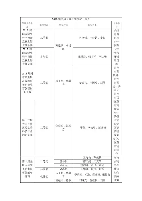
2015年学科竞赛获奖情况一览表学科竞赛名称 获奖等级 指导教师 获奖学生颁奖单位2015 国际大学生程序设计竞赛上海大都会赛 三等奖万建武、林逸峰林洛钊、王诗钧、李振美国计算机协会—国际大学生程序设计竞赛2015 国际大学生程序设计竞赛上海大都会赛参与奖 沈耀宗、张宇泽、李达峻2014常州市第五届高等教育和职业教育创新创业大赛 二等奖马正华、焦竹青姜成飞、王国瑞、刘静常州市科技局、常州市科协、共青团常州市委第十二届大学生物理及实验科技作品创新竞赛 二等奖包伯成、江兴方陆菱、李长頔、郑冰原江苏省高校大学生物理与实验创新竞赛组织委员会、江苏省物理学会第十届全国大学生飞思卡尔杯智能车竞赛 二等奖王诗钧、苏健鹏教育部高等学校自动化类专业教段仲麒邵天阔、江天皓何可人古剑锋、范迅、张硕三等奖 储志新 王朝轩、徐甫、杨循优胜奖朱正伟、焦竹青李长頔、柏凌、郑冰原、张超杰程起才、徐权刘继龙、倪成俊、刘让学指导委员会第六届“蓝桥杯”全国软件和信息技术专业人才大赛个人赛全国总决赛一等奖 杨亚南 林洛钊 中国软件行业协会、中国电子学会二等奖 杨亚南 王诗钧 王晖 李振 三等奖 高晋树 袁依洁 优秀奖 林逸峰 印佳奇 侯振杰 张超杰万建武 张宇泽第六届“蓝桥杯"全国软件和信息技术专业人才大赛个人赛江苏省赛一等奖王晖 林洛钊 侯振杰 王诗钧 王晖 李振 高晋树 袁依洁 朱家群 印佳奇 侯振杰 张超杰 万建武 张宇泽 二等奖朱家群 徐靖峰 杨亚南 曹童童 万建武 沈耀宗 杨亚南 耿勇强 苗林峰 向艳 曹景利 三等奖王晖 朱淳怡 高晋树 李彪 杨亚南杨洋向艳陈梦欣、顾榕晖、李敏荣、唐生平工业和信息化部人才交流中心 朱家群 徐竹西工业和信息化部人才交流中心 第四届“中国软二等奖 闫玉宝 陈永康、李振、王毓工业和信件杯”软件设计大赛息化部、教育部、江苏省人民政府2014年全国大学生电子设计竞赛 一等奖 贾鑫、曹松泽、范全有 全国大学生电子设计竞赛江苏赛区组委会 二等奖王将、何宝祥 朱庆之、胡钟昀、俞贵琴王将、陈墨 李长頔、郑冰原、陆菱刘继龙、刘让、赵紫嫣古剑峰、胡玉红、范迅何宝祥 杨循、徐甫、王杰2015年全国大学生数学建模竞赛 二等奖 王琼 郁秋华、汤俊伟、张进全国大学生建模竞赛组委会2015台达杯高校自动化设计大赛 一等奖 陈岚萍 周文涛 封晓鸣 邓开贵教育部高等学校自动化类专业教学指导委员会、中国自动化学会、工业与信息化职业教育教学指导委员会第二届全国高校物联网应用创新大赛 应用挑战赛决赛 一等奖 范伟伟、郇战 黄晓竹、宋文浩、刘志豪教育部科技发展中心、互联网应用创新开放平台联盟、清华大学软件学院第二届全国高校物联网应用创新大赛 编程挑战赛决赛 二等奖 李文杰、郇战 王胜、古剑峰、周浩成 三等奖 焦竹青 孙磊、贾鑫、耿宏杨第二届全国高校物联网应用创新大赛 应用挑战赛决赛 三等奖郇战 朱庆之、胡钟昀、杨瀚文潘操 刘东兵、曲继彬、陈江涛第二届全国高校物联网应用创新大赛 编程挑战赛华东赛区 一等奖焦竹青、郇战 孙磊、贾鑫、耿宏杨教育部科技发展中心、清华大学软件学院 范伟伟、郇战 黄晓竹、宋文浩、刘志豪教育部科技发展中心 二等奖李文杰、范伟伟徐晨、周浩成、王胜教育部科技发展中心、清华大学软件学院第二届全国高校物联网应用三等奖 郇战 陶亚辉、姜盼、王振海 教育部科技发三等奖 侯振杰 张建、陈永康、王建飞创新大赛 创意赛华东赛区展中心、互联网应用创新开放平台联盟、清华大学软件学院第二届全国高校物联网应用创新大赛 决赛 最佳指导教师奖郇战范伟伟第二届全国高校物联网应用创新大赛 三等奖侯振杰张建、陈永康、王建飞中国,清华大学软件学院,清华信息科技国家实验室 优秀奖 吴卓燃中国,清华大学软件学院,清华信息科技国家实验室全国高校互联网应用创新大赛 云计算 三等奖 庄丽华孙剑锋、周逸鸣、印佳奇、吴子琳教育部科技发展中心 、互联网应用创新开放平盟 江苏省物联网+大学生创新创业大赛创意组 二等奖何可人、诸燕平魏婷婷、刘森、陈伟、郭文卓江苏省教育厅2015全国大学生“西门子杯”工业自动化挑战赛 三等奖荆胜南周文涛、张凯莉、黄超教育部高等学校自动化类专业教学指导分委员会、西门子(中国)有限公司、中国系统仿真学会2015全国大学生“西门子杯”工业自动化挑战赛华东赛区二等奖 周文涛三等奖吕继东 邱钦、于莹、张浩张继 周园园、张凯莉、李宏哲2016年学科竞赛获奖一览表学科竞赛名称获奖等级 指导教师 获奖学生颁奖单位2016年”创青春”速度中国杯江苏省大学生创业大赛 银奖朱正伟刘鸿飞、王毓等 共青团江苏省委,省教育厅,省科技协会,省学联,省人银奖 张凯莉、白浩然等江苏省第二届“互联网+”大学生创新 银奖 朱正伟 刘鸿飞、王毓、张凯莉江苏省教育厅、省委宣传部创业大赛 一等奖 陈岚萍 杨小松、俞运柱、任佳俊 教育部高等学校自动化类专业教学指导委员会(清华大学代章)中国自动化学会、工业与信息化职业教育教学指导委员会自动化专业委员会 第三届台达杯高校自动化设计大赛 二等奖 陈岚萍 黄哲宇、刘乐天、翁逸飞2016中国工程机器人大赛暨国际公开赛 段锁林 殷聪聪、李大伟、朱方 教育部高等学校创新方法教导委员会、中国自动化学会机器人竞赛工作委员会、中国人工智能学会认知计算与信息处理专业委员会、国际工程机器人联盟、中国工程机器人大赛暨国际公开赛中国大学生计算机设计大赛 三等奖 侯振杰 李维康、朱亚洲、张幼安 教育部高等学校计算机类专业教学指导委2016年(第9届)中国大学生计算机设计大赛 二等奖 江兴方 王浩教育部高等学校计算机类专业教学指导委员会,等常州市第六届高等教育和职业教育创新大赛 二等奖 侯振杰 李维康、陈永康常州市教育局国家级大学生创新创业训练计划项目 结项 邹凌、周天彤李振、王诗钧、林洛钊、苏健鹏江苏省教育厅高教处 结项 邹凌、吕继东焦鼎、张旖帆、古剑锋、封景、林洛钊江苏省大学生创新创业训练计划项目 结项 庄丽华、李宁 印佳奇、孙剑锋、周逸鸣、夏春天“中关村青年杯”第十二届全国研究生数学建模竞赛 二等奖 宋文浩 教育部学位与研究生教育发展中心、全国研究生数学建模竞赛组委会、北京交通大学 二等奖 郭晓二等奖 刁小敏三等奖 汪伟昕三等奖 马凯三等奖 贺小捧二零一五年高教社杯全国大学生数学建模竞赛(本科组) 一等奖建模教练组袁桥、仝志方、任彦全国大学生数学建二等奖 王玺、王冠球、周亚文二等奖 陆青云、施佳瑜、李达峻二等奖 朱文浩、徐菁茹、程小雪 模竞赛组织委员会 二等奖 林振兴、鲍伟杰、李咏维 二等奖 郁秋华、汤俊伟、张进“华为杯”第十三届全国研究生数学建模竞赛一等奖 徐明华等 刘晨 教育部学位与研究生教育发展中心、全国研究生数学建模竞赛组委会、重庆大学一等奖 宋丽萍 一等奖 祝磊 二等奖 王凯 二等奖糜超专项奖 刘晨、宋丽萍、祝磊全国大学生数学建模竞赛 一等奖 建模教练组张建、吴卓然、朱淳怡 全国大学生数学建模竞赛江苏赛区组织委员会、中国工业与应用数学学会 二等奖 常宇、张新伟、朱云鹏 二等奖 朱瑾、朱磊、傅新康 二等奖周颖、相国林、陈曦三等奖 王行远、陈泽旭、范玲玲全国大学生数学建模 二等奖江兴方、王琼、张英丽郁秋华、汤俊伟、张进 教育部高等教育司 中国工业与应学学会2015指导第四届“认证杯”数学中国数学建模国际赛(小美赛)二等奖( ) 二等奖 姜忠义 张金鑫,陈佳丽,王宏林内蒙古自治区数学学会和全球数学建模能力认证中心2016美国大学生数学建模竞赛()二等奖( ) 二等奖 姜忠义 鲍伟杰,林振兴,李咏维美国数学及其应用联合会主办2016年美国大学生数学建模竞赛 三等奖吴春青 常宇 张新伟 朱云鹏美国数学及其应用联合会一等奖王世飞 周颖、万根、向国林美国数学及其应用联合会主办数学建模小美赛 成功参赛奖王世飞 蒋永杰、罗康英、徐亚男内蒙古自治区数学学会2016全国大学生数学建模竞赛 二等奖 姜忠义,徐月华,张洪波刘雪芹,王彬,王赟中国工业与应用数会二等奖 姜忠义,王世飞,徐明华王凯,江亚宁,糜超教育部学位与研究生教育发展中心江苏省普通高等学校第十三届高等数学竞赛 一等奖 赵志新,石澄贤 蒋雨恒江苏省教育厅江苏省普通高等学校第十三届高等数学竞赛组委会江苏省高等学校数学教学研究会江苏省普通高等学校第十三届高等数学竞赛 三等奖 赵志新,石澄贤田雪玫、袁 乔、汪明轩、叶志峰、邹 威第二届全国高校物联网应用创新大赛三等奖郇战胡钟昀、朱庆之、杨翰文教育部科技发展中心、互联网应用创新开放平台联盟、清华最佳指导教师奖二等奖 李文杰、郇战 王胜、古剑峰、周浩成一等奖 范伟伟、郇战 黄晓竹、刘志豪、宋文浩软件学院2015年全国大学生电子设计竞赛 江苏赛区二等奖 王天成、郇战 刘继龙、刘让、赵紫嫣全国大学生电子设计竞赛江苏赛区组委会 2016年杯江苏省大学生电子设计竞赛一等奖袁斌、武花干刘康平、马海二等奖 储开斌、朱正伟 朱金鑫、唐安昊、刘玉喜 二等奖 王天成、储志新 李海洋、崔建凯、汤沁怡二等奖武花干、王将钟欣辰、张硕、陈宏宇 二等奖 何宝祥、郑剑锋卢惠虹、陈铭、葛敏婕二等奖强浩、郑剑锋马旭、施泽群、司政十一届全国大学生“恩智浦”杯智能汽车竞赛二等奖 储开斌、朱正伟朱飞翔、王浩、冯俊鹏教育部高等学校自动化类专业教学指导委员会第七届蓝桥杯软软件大赛省赛 三等奖 陆洁茹 朱飞翔 叶乐 姜文杰工信部 蓝桥杯大赛组委会第七届蓝桥杯软软件大赛全国总决赛优秀奖 侯振杰 朱淳怡 第七届蓝桥杯软软件大赛省赛二等奖 侯振杰王浩 张超杰 宋毅三等奖 姚家明 一等奖 吕猛 朱淳怡 二等奖 黄润 三等奖 康俊三等奖 林逸峰 顾权锭 刘乐天 吴智文一等奖杨亚南 张宇泽 二等奖 白浩然 李维康二等奖 王晖 沈耀宗 二等奖 万建武 刘昊文 三等奖 袁梦飞二等奖 朱家群陈祥宇 曹存顺 卞浩森三等奖 杨循 二等奖 高晋树 肜豪范 三等奖翁远飞 许明 第七届蓝桥杯软软件大赛全国总决赛 二等奖 杨亚南 张宇泽 二等奖王晖沈耀宗江苏省第十二届大学生物理与实验科技作品创新竞赛二等奖 江兴方、何祖明 周夏倩、魏婷婷、张仁杰 江苏省物二等奖 包伯成、江兴方陆菱、李长頔、郑冰原一等奖 邹旻、江兴方 田玉祥、姜统舟、姬效印、常帅、陈宏宇理学会2017年学科竞赛获奖情况一览表学科竞赛名称 获奖等级 指导教师 获奖学生颁奖单位第十四届“挑战杯”全国大学生课外学术科技作品竞赛 特等奖 储开斌,朱正伟、陈树越,等 刘玉喜,冯俊鹏等共青团中央,教育部、中国科协,全国学联、广东人民政府第三届“互联网+"大学生创新全国铜牌 铜奖 朱正伟、石林,王启万 吴智文等教育部,工信部等全国大学生电子设计竞赛 二等奖储开斌等朱飞翔,王浩等教育部 二等奖 朱海鹏,万跃辉等江苏省普通高等学校第十四届高等数学竞赛 一等奖赵志新,石澄贤孙卓、朱 磊、戴俭、孙旭、章伟杰江苏省教育厅江苏省普通高等学校第十四届高等数学竞赛组委会江苏省高等学校数学教学研究会 二等奖申佳华、薛金强、陈梦欣、郑智广、黄菊、李超、宋彦任江苏省教育厅江苏省普通高等学校第十四届高等数组委会 江苏省高等学校数学教学研究会三等奖 陈 强、吴雨凡、卓福林、仝志方、刘 晨、田雪玫江苏省教育厅江苏省普通高等学校第十四届高等数学竞赛组委会江苏省高等学校数学教学研究会2017全国大学生数学建模 一等奖申佳华,杨娟,邹振宇中国工业与应用数学学会,全国大学生数学建模组委会 二等奖林瀚,吴雨凡,江冲王梓臣,洪颖,陈强何奏捷,何宗儒,郭悦2017年研究生建模 一等奖姜忠义 尤燕飞曹伟建 江楠 张静教育部学位与研究生教育发展中心、全国研究生数学建模竞赛组委会、西安交通大学 二等奖沈冰燕,于巧燕,刘阳2017美国大学生数学建模竞赛 二等奖( )姜忠义 王赟 刘雪琴 王彬学及其应用联合会主办2017全国大学生数学建模 省级二等奖姜忠义 徐月华汪明瑾 张洪波 邹定宇杨阳 王俊 税粒珂中国工业与应用数学学会,全国大学生数学建模组委会 省级三等奖汪明瑾 张洪波 邹定宇 姜忠义 徐月华张华娣 许远 陈彩萍中国大学生计算机设计大赛 国家三等奖江兴方王浩、孙云丽、王福升中国高等教育学会、教育部高等学校计算机类专业教学指导委员会、教育部高等学校软件工程专业教学指导委员会、教育部高等学校大学计算机课程专业教学指导委员会,等江苏省大学生计算机设计大赛 省级三等奖江兴方王浩、孙云丽、王福升江苏省大学生计算机设计大赛组织江苏省高校第十四届大学生物理及实验科技作品创新竞赛 省级入围奖 江兴方范何智涵、胡森伟、付坤 江苏省物理学会美国数学建模国家二等奖江兴方孙伟( ), ,美国 , 黄河( ),2017美国大学生数学建模竞赛,二等奖( )姜忠义王赟 刘雪琴 王彬 美国数学及其应用联合会主办2017全国大学生数学建模省级二等奖 姜忠义 徐月华汪明瑾 张洪波 邹定宇杨阳 王俊 税粒珂中国工业与应用数学学会主办 2017全国大学生数学建模省级三等奖 汪明瑾 张洪波 邹定宇 姜忠义 徐月华 张华娣 许远 陈彩萍 第八届“蓝桥杯”全国软件和信息技术专业人才大赛个人赛全国总决赛二等奖杨亚南 白峻青 工程部蓝桥大赛组委会三等奖侯振杰杨小松高晋树 杨崇卓 优秀奖程起才周倜 王晖 王涛 第六届“蓝桥杯”全国软件和信息技术专业人才大赛个人赛江苏省赛一等奖高晋树 杨崇卓 程起才周倜 杨亚南 白峻青 高晋树 王涛 庄丽华杨小松二等奖朱家群周梦婷夏宇杰高晋树 滕齐发 王晖 袁欢 庄丽华 刘昊文 三等奖朱家群 钟欣辰 侯振杰 冯俊鹏 陆洁茹仲文 程起才 刘嘉威 吕猛 史志成 杨亚南 吴智文 杨亚南翁逸飞程起才 纪斯宬王晖 张衡波 省赛电子组 三等奖 高晋树 张立言2017年美国大学生数学建模比赛 二等奖徐月华王鹏博,刘运转,陈洪平美国数学及其应用联合会主办 三等奖李之藤,岳小勇,赵乐寒樊文若,薛金强,胡涛2016年”"杯江苏省大学生电子设计竞赛 二等奖 王将、武花干 钟欣辰、张硕、陈宏宇共青团江苏省委,省教育厅,省科技协会,省学联,省人社厅第八届“蓝桥杯"全国软件和信息技术专业人才大赛个人赛全国总决赛 二等奖 杨亚南 白峻青 工业信息化部人才交流中心、中国电子学会 三等奖侯振杰杨小松高晋树 杨崇卓优秀奖程起才 周倜王晖王涛。
北京邮电大学世纪学院大事记(2017年)1月1月4日,我院2016年度工会表彰大会暨2017年新年联欢会隆重举行。
1月11日,延庆区副区长罗瀛来我院调研指导工作,对我院科技园延庆园、科研、文化等项目进行指导。
1月20日,我院学生在2017年美国大学生数学建模竞赛与交叉学科数学建模竞赛(MCM/ICM)中获得2个二等奖,8个三等奖,共30人次获奖。
3月3月3日,我院正式与法国ESTIA工程师学院签署合作办学协议。
3月3日,我院召开新学期首次中层干部会议,院长李杰就2017年的工作要点和重点工作做全面部署。
3月7日,我院2017学生参保“一老一小”保险工作圆满结束,成功参保者较去年增长28%。
3月15日,我院副院长夏素霞会见日本京都计算机学院的3位日方教师,就合作课程的相关事宜进行沟通。
3月17日,人事处组织开展2016-2017学年教师岗位聘任工作,通过6位教师副教授、1位教师讲师及2位教师助理实验师的岗位聘任。
3月20日,中国教育报系列报道我院服务区域社会经济的实践探索。
3月20日,我院课题组主导制定的手机(移动终端)动漫标准正式成为国际标准,这是我国文化领域的首个国际技术标准。
3月21日,我院召开首届赴日本京都计算机学院进行交流学习的国际交换生欢送会。
3月22日,我院物联网工程、机械电子工程、传播学3个专业顺利完成北京市教委开展的专业学位资格评审答辩会。
3月22-24日,法国勒芒和机械高等工程师学院研发与合作关系主任Damien DROUT与法国CESI集团国际事务联络人Thierry DUVAL一行2人来我院进行访问,我院党委书记谢苗峰接见了来宾。
3月23日,我院举办第二届“互联网+”创新创业大赛。
3月24日,人事处起草《北京邮电大学世纪学院硕士生导师遴选与管理办法(试行)》公布实行,并启动硕士生导师遴选相关工作。
3月26日,我院2017年上半年(第48次)全国计算机等级考试圆满结束。
3月27日,法国ESTIA工程师学院教授Octavian CUREA与亚洲发展负责人彭晨一行2人来我院进行访问。
东南大学本科生2016-2017学年各级各类学科竞赛获奖名单公示公示说明:1、本汇总名单来自“学科竞赛管理系统”;2、没有在学科竞赛管理系统中注册和报名的参赛学生不在此统计范围内;3、没有在学科竞赛管理系统中申报的竞赛不在此统计范围内;4、本次统计的竞赛时间为2016年7月1日至2017年6月30日;5、公示期为一周(2017.10.16-2017.10.22);6、如有疑问,请联系教务处实践教学科任老师 520902332017年10月16日东南大学教务处附件:东南大学本科生2016-2017学年各类学科竞赛获奖名单一、2017美国大学生数模竞赛国际级一等奖张凯辉09014112 姜宁61315108 张偲偲07014309王永超12014420 刘子琦08015407 陈雄辉71114223印尼04014313 朱超04014322 陈臻04014319黄梦宇04014146 杜朝明04014016 王少凯61014122安宁伟04014115 钟捷成04014121 易凤04014404宋扬22014211 陆旭22014219 高菊22014106任杰04014647 方钱安04014547 李安冬04014244吕佳峰61315123 张天舒61315111 王一彪61315122洪姝04014446 熊恬04014104 李灵瑄61014303尤扬07314111 乔富俐07014206 王璐琛07014202洪韬07114107 张屹07014116 许利通16014510矫文薇07314101 张滕远06A15219 庄文杰16015214国际级二等奖张滕翔04215727 郑安琪08015303 夏智康04015427周苗苗04214739 朱明04214720 严立立04214710黄启圣61314117 田慕阳61014117 方梦初61314105王旭亮06014212 文一峰06014221 王迪04014432孙宇幸16015311 朱形21114220 蔡玉彤71115322曹冰昊04014645 宛超逸04014628 杨睿04014151杨长蓉04014330 李俊杰04014331 李平安04014309练杨04015139 厉姝辰04015602 邵志远04015121李明昊61014223 严晗14C14602 蒋东龙61014222曹子建04014336 吴驰04014332 朱瑞嫒04014305营世煜22014213 李宇杰22014224 孙锴宇16015631胡欣毅04014248 周豪07114132 陈康04014150王润东04014543 邓峰杰04014343 夏雪16014629胡慧07014205 秦泽天03214746 方恒61014204詹若培16014109 汪佳玮04014410 钱一婷04014345吕思源08014202 徐茹宁08014304 华潇翔07015213桂仁杰04015240 朱文彧04015201 徐靖04015238吴超群07015209 刘子旗07014316 钱宇辉04014424章鹏04014445 朱毅成08014430 李俊04015617周京鹏04014145 查君瑜08014431 胡浩辰21014219胡子健16014121 庄雨轩43A14101 吴政16014210张子鉴04014221 吴鹏04014136 周睿04014236李佳明07015221 刘伟成16014125 李蝶03114609张明辉04014643 王珏04014644 陆明琦08014132季澈04014143 赵博阳04014544 丁宁宁04014149曹天旸04215718 胡佳鹏16015524 顾艺04215722赵恒02014316 柳迪22014216 刘瑞琦22014203张文韬16014230 梅叶依16014530 冷钊莹16014529史沛然04215717 袁冬宇04215709 完晓妍61315103姜培文04015231 倪天恒04015336 刘元可04015237吉珣碧03014402 姚依晨03014404 陈子聿03014323许笑04214740 吴康斌14B14419 许诗卉61014309寿立夫04014216 陈奕钢04014222 曾启立04014223韩磊鑫04014449 李仪豪04014429 乔文超04014435孙伯文08015213 徐育晖08015218 徐若愚16015328李梦潇06114104 徐冰倩06A14402 杨沁06A14326 鲍博世08015406 韩紫婷08015306 李郭成04214741高烨22014305 刘启汉22014318 余伟杰22014321陶嵩04014344 吉超04014447 赵斌04014542于乐08014227 郑峰08014427 刘页恺08014233曹闫鹏06A14531 吴楠06A14309 刘荟06014307二、美国土木工程大学生钢桥竞赛国际级一等奖蔺志一05313115 姜煜05313132 孟畅05113630华一唯05313134 胡皓磊05113610 张磊05113212郑逸川05314126 陈励纬05114315 谈小铭02014521巫頔05314120 杨秀辉05114429 黎宝山05114110三、2016年ACM国际大学生程序设计竞赛(ACM/ICPC)亚洲区域赛国际级二等奖沈聿林09014431 谈正04015129 顾芯怡43216417国际级三等奖朱鑫71115134 杨航源09016435 戴竹11A16316四、2016年全国大学生电子设计竞赛模拟电子系统设计专题邀请赛(TI杯)国家级一等奖赵正宁06A13324 王天鹏06013319 车永越06013215陈炜珩04013223 陈柏霖04013220 孙凯61314112国家级二等奖陈鑫61013225 贺陈锴61013222 段尚甫61013224五、第五届全国大学生工程训练综合能力竞赛国家级一等奖江苏02014303 罗俊文02A14117 吴闫明02014519六、第四届全国高等学校大学生测绘技能大赛国家级特等奖张正协21313113 苑忠浩21313121 常晓宇21313123徐录铸21313125 王茹21313103 陈波21B13212七、第二届中国“互联网+”大学生创新创业大赛国家级一等奖张潇14513224 桑嗣洋14814121国家级二等奖梁子卓14613125 曾成辉14613128 戴康02015420胡杨08015139 赵昕14C13714 任术13315126张雅婷14814111八、第十届全国大学生结构设计竞赛国家级一等奖郑逸川05314126 杨秀辉05114429 胡羽辰05114408九、第十二届全国交通科技大赛国家级一等奖黎萌21114128 史科21014107 汪晓寒21114213王楠21014102 罗小康21A14125 朱梅21014104汪进成71Y14134 张一豪21114131 祁辉71114212赵怡原09014211十、第七届全国大学生机械创新设计大赛国家级一等奖李嘉鹏02013601 薛正艺16013106 肖润华21115131王亚明02013317 燕鹏飞02A12626 郑晶莹02012401 国家级二等奖刘洋02013628 王希02013607 高峰02013609闵剑02013422 宋文清61013210 宋雨遥61113123桑旭02013432 高小桐61013219十一、2016全国大学生数学建模竞赛国家级特等奖张滕翔04215727 夏智康04015427 郑安琪08015303 国家级一等奖李正阳04015414 吴紫薇04014201 方祖琦61314122胡欣毅04014248 周豪07114132 陈康04014150桂仁杰04015240 徐靖04015238 朱文彧04015201 国家级二等奖张宇宸06A14514 刘奕琳04214701 唐思恒61014216 黄梦宇04014146 杜朝明04014016 王少凯61014122史云霞07314106 钟凯04214730 刘梓轩07314107袁倩雯04014646 张婧媛04014609 胡传昊08014302杨长蓉04014330 李俊杰04014331 李平安04014309李明昊61014223 蒋东龙61014222 严晗14C14602 省(部、地区)级一等奖季澈04014143 丁宁宁04014149 赵博阳04014544乔富俐07014206 尤扬07314111 王璐琛07014202孙宇幸16015311 蔡玉彤71115322 朱形21114220史沛然04215717 完晓妍61315103 袁冬宇04215709王润东04014543 邓峰杰04014343 夏雪16014629吴超群07015209 钱宇辉04014424 张美成71115110胡慧07014205 秦泽天03214746 缪雨桐04014126尚昊22014118 王子静22014111 杨历凡22014316李怡宁61014302 张连炜61014301 李迪威61014130鲍博世08015406 李郭成04214741 韩紫婷08015306杨济源04015115 郑奕飞04015124 严旭阳04015126曹冰昊04014645 杨睿04014151 罗健威03014419 省(部、地区)级二等奖高烨22014305 余伟杰22014321 刘启汉22014318姜培文04015231 刘元可04015237 倪天恒04015336陶嵩04014344 吉超04014447 赵斌04014542姚依晨03014404 陈子聿03014323 吉珣碧03014402胡子健16014121 吴政16014210 庄雨轩43A14101 孙伯文08015213 徐育晖08015218 徐若愚16015328张凯辉09014112 张偲偲07014309 姜宁61315108周京鹏04014145 查君瑜08014431 胡浩辰21014219张子鉴04014221 周睿04014236 吴鹏04014136洪韬07114107 张屹07014116 许利通16014510詹若培16014109 汪佳玮04014410 钱一婷04014345孔令峥04015227 杨泽堉04015635 沈廷威71115116 省(部、地区)级三等奖印尼04014313 朱超04014322 陈臻04014319吕佳峰61315123 张天舒61315111 王一彪61315122胡舫溟04015520 李京仓06A15541 张明08015209曹子建04014336 吴驰04014332 朱瑞嫒04014305王凯旋22014217 高菊22014106 宋扬22014211郝未玮07114121 周子钦07314130 郑峰08014427蒋子彦04014405 李彦清07115135 蒋彬乾04015527韩磊鑫04014449 唐林05114303 段福鑫02014502张文韬16014230 梅叶依16014530 冷钊莹16014529柳迪22014216 赵恒02014316 刘瑞琦22014203魏然04014101 周欢04014102 王安忆04014108十二、2016年(第9届)中国大学生计算机设计大赛国家级一等奖刘朝阳71113121 林天乙71113125 马麒翔71113139吕炀71114336 陈雄辉71114223 李昌懋71Y14125陈建蓉71113111 魏远卓71113211 刘宝71113301陈陌信71114433 张霓71Y13107 林天乙71113125窦颢09014436 庄亦舟71Y14116 马筱09014408李嘉文71114124 姜越71114326 陈含璐61014102傅金鑫06A14119 张鼎恒06a14420国家级二等奖严一凡09014412 李凯师09014409 徐鹏14B14501王艺慧04014303 陈晨61014101 黄依洋19114209王海萍71Y14106 杨东泽17113218 焦娇24314114陈勇16013224 江咏涵71Y14107 黄骋志71Y14122 庄文林08014231 傅子源24114113 丁哲通08014108董林滔08015124 崔仁杰08015215 胡斌雁08015210李超02a14634 王宇晨09015108国家级三等奖王聪08013122 丁刚08013111 周敏08013108陈泽森08013109 程浩08013110 唐一鹏08013121程唯71113431 李双71113401 耿宇豪71113428骆颖09014203 钟瑞09014201十三、第三届全国高校云计算应用创新大赛国家级一等奖吴千乘71114325 袁皓71114320 马筱09014408吴志翔71114321 吴小宝71Y14123 冯裕浩09014312侯安71115405 祁辉71114212 陈雄辉71114223吴正凡71114234 王海萍71Y14106国家级三等奖杜臻71114210 汪进成71Y14134十四、2016中国机器人大赛国家级二等奖徐希庆04014335 章鹏04014445 肖秦06A15116国家级三等奖孙宇幸16015311 赵临风06A15315 乔哲锋06A15333索传哲22013230 张泽强06A15128 庄文杰16015214李志昂61015117 徐茹宁08014304 李通伟08015132李鑫磊02014405十五、2016年中国大学生程序设计竞赛国家级三等奖沈聿林09014431 谈正04015129 顾芯怡43216417钱鑫09013413十六、2017年全国大学生英语竞赛国家级特等奖明澍歆04015329 刘芷辰21A16310 胡天健43214222林凯逸01116312 何思源17215217国家级一等奖戴薛甜14B15104 王梓03A16528 秦育彬06A16333 陈美君03A16402 王少哲05215110 张楚悦17114114金洁珺61315101 彭振05114103 王煜61516401 国家级二等奖胡越14C15311 廖启凡71116126 郑世丰01515107王琳淞61516419 卢玉晓14C16615 杨盛博04016617胡至贤05316106 李昊钰14c15418 蔡轩14614103李沁怡14515103 戴伯威01113116 姚远16015602薛淋云14C16209 钟捷成04014121 华济民16015506吕萌14B16107 戴维德16013427 王雨桐14515202李子萱17115104 王钰文43815103 黄平璎43215308陈依然43214515 黄振妍14C14211 苏子阳05115613曾一鸣06A16308 佘佩芸05A16202 吴捷文01216204 董启飞61516227 杨宇欣01515102 徐粲然06A15504时旻04216711 刘倩14C16707 阎喜月13A16421 曦曙21A15501 聂子晴06A14401 陈萌05114415 张昱悦03A14407 洪姝04014446 胡黛琳09016407李卓宇01516123 郑姝婕21014103 姜钰庭06A15216张筱萱11115108 邰静华21014108 张泽宽06A16213黄心杰03A16129 张泽童06A16406 熊涓14C16302 国家级三等奖徐若愚16015328 蔡正妍17115101 梅叶依16014530张晓雨01515104 夏安琪14B16410 黄瑞07016304杨诗月03215705 葛彩慧25015107 邵天宇05115418周琳婕21015103 徐第开03A15324 黄梦宇04014146武天戈05A16111 周冬秦21A15117 郝培钧04014122 安杏71Y13103 王昊林06A16218 彭子瑶09016209 吴佳其04216726 郑可文17115215 杨沫枫21014112岳夏薇12015301 汤文杰17215118 王姝蕴24A16109张徐青06A16301 赵益宁14B14114 胡犇16015419 刘云惠13215108 曾意涵10016105 朱严吾04216736熊越13A16211 朱逸纯14514201 臧璇08A16201 陈英豪21015102 徐汪祺21A16803 周文棋14C15116 陈宇轩21A16724 陈今05115222 钟宁桐14B15209 徐清扬09016106 王小丹71116307 卢毅05115610邢玉临13A16320 邱祉祎14415219 徐洁17114216徐刘佳43816107 郭希孺14B16207 王则陈71116117谭雪琪13A16506 王梦佳14C16307 刘添驰16016601 李根26116113 林恬14B15607 陈一川01213114杨之琳14414114 马艺玲61516201 康瑜41115110张正红14B16101 黄祺航08015125 杜育瑞02016521杜佳纯01116109 施惠文01515119 陈一凡21A16505刘粲然05716116 王云珊21115111 蔡雨汀14C14422李星潼14415221 吴沁怡43216406 郑云川09015131卫星吉14C16710 白艺乐11A16208 张帆03A16303 石涵雨06A16304 曹靓宁14C14102 黄景颢07016113 杨潇01116318 雷明月21A16404 陈雨菡16016202十七、“苏博特”杯第四届全国大学生混凝土材料设计大赛国家级一等奖何凌潇12013332 陆晋媛12013233 潘浩12013113 国家级优秀奖唐林05114303 朱熔清05113622 刘兴05113624十八、第十届三菱电机杯全国大学生电气与自动化大赛国家级二等奖薛正艺16013106 李嘉鹏02013601 武令君16013202 国家级三等奖赵毅16013211 赵圆圆03013205 王志宇16013222十九、2016RoboCup机器人国际比赛国家级三等奖刘川02013120 陈峥08013210 王彦然08013124张琪02013416 王安04013536二十、2016年第六届中国教育机器人大赛国家级特等奖石岩16014326国家级一等奖杨历凡22014316 刘伟成16014125 汪佳玮04014410杨雪11314109 金鼎鑫06A14436 钱蕾22014302 郭雨辰22014301 胡子健16014121 程煜16014120胡山山22014322 林汐妍17115204二十一、第十届全国大学生信息安全竞赛国家级二等奖黄启圣61314117 田慕阳61014117 徐允昊61314129张连炜61014301 聂韵致61014306 方祖琦61314122孙凯61314112 陈哲恒61314125国家级三等奖章鹏04014445 刘兴成09014217 高睿昊09016113丁宁宁04014149 印航04014039 徐茹宁08014304郑锐04014532 张立04014502 赵灵奇04014521赵雅琼04014406 陈戈飞04014433 方恒61014204钱宇辉04014424 杨俊杰04014522 温栋林04014426胡欣毅04014248二十二、第二届高校电气与自动化设计竞赛国家级二等奖刘伟成16014125 王洪儒03A14127 程煜16014120 温从剑16014408 石旭江16014606 仝凌云16014418二十三、2017RoboCup机器人世界杯中国赛国家级一等奖刘川02013120 吴鹏04014136 营世煜22014213周巍22014214国家级二等奖崔仁杰08015215 蔡文哲08015420 刘文景08015417林泽洋22015313 刘倩雯22015304 王小荷09015210陈庆狄22015319国家级三等奖钱宇辉04014424 华轶凡08A16109 王超然08014322 包晨阳04215712 朱宇06A15531二十四、第十六届全国大学生机器人大赛RoboMasters 2017(全国赛)国家级三等奖段福鑫02014502 江苏02014303 赵恒02014316肖梦涵02014527 许修祥61114107 雷世英02014518吴闫明02014519 程健08015319 窦昆鸿02015408王昭东22014123 高睿昊09016113 邹凯杰02015323周圣皓02014302 潘立02015320 张雁同02015706朱宇06A15531 侯红宇02014301 任波02014109 何东泽02014529 唐元博04014247 洪剑龙61014221徐亚辉02015524 牛钰茜71114102 王小彤61114113张琛16014328 蔡洋洋02015102 孔德优02015120陈明惠02014407 张宇哲02015315 蒋明俊06A16232 马瑞凯04015644 董林滔08015124 贾振宇02015326张森02015217 胡斌雁08015210二十五、第六届全国大学生电子商务“创新、创意及创业”挑战赛总决赛国家级二等奖郭蕊14113115 巩柯含06113127 马茜14B13512焦竹晗14113102 杨文彬06013224国家级三等奖江琳翊14414110 张晨歆14114113 邵张建04014421安振露14114111 周明09014419 黄毅菱14713111尹海安07113111 徐玉秋14813112 石砚舟07013317二十六、第三届卓越联盟高校“卓越杯”大学生化学实验竞赛国家级一等奖卢莹炜19314102 王伯军19013129 刘凯19013105邓卓婷19213108国家级二等奖李新19213114 林芝晔19014106二十七、第十一届“恩智浦”杯大学生智能汽车竞赛全国总决赛国家级一等奖高天翔61013235 焦越22013117 张明昊04014323曾欣22013325 武国庆22015316 刘毅04013442沈天宇04014428国家级二等奖甘宇04013528 乔文超04014435 孙豪08014420张仕奇04014632 郭嘉诚04014633二十八、第五届徕卡杯全国大学生金相技能大赛国家级一等奖刘新12014325国家级二等奖陈文宇12014423 全琪炜12013313二十九、第九届全国大学生节能减排社会实践与科技竞赛国家级二等奖俞晓涵12014308 周横一12014323 王淼12014316凌灏12012223 陶宜鹏09014136 胡启龙03013227顾秋子03A13604 宋延琨12013318 张轩浩04013440 李子杰05113102 赵圆圆03013205 姜浩威09014126 国家级三等奖潘文倩12013104 鲍青12013103 邓含露12013102汪栋06114113 徐希庆04014335 王建辉03014113李政雄12013321 邵里良12013214 李昕03212722赵亮02013119 金默03014215 江子欣03014103三十、第十届全国大学生化学实验邀请赛国家级一等奖焦建敏19314111国家级三等奖王亚妹19013213三十一、第二届大学生生物医学工程创新设计竞赛国家级一等奖刘锦11114107 文星曌11214212 许成韬11214217国家级二等奖徐梓康11214130 陈萌61014305 陈勇豪11114124丁冉11A14209 蔡旻淇11314107 水恒涛11213205国家级三等奖赵海桐11213115 杨佳铮61013132 李敏11214207校级优秀奖郑良11A13107 申云鹏11113115 应潇挺11213107三十二、第三届DJI开发者大赛国际级优秀奖牛钰茜71114102 孔德优02015120 裴廷宽06A13225三十三、2016“外研社杯”全国大学生英语挑战赛江苏赛区比赛国家级一等奖胡黛琳09016407省(部、地区)级一等奖谭雪琪13A16506 李子萱17115104 苏恬61315105 省(部、地区)级二等奖吕秋晨17213213省(部、地区)级三等奖缪天润22015112 付艺伟17116101 张楚悦17114114三十四、第十一届全国大学生“恩智浦”杯智能汽车竞赛华东赛区省(部、地区)级一等奖曾欣22013325 武国庆22015316 刘毅04013442高天翔61013235 张明昊04014323 焦越22013117崔崇伦06013113 朱志鸿06013125 蒋光峰08014315李鹏辉22013129 张嘉俊04013222 潘桂鑫04013209沈天宇04014428省(部、地区)级二等奖黄威龙08013338 唐皓06A14525 李再涵06A14107 甘宇04013528 陈瑾钰04013545 李孟超04014415三十五、第四届江苏省大学生工程管理创新、创业与实践竞赛省(部、地区)级特等奖马俊伟05214122 王纪元05214114 李波05214103朱嘉薇05214101 沈伶佳05214202省(部、地区)级一等奖徐小扣05213203 陈洪淋05113117 尹玉洁05213204季扬05214205 苏意然05114307 石一帆05114207杨雨05215107 嵇文捷05215118省(部、地区)级二等奖谭梓怿05215223 白艺05214108 高可婧05215213路致远05115319 叶涛05A14326 宋明泽05114124赵坤松05114220 李长通05114229 陈铮一05213114毕玮05213102 吴可书05213115 彭祺予05215121 省(部、地区)级三等奖黄菊05214107 余炜鑫05214224 魏圣坤05114131杨天泽05214215 刘晓艺05314143省(部、地区)级优秀奖王若珺03A14607 李柔萱05215105 黎峰腾05215126戴斐05215104 张洛榕05215203三十六、2017年中国大学生计算机设计大赛江苏省级赛省(部、地区)级特等奖李朝华71114220 蒋驰61015218 吉轩帆14414101戚耀磊61015120 吴小宝71Y14123 苏恬61315105王鑫71114430省(部、地区)级一等奖朱柠08014429 罗易凡61516319 冯森71114431王佳卓02014542 熊广为61516326 陈晨08015104张紫璇08014406 冯若愚08A16215 刘凯08015429孙豪08014420 梅毓08A16113 刘文景08015417李朋原02014534 严格61516322 王嘉伟08015136王纪元05214114 张嘉琦03215722 彭梓瑞10015113黄文超08014111 丁岳鹏09015312省(部、地区)级二等奖申皓月24314203 兰威71114132 崔颖华71114202 黄鑫晨71Y14117 曾琪昕24A16319 叶卓凡14B16117 王恒强24A16126 肖志尧08015112 徐育晖08015218冉智丹08015126 贾昊楠71114301省(部、地区)级三等奖陆明琦08014132 夏文琪24A15104 许洲源24A16312沃媛61516303 徐呈豪22016112 王宇啸61516207三十七、2016年TI杯江苏省大学生电子设计竞赛省(部、地区)级一等奖陈鑫61013225 段尚甫61013224 贺陈锴61013222曹翊宸06A14438 蔺文睿06A14202 宗诗皓06A14237 董纪莹06014109 孙凯61314112 袁迪06A14516徐希庆04014335 姚婉婷04014203 金乂邦04014337车永越06013215 杨文鑫06013213 邢佳斌06014128赵正宁06A13324 王天鹏06013319 章鹏04014445何倩06013201 周杨浩06013219 曹闫鹏06A14531郑锐04014532 张立04014502 耿浩轩04014535郑峰08014427 张梦璐08014306 葛荧萌61014209赵伟08013435 马哲文08013420 符晓天08013403陆旻熠06213618 顾博06013112 陈凯06014311唐一鹏08013121 陈泽森08013109 朱毅成08014430卢长胜08013218 徐春梅04013309 秦晨08013220杨陈16013421 张一清16013401 郭亚森16013402刘炽义08013316 鲁瑜亮08013317 刘昌鑫08013315陈柏霖04013220 田慕阳61014117 黄启圣61314117王康04213723 龚敏翔04213722 谭儒昕04213737曾庆翔06A13439 甘玉琪06013206 任博文06013337汪家喆06A14320 宋章先06A14329 常钦皓06014120 俞峰06A14319 吴楠06A14309 郭鹏鹏06A14324省(部、地区)级二等奖陈炜珩04013223 张翔04013119 于佳阳04013138王涛06014124 陆亦诚06114124 汪金泉06A14311蒋帅风61014220 李灵瑄61014303 邱嘉伟04013241刘艺16013431 熊利臣22013112 李一鸣16014207刘浩然61014304 石丁61014312 许诗卉61014309严薪06014319 马祥宇06314114 华远04214732张一荻61014201 阎志恒61014115 刘诚恺61014113万富达61314127 徐茹宁08014304 赵佳61314124张鹏程22013228 郑冰清22013209 段雪薇22013201王益61013124 茅明明16013329 邵海雯16013403周星宇06a13513 严客雨06213602 程天石16013515苗爱媛61014205 徐梓康11214130 朱名扬61014218刘兴成09014217 徐云逸04014624 单硕08014407陈赟04013409 徐炜鸿04013413 李泽坤04014326易凤04014404 李林泽61014116 刘杨阳16014124三十八、“中海达杯”首届江苏省高校测绘地理信息创新创业大赛省(部、地区)级一等奖常晓宇21313123 金俭俭21313111省(部、地区)级二等奖王茹21313103 刘凯丽21B13107 刘玉轩21513102三十九、第七届全国大学生电子商务“创新、创意及创业”挑战赛江苏赛区选拔赛省(部、地区)级一等奖蔡轩14614103 曹新蕊43A13404 韩静静14613108张可莹14114114 陈竑颉14b14407省(部、地区)级二等奖张晨歆14114113 安振露14114111 贺梅晨14114112沈昕旸14114106 叶子逸14114131 林凯14114101肖利14114108 赵娟14114107 康安琪43215304省(部、地区)级三等奖侯鹏君14114124 李浩14114123 钱康14B14406田志涛14115125 张凯亮14B15127 仇敏桦05115101岳滕旭14115121 王景田14115119 诸泽宇14114117陈吴越14B14217 朱茵14B14329 索传哲22013230王梦娇14B14226 龚健康71114232 黄锦松14915126徐鹤03014414 陈玲24315102 孙伊宁01411508黄鑫晨71Y14117 成小琴13115101 沈亦瑶03015308李荣粲02015206四十、第七届华东区大学生CAD应用技能竞赛省(部、地区)级一等奖练强05114614 蔡洋洋02015102 董林杰02014127吴远德05315115 张梦斓01514111 徐伟文02014110段竣驺02015122 李昌远02014113 牟晨文01215221赵天晸02014112 张嘉智02014208省(部、地区)级二等奖杨玉昆02015224 翟盈01114211 王学舟02014227王世文02014417 张强05114332省(部、地区)级二等奖刘健均02015219 朱源林01514101 程子倩01514113严文强02014225四十一、第三届江苏省虚拟仪器竞赛省(部、地区)级一等奖章鹏04014445 索传哲22013230 孟凡喆06314106肖秦06A15116省(部、地区)级二等奖李俊04015617 章鹏04014445 陈隆瑞14914105索传哲22013230四十二、第十二届全国大学生“恩智浦”杯智能汽车竞赛华东赛区省(部、地区)级一等奖郑鹏程06A15523 李迎港08015418 何海04015447蒋光峰08014315 来萧桐04014232 张伟08015116沈天宇04014428 李再涵06A14107 韩紫婷08015306郭嘉诚04014633 乔文超04014435 蒋徐颢61015125段彦卉08015107省(部、地区)级一等奖位广宇08015321 张鹏举04215725 廖晓锋08015428武国庆22015316 林泉04015436 高天翔61013235史章昆61115105四十三、首届卓越大学联盟高校大学生数学竞赛省(部、地区)级特等奖程天霁06A15141省(部、地区)级一等奖方田02015708 黄健飞05115602 洪韬07114107崔可泽04015642省(部、地区)级二等奖李星潼14415221 张敏学09015128 史云霞07314106四十四、第十六届全国大学生机器人大赛RoboMasters 2017(华东赛区)省(部、地区)级一等奖段福鑫02014502 许修祥61114107 张森02015217 倪文辉02014304 程健08015319 洪剑龙61014221 吴闫明02014519 高睿昊09016113 王小彤61114113王昭东22014123 潘立02015320 孔德优02015120 朱宇06A15531 贾振宇02015326 蒋明俊06A16232 赵恒02014316 侯红宇02014301 唐元博04014247 雷世英02014518 董林杰02014127 牛钰茜71114102窦昆鸿02015408 何东泽02014529 蔡洋洋02015102 邹凯杰02015323 徐亚辉02015524 张宇哲02015315 张雁同02015706 张琛16014328 董林滔08015124 任波02014109 陈明惠02014407 胡斌雁08015210 江苏02014303 马瑞凯04015644四十五、第四届江苏省大学生工程训练综合能力竞赛省(部、地区)级一等奖江苏02014303 罗俊文02A14117 吴闫明02014519段福鑫02014502 吴名俊02014509 李松华02014525省(部、地区)级二等奖吴远德05315115 金鼎鑫06A14436 宋志豪05315116赵子乾02014530 赵兴景02014231 李金洲02014330四十六、2016年江苏省大学生土木工程结构创新竞赛省(部、地区)级二等奖周宸宇05114508 田驰05314129 罗建文05514115褚汉05114127 曾少儒05114118 高慧05114119四十七、江苏省首届力学科普知识竞赛和力学应用科普比赛省(部、地区)级特等奖孙茜艮05114105 唐林05114303 邵世轩05314108俞涛05114502 刘志超05114104省(部、地区)级一等奖张竞05313110 李雪晨05313101 李玉鑫05313143省(部、地区)级二等奖吴远德05315115 王雨竹05314136 张承文05314110四十八、江苏省第五届信息安全技能竞赛省(部、地区)级二等奖杨青12014125 肖贻杰61014119 徐诚02015512樊悦成04015316四十九、江苏省高校第十三届大学生物理及实验科技作品创新竞赛省(部、地区)级二等奖李乐天61314116 张鼎恒06a14420 陈尚瑜43A16223省(部、地区)级三等奖于旭晨10014308 杨然10314104 宋晓波10314106五十、第二届江苏省“互联网+”大学生创新创业大赛省(部、地区)级一等奖张潇14513224 桑嗣洋14814121 任术13315126胡杨08015139 曾成辉14613128 邢唯24A13216黄颖09013408 张雅婷14814111 戴康02015420赵昕14C13714 齐浩政04013228省(部、地区)级二等奖郭蕊14113115 巩柯含06113127 马茜14B13512姚伟14B13514 杨文彬06013224 徐子涵71Y13105 朱超04014322 陈阳天11214220 许成韬11214217蔡天一11214216 汤丽娜14C14310 吴豪杰14c14103冯沛严11214115 钟集杏11214201 张云10213118杨雨杭14113129 邢鹤云11213217 肖中洲03213733周瑜14414108省(部、地区)级三等奖刘丹阳04013212 张潇14513224 曹凡04013542曾成辉14613128五十一、第十五届全国大学生机器人大赛省(部、地区)级二等奖杨旭02014537 周圣皓02014302 吴闫明02014519段雪薇22013201 鲁林山06A14121 王超然08014322 王小彤61114113 宋雨遥61113123 王宝柱02013429冯嘉伟03014005 贾振宇02015326 许修祥61114107闵剑02013422 金玉龙61113107 黄文超08014111蔡洋洋02015102 赵芃青02014228 许国树02013424吴宣勇02013204 宋文清61013210 唐元博04014247张宇哲02015315 陈葭荣24A14312 尤文杰04215710 张琪02013416 彭泽坤02A13421 李嘉鹏02013601 罗伟强02014307 黄路遥09013429 马小松61015219王希02013607 张朝晖02015118五十二、第六届“浩辰杯”华东区大学生CAD应用技能竞赛省(部、地区)级一等奖吴远德05315115 王嘉城01112126 李小锐02013321林玮02013421 丁清源02013323 郑宏伟05113501王飞02A13431 孙承栋02013431 李晨02014324 闵剑02013422 田志强02013218省(部、地区)级二等奖胡哲轩02013114省(部、地区)级二等奖段仪嘉01514129 林宗雄01112327五十三、第四届江苏省大学生化学化工实验竞赛省(部、地区)级一等奖卢莹炜19314102 李小恒19013114省(部、地区)级二等奖焦建敏19314111 张亦弛19113210 李新19213114五十四、江苏省普通高等学校第十四届高等数学竞赛省(部、地区)级一等奖陈欣05A16431 刘亚轩61516321 周逸帆09016236 于思淏05A16420 陈衍04016415 徐立言04016618 王田虎05716105 裘文成04016613 胡峰铭04016117解伟凡04015141 常琦04016410 谭治远02016126王锦阳05316118 鲍金昌05A16218 吴德广41116114 董雍61516219 张祺04016426 季雅惠61516216崔艺鸣04216733 朱鹏程61516328 杨晨曦02016611李子健04016421 郭宇06A16521 许文寒61516119 吴佳其04216726 范群群71116205 袁瑞61516416李洋61516230 黄云川43216126 蒋宇轩04016616张泽童06A16406 薛帅阳05716102 翟其俊04016515杨航源09016435 杨雨夏06A16205 顾季麟04016517胡鑫04016532 李星潼14415221 金昊12016414焦时雨10016208 戴竹11A16316 章庭瑞21815129王福毅10016116 陆佳华10016213 霍锦彪21A16611陈健21715201 李国平10016108 张明洪04216730吕乾韬11A15222 李国安10016109 赵恺雍61516124李想21A16512 李盼05716111 陈嘉顺09016129孙昊宇61516218 秦育彬06A16333 冯壮21A16523 杭天恺08A16411 赵威威10016221 洪阳06A16323吴德重02016316省(部、地区)级二等奖朱康顺16016412 夏梦涛05A16613 王成诚06A16235 陈睿鑫21A16525 仲毅05A16221 蒋明俊06A16232 张伟椿02016206 曹瀚友16016116 吕嘉鑫61516222金惟杰04016114 张响61516323 张徐青06A16301宋子星09016428 徐韩松06A16314 李唐06A16410 强晓宇04016202 段秋怡11216103 王旸61516221叶冬萌16016501 杨淳10016218 陈雨铨04015142孙颖卓05716107 王逸飞03A16327 施飞达04015145陈磊04016417 范瑞元08A16418 陈翔宇04015331赵仁远43A16119 章进08A16122省(部、地区)级三等奖张津铭04016136 周崇博05316122 商小雨09016109张尉恒14B16118 罗中畅21A16628 支新航05716125程赟05A16314 周逸轩04016125 郁煜铖04016514杨博冲21A16920 汪江鹏04016621 赵鑫莹21B16101陆春宇43A16233 李佳滕05716127 赵晨04016604黄霓21A16105 朱宇彤04016608 徐斌21B16120李超19016213五十五、江苏省首届力学科普知识竞赛和力学应用科普比赛省(部、地区)级特等奖俞涛05114502 刘志超05114104 孙茜艮05114105唐林05114303 邵世轩05314108省(部、地区)级一等奖李玉鑫05313143 张竞05313110 李雪晨05313101 省(部、地区)级二等奖张承文05314110 吴远德05315115 王雨竹05314136五十六、2017年江苏省大学生程序设计大赛省(部、地区)级一等奖吴超逸61516429 程威61014114 苏恬61315105谈正04015129 顾芯怡43216417 朱鑫71115134刘业扬04016116 周逸轩04016125 熊广为61516326杨航源09016435 章鹏04014445 戴竹11A16316省(部、地区)级二等奖施超敏71115212 何靖远04015244 袁歆雨71Y15112五十七、中国制冷空调行业大学生科技竞赛省(部、地区)级三等奖江志杰61114103 王海鑫03114624 段梦凡03114601五十八、东南大学第五届本科生工程训练综合能力竞赛【校机教(2016)214号】校级一等奖段福鑫02014502 等3人校级二等奖江苏02014303 等3人校级三等奖吴远德05315115 等8人校级优秀奖李嘉鹏02013601 等2人五十九、第三届东南大学—中兴通讯卓越大赛【校机教(2016)215号】校级一等奖周莉04014347 等3人校级二等奖姜瑛璐04014607 等6人校级三等奖张嘉智02014208 等9人校级优秀奖王安忆04014108 等21人六十、东南大学第九届中华赞经典诵读竞赛【校机教(2016)218号】校级一等奖刘佳琦04015304 等12人校级二等奖曲薏霏21215125 等24人校级三等奖李牧狄05215124 等63人校级优秀奖丁靖俞17115302 等60人六十一、东南大学第十三届RoboCup机器人竞赛【校机教(2016)219号】校级一等奖胡书铭22014315 等13人校级二等奖俞晓涵12014308 等32人校级三等奖韦民乐08015228 等48人校级优秀奖陆旭22014219 等51人六十二、东南大学第五届测绘实践技能竞赛【校机教(2016)220号】校级一等奖董彦锋21313109 等4人校级二等奖石一帆05114207 等8人校级三等奖刘志超05114104 等12人校级优秀奖诸赛21115227 等20人六十三、东南大学第十届PLD设计竞赛【校机教(2017)11号】校级一等奖李灵瑄61014303 等12人校级二等奖蔡洋洋02015102 等16人校级三等奖周星宇06A14125 等28人校级优秀奖戴闻生06A14207 等21人六十四、东南大学本科生第七届交通科技竞赛【校机教(2017)14号】校级一等奖罗小康21A14125 等10人校级二等奖朱雅婧21014202 等18人校级三等奖郑静怡21714108 等39人校级优秀奖罗玉洁21114114 等38人六十五、东南大学第四届工程管理创新、创业与实践竞赛【校机教(2017)44号】校级一等奖谭梓怿05215223 等15人校级二等奖叶涛05A14326 等28人校级三等奖李豪珂05215106 等35人六十六、东南大学第九届节能减排社会实践与科技创新竞赛【校机教(2017)45号】校级一等奖王亚利12014413 等12人校级二等奖郭振宇03015111 等26人校级三等奖李英嫽14615116 等40人校级优秀奖何韫玉03115603 等39人六十七、东南大学本科生2017年高等数学竞赛【校机教(2017)56号】校级一等奖霍锦彪21A16611 等15人校级二等奖胡鑫04016532 等30人校级三等奖章佳杰21115102 等86人六十八、东南大学第十一届大学生智能车竞赛【校机教(2017)57号】校级一等奖杨帆06A15506 等24人校级二等奖张锦阳21115226 等45人校级三等奖王梦涵16015101 等57人校级优秀奖张优优06A15439 等90人六十九、东南大学第七届本科生创新体验竞赛【校机教(2017)58号】校级一等奖周家琪02016502 等65人校级二等奖王瑞阳02015202 等130人校级三等奖寇贵昱04014226 等187人校级优秀奖刘雅艺13415109 等179人七十、东南大学第四届电子商务创新、创意及创业挑战赛【校机教(2017)83号】校级一等奖韩静静14613108 等10人校级二等奖沈亦瑶03015308 等14人校级优秀奖王恒泽14114129 等21人七十一、东南大学第三届电子装配竞赛【校机教(2017)85号】校级一等奖时俊贤04014147 等7人校级二等奖王旭东16015323 等14人校级三等奖陈誉亚04014045 等22人校级优秀奖樊佛莉22015105 等28人七十二、东南大学第四届“向经典致敬”诵读竞赛【校机教(2017)98号】校级一等奖柯恬14B16503 等17人校级二等奖田宗哲16015619 等40人校级三等奖林琬婷13A16101 等55人校级三等奖李娅琳42215201 等77人七十三、“东南大学第十六届结构创新竞赛”暨“第六届南京高校结构创新邀请赛”【校机教(2017)99号】校级一等奖孙颖01216106 等114人校级二等奖鲍作辉12015423 等225人校级三等奖鲍金昌05A16218 等342人校级优秀奖韦民乐08015228 等453人七十四、东南大学第七届大学生CAD技术应用竞赛【校机教(2017)102号】校级一等奖张增鑫01114309 等11人校级二等奖朱源林01514101 等23人校级三等奖施天成01114121 等34人校级优秀奖冯秋翼12016423 等27人七十五、东南大学2017年第十九届电子设计竞赛【校机教(2017)100号】校级一等奖陆亦诚06114124 等21人校级二等奖张滕远06A15219 等42人校级三等奖李文健08014414 等63人校级优秀奖俞彦卿06215604 等87人七十六、东南大学第九届力学竞赛【校机教(2017)101号】校级一等奖郑柳青21714117 等15人校级二等奖唐笑05115608 等26人校级三等奖廖利城02014410 等33人校级优秀奖卫沛莹05315110 等48人七十七、东南大学第十四届英威腾杯视觉制导机器人竞赛【校机教(2017)103号】校级一等奖蓝文溧11216128 等12人校级二等奖黎明汉22014121 等24人校级三等奖杨述焱22015406 等35人校级优秀奖董芳岐71115328 等45人七十八、东南大学第十届IEEE标准电脑鼠走迷宫竞赛【校机教(2017)104号】校级一等奖胡权22015325 等8人校级二等奖孙志泉06014122 等14人校级三等奖霍雅超03015205 等17人校级优秀奖苏志刚06A14222 等23人。