基于ANSYS平台的电磁场数值仿真
- 格式:pdf
- 大小:269.05 KB
- 文档页数:8
实 验 技 术 与 管 理 第38卷 第5期 2021年5月Experimental Technology and Management Vol.38 No.5 May 2021收稿日期: 2020-07-02作者简介: 房紫璐(1995—),女,江苏常州,硕士研究生,主要研究方向为电磁场与微波技术,fangzilu@ 。
通信作者: 李玉玲(1973—),女,内蒙古巴彦淖尔,博士,副教授,硕士生导师,主要从事电力电子技术应用及电工理论与新技术的教学和研究,liyl@ 。
引文格式: 房紫璐,龚直,李玉玲,等. 基于ANSYS 的电磁感应加热系统仿真与实验[J]. 实验技术与管理, 2021, 38(5): 129-133.Cite this article: FANG Z L, GONG Z, LI Y L, et al. Simulation and experiment of electromagnetic induction heating system based on ANSYS[J]. Experimental Technology and Management, 2021, 38(5): 129-133. (in Chinese)ISSN 1002-4956 CN11-2034/TDOI: 10.16791/ki.sjg.2021.05.026虚拟仿真技术基于ANSYS 的电磁感应加热系统仿真与实验房紫璐,龚 直,李玉玲,姚缨英(浙江大学 电气工程学院,浙江 杭州 310027)摘 要:将电子工程专业基础课“工程电磁场”中的电磁感应定律和涡流理论与实际应用相结合,提出了基于电磁炉加热系统的仿真实验方案。
方案采用ANSYS 有限元仿真软件对电磁感应加热系统进行建模仿真,并分析典型系统参数对加热系统耦合的影响。
计算得到的涡流矢量图与欧姆损耗密度云图能够帮助学生更好地理解感应加热原理。
实验方案将理论分析、数值仿真和实验测量三者相结合,能够帮助学生更好地构建该课程系统全面的思维框架。
ANSYS仿真实验
1. 实验目的
本实验是在ANSYS平台上开发的。
ANSYS是国际上著名的有限元软件包,可对结构力学、流体力学、传热学和电磁学等领域的问题进行求解。
其特点是图形界面友好,易学,前后处理功能强大。
在ANSYS平台上开发电磁场数值仿真实验,无需编程。
只要将问题的求解过程描述清楚,学生按照给定步骤上机操作,就可以得到预期的结果。
实验可分两步,第一步按照给定的步骤和给定参数做;第二步,自己尝试改变某些参数,观察结果的变化。
在仿真过程中学会软件使用、学会边值问题的建模方法、学会用仿真软件检验电磁场分布特性的猜测。
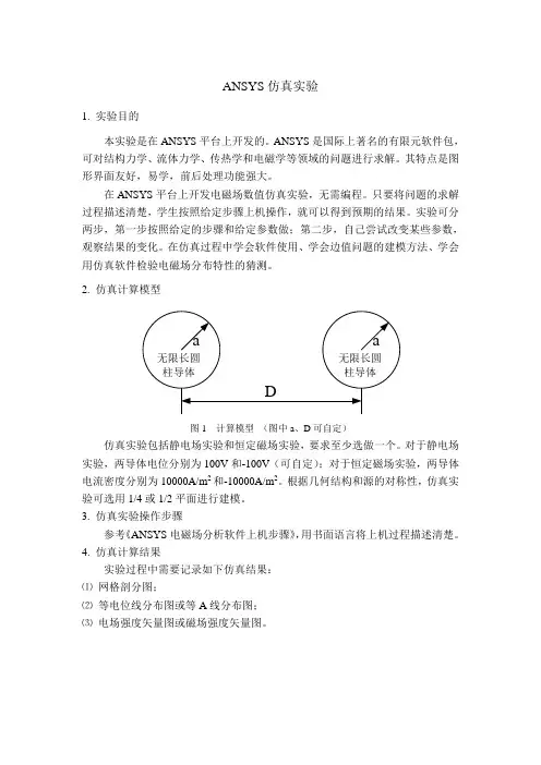
2. 仿真计算模型
图1 计算模型(图中a、D可自定)
仿真实验包括静电场实验和恒定磁场实验,要求至少选做一个。
对于静电场实验,两导体电位分别为100V和-100V(可自定);对于恒定磁场实验,两导体电流密度分别为10000A/m2和-10000A/m2。
根据几何结构和源的对称性,仿真实验可选用1/4或1/2平面进行建模。
3. 仿真实验操作步骤
参考《ANSYS电磁场分析软件上机步骤》,用书面语言将上机过程描述清楚。
4. 仿真计算结果
实验过程中需要记录如下仿真结果:
⑴网格剖分图;
⑵等电位线分布图或等A线分布图;
⑶电场强度矢量图或磁场强度矢量图。


电磁场仿真实验报告求平行输电线周围的电位和电场分布一、报告要求:该生学号尾号为1,建立3条垂直排布的导线。
电位由下到上分别为1V,2V,3V,如下图所示:二、模型说明:静电场计算,求解区域为模型的5倍,截断边界条件。
最下方导线对地高度为10米,导线半径为0.01米,导线之间间距为5米。
(即:H1=10m,H2=15m,H3=20m,U1=1V,U2=2V,U3=3V,R0=0.01m,求解区域为一半圆,题目要求求解区域为模型的5倍,模型尺寸认为是40m,故取半圆半径L=200m。
)如下图所示:三、实验步骤:1、确定文件名,选择研究范围。
点击Utility Menu>File>Change Title,输入你的文件名。
例如“姓名_学号”(ZLM_2012301530051)点击Main Menu>Preferences,选择Electric。
点击Main Menu>Preprocessor>,进入前处理模块(command: /TITLE,ZLM_2012301530051/COM,Preferences for GUI filtering have been set to display:/COM, Electric/PREP7 )2、定义参数点击Utility Menu>Parameters>Scalar Parameters,在下面“Selection”空白区域填入参数:H1=10H2=15H3=20R0=0.01U1=1U2=2U3=3每一个参数输入完毕,点击“Accept ”按钮,输入的参数就导入上方“Items”指示的框中,等参数导入完毕后,点击“close”按钮关闭对话框。
(command: *SET,H1,10*SET,H2,15*SET,H3,20*SET,R0,0.01*SET,U1,1*SET,U2,2*SET,U3,3)3、定义单元类型点击Main Menu>Preprocessor>Element Type>Add/Edit/Delete,出现单元类型对话框“Element Types”,点击Add,弹出单元类型选择库对话框“Library of ElementTpes”选择Electrostatic 和2D Quad 121(二维四边形单元plane121)。
鼠笼异步电动机磁场的有限元分析摘要鼠笼异步电动机具有结构简单、价格低廉、运行可靠、效率较高、维修方便等一系列的优点,在国民经济中得到广泛的应用。
工业、农业、交通运输、国防工程以及日常生活中都大量使用鼠笼异步电动机。
随着大功率电子技术的发展,异步电动机变频调速得到越来越广泛的应用,使得鼠笼异步电动机在一些高性能传动领域也得到使用。
鼠笼异步电动机可靠性高,但由于种种原因,其故障仍时有发生。
由于电动机结构设计不合理,制造时存在缺陷,是造成故障的原因之一。
对电机内部的电磁场进行正确的磁路分析,是电机设计不可或缺的步骤。
利用有限元法对电机内部磁场进行数值分析,可以保证磁路分析的准确性。
本文利用Ansys Maxwell软件,建立了鼠笼式异步电机的物理模型,并结合数学模型和边界条件,完成了对鼠笼式异步电动机的磁场仿真,得到了物理模型剖分图,磁力线和磁通分布图,为电机的进一步设计研究提供了依据。
关键词:Ansys Maxwell;鼠笼式异步电机;有限元分析一、前言当电机运行时,在它的内部空间,包括铜与铁所占的空间区域,存在着电磁场,这个电磁场是由定、转子电流所产生的。
电机中电磁场在不同媒介中的分布、变化及与电流的交链情况,决定了电机的运行状态与性能。
因此,研究电机中的电磁场对分析和设计电机具有重要的意义。
在对应用于交流传动的异步电机进行电磁场的分析计算时,传统的计算方法因建立在磁场简化和实验修正的经验参数的基础之上,其计算精度就往往不能满足要求。
如果从电磁场的理论着手,研究场的分布,再根据课题的要求进行计算,就有可能得到满意的结果。
电机电磁场的计算方法大致可以分为解析法、图解法、模拟法和数值计算法。
数值解法是将所求电磁场的区域剖分成有限多的网格或单元,通过数学上的处理,建立以网格或单元上各节点的求解函数值为未知量的代数方程组。
由于电子计算机的应用日益普遍,所以电机电磁场的数值解法得到了很大发展,它的适用范围超过了所有其它的解法,并能达到足够的精度。

IntroductionThe Magnetic Valve includes a fixed and a rotating part. The rotating body has to move, as quickly as possible, to rest in one of the 2 possible stop positions. Driving current patterns are the input to generate suitable torques. The customer experienced different performances of the valve for different current patterns: sometimes he got strong bumps on the mechanic stops and failures of the valve behaviour. the customer decided to commit a simulation of the magnetic and dynamic behaviour of the valve, instead to build a prototype.Analysis GoalThe goal is ton achieve measure of the Magnetic Torque, as function of current and rotation angle within a parametric approachOwner:EnginsoftUsage Restrictions:Freely available for useIndustry:AutomotiveApplication:ValvePhysics:ElectromagneticsProduct(s)/Version:ANSYS-v10.1Geometry Type(s):SolidGeometry Format(s): Design ModelerModel Size:147070 Nodes, 105742 ElementsElement Type(s): Edge 117Estimated Demo Time:15 Minutes to show, 12 minutes running timeCustomer:Competition:Comsol,AnsoftChallenge:Free accurate Mesh, Parametric Model, Non LinearMagnetic AnalysisKey Features Used:Sphere of influence for meshing, BH Non Linear Curvedata import, Parametric AnalysisSteps and Points to Convey.Picture Guide.Start ANSYS Workbench Environment, and choose “New Geometry”.Importing of external geometrySet the desired length unit: meters.01) Click “File > Open > Import External Geometry File”.02) Click on “Generate” in order to confirm the importation of the geometry.The geometry regards a magnetic valve.Steps and Points to Convey.Picture Guide.Create a Parametric, Relative Rotation between two groups of bodies01) Create a local coordinate system (plane 4) by clicking on the “New Plane” icon in the tool bar.02) In “Details of Plane4 >. Type” choose from face in order to select the surface of interest. 03) Choose the space to the right of “Base Face” in Details of Plane4 and select the surface indicated in light blue in the plot at right.The local coordinate system “Plane 4” is now visible, centered on a face vertex04) In “Details of Plane4 >. Transform 1 (RMB)” insert an offset along X axis of –0.00825 m.05) In “Details of Plane4 >. Transform 1 (RMB)” insert an offset along Y axis of 0.0015 m.06) Click Generate to create Plane4Create another plane (Plane5).07) In “Details of Plane5 > Type” choose from plane. Base plane should be set to Plane4.08) In “Details of Plane5 >. Transform 1 (RMB)” insert a rotation about Z axis of 30°. 09) Click Generate to create Plane5.Steps and Points to Convey. Picture Guide.The local coordinate system “Plane 5” is now visible.10) From the tool bar menu, select “Tools > Freeze”.The freezing operation is indicated when bodies are displayed with transparency.11) From the tool bar menu, select “Create > Body Operation” set “Type” to “Move” click on the box to the right of Bodies.12) Select the bodies highlighted at right (use the Ctrl button to select multiple entities) and click Apply.Steps and Points to Convey.Picture Guide.13) In “Details of BodyOp1” choose the box to the right of “Source Plane” and pick on Plane4 in the Tree Outline.14) In a similar fashion, set “Destination Plane” to Plane5.Then click on “Generate” to move the parts as shown at right.ENCLOSURE definition01) From the tool bar menu, select “Tools >Enclosure” in order to insert a control volume cylindrically shaped and aligned to Y axis. Set the Cushion to 0.0375 m and set “Merge Parts?” to “Yes”.02) Click Generate to create the enclosureIn the “Outline” tree the just created enclosure is now visible.Steps and Points to Convey Picture GuideEnclosure is visible in the “Model View”window.CREATE the WINDING COIL01) In the Tree Outline, Open “1 Part, 7 Bodies > Part”. RMB on the last Solid in the list and choose “Hide Body” in the drop down menu. This will allow access to the surfaces of the imported geometry for forthcoming picking operations.02) Create a new plane (Plane6)03) In “Details of Plane6 >. Type” choose “From Face”.04) Click on the box to the right of “Base Face” and select the surface shown at right.05) In “Details of Plane6 >. Transform 1 (RMB)” insert an offset along Z axis of –0.0231 m.Click on Generate to create Plane6.06) With Plane6 now active, go to the tool bar and choose “New Sketch”.07) Select “Sketch1” in the “Tree Outline”.Steps and Points to Convey Picture Guide Sketching mode for winding coil generation08) Pick the Sketching tab at the bottom of theTree Outline09) Select “Circle” in the “Draw” window andchoose the center (origin of Plane6) and anarbitrary poin some distance away from thecenter to create a circle.10) Pick the Dimensions button at the bottom ofthe Sketching Toolboxes pane and choose“Radius”.11) Click on the circle and another arbitrarylocation for the radial dimension marker.12) In “Details of Sketch1”, modify the radiusR1 to be 0.00775 m.The sketch is now visible in the “Graphics”window.13) From the tool bar select “Concept > LineFrom Sketches”. Choose the circle and clickApply in the box to the right of “Base Objects”in “Details of Line1”. “Operation” should be setto “Add Material”.Click Generate.14) Choose the Line Body in the Tree Outline.15) In “Details of Line Body” set:•“Winding Body > Yes”•“Number of Turns” = 1•“CS Length” = 0.022 m•“CS Length” = 0.00375 mSteps and Points to ConveyPicture Guide16) From the tool bar, select “View > Show Cross Sections Solids”. The new winding body should appear as it does in the figure to the right.ANGLE as PARAMETER01) In the “Tree Outline” select “Plane5”02) Make the rotation about Z axis as parameter by clicking on the box to the left of “FD1, Value 1”.03) Rename the parameter as “angle”.Steps and Points to Convey.Picture Guide.04) From the tool bar, select “Tools > Options>Common Settings>Geometry Import”. Remove “DS” from the field to the right of “Personal Parameter Key” to remove the DS prefix naming convention restriction for importing parameters. Click OK.GO IN SIMULATIONIn the “[Project]” window, select “New Simulation”.In the “[Simulation]” window, the “Outline” tree should be as in figure.Steps and Points to ConveyPicture GuideMaterials Properties DefinitionSelect “Data” in the tool bar to open the “[Engineering Data]” window.Materials Properties Definitionchange defaults of STRUCTURAL STEEL01) Select “Structural Steel” and click on “Add/Remove Properties” in the “Electromagnetics” field and unselect the following items:- “Relative Permeability” - “Resistivity”02) Check the box to the left of “B-H curve” and click OK.03) Say “Yes” to the “Remove Material Properties” box that appears.04) Open excel file “bh1.xls” and copy the two data columns (highlight them with the mouse cursor and type Cntl-C).Steps and Points to ConveyPicture Guide05) Click the icon depicting an xy plot to the right of “B-H Curve”06) LMB on the 2 (second row) of the “Magnetic Flux Density vs. Magnetic Field Intensity” table and press “Ctrl +V” to paste the two column data from the .xls file.07) Click on the B-H Curve icon at the lower right.The curve should appear as shown at right.NEW Material definition IRONRMB on “Materials (2)” in the tree and choose “Insert New Material”. RMB on “New Material”, choose Rename and change the name of the new material to Iron. Define BH data as before but this time use data from “bh2.xls” file.NEW Material definition NEODYMIUM01) Define a New material named “Neodymium”.02) Among Electromagnetics properties let active just: “Linear Hard Material”: 03) Insert the following data:• Cohercive Force: 7.9577 e5 A/m • Residual Induction 1.2 T01) Return to the Simulation Tab02) In the Outline Tree, open Geometry>Part and use the Cntl button to select both of the RIC9512_105 items. The parts should be highlighted as shown at right.03) In Details of “Multiple Selection”, changematerial from “Structural Steel” to “Iron”Steps and Points to ConveyPicture Guide04) Select the part shown at right.05) Change material from “Structural Steel” to “Neodymium”MESH01) Select the coil support solid (see figure)02) RMB on “Mesh” on the tree to insert a sizing control: Element Size 2e-303) Insert another sizing control , 1e-3, referred to 5 bodies as in the following picture. It may help to hide the 4th solid (the “air enclosure) in the Outline tree to simplify selecting these parts.Steps and Points to ConveyPicture Guide5 bodies for sizing setting n.204) In the Outline tree, RMB on Model and insert a “Coordinate Systems” branch. RMB on the Coordinate Systems branch and insert (define) a new Coordinate System. Choose “Origin” in the Details of “Coordinate System” pane, select the surface shown at right, and click Apply.05) RMB on Mesh in the Outline to insert a third sizing control:For “Type”, choose “Sphere of Influence”• Sphere Center: Coordinate System (defined just before) • Radius 1.5e-2 • Element size 5e-4Areas to be applied are the following (10 areas)Steps and Points to ConveyPicture Guide10 Areas where to apply the Sphere of Influence sizing control06) Click on Mesh -> Preview MeshThe Mesh should result as in figure, if the “Air” solid enclosure body is hideLOADSSet the Conductor Current value in details window related to “Conductor Winding Body”: 1000 ABOUNDARY CONDITIONSRMB on Environment in the tree and insert a Magnetic Flux Parallel object. Use the Cntl button to select the 3 exterior surfaces of the enclosure and click Apply.Steps and Points to Convey.Picture Guide.POSTPROCESSING SETTINGS01) Insert under the “Solution” tree the following output requests: • Total Flux Density • Total Flux Intensity 02) Select 3 bodies as in figure03) Insert a “Directional Force/Torque” output request with details:• In Details of “Directional Force/Torque” pane, change “Global Coordinate System” to “Coordinate System” (this is the user-defined coordinate system centered on the top surface of the permanent magnet).• Set Orientation to Y Direction (rotation axis)04) repeat Directional Force/Torque Request for both X and Z axis direction05) By a right click under the Solution Tree Insert a “Solution Information” request to monitor the run during the solutionSOLVE01) Highlight the Environment tree tosee/check all Boundary & Loads previously defined.02) Click on the “SOLVE” Icon to launchthe run.Solution times takes about 12 minutes on a 2.8 Ghz single processor 32bit PCSteps and Points to ConveyPicture GuideREVIEW RESULTS01) See the Total Flux of Magnetic results 02) Set up a Vector Image of the MagneticField03) After Vector Image settings show a Vector Plot of Magnetic Field03)See the Magnetic Force distribution, Yaxis direction, on the requested parts. 04)The same for X, Z directions05)Activate the view from Y Global Axis06)Define a “Slice Plane”07)Draw the slice plane trace at nearlyalong the Y global direction08)View from the X Global direction09)Activate “show elements” and show themagnetic fieldSteps and Points to Convey Picture GuideSET UP A PARAMETRIC ANALYSIS01) Click on “Model”02) Click on CAD Parameters Detail toactivate the “angle” as a parameter. Thiswill be the first INPUT parameter.03) Click on Environment and Duplicate byright click04) Activate the Conductor Current Value asparameter. This is the second INPUTparameter n.2.05) Activate the Torque value in Y directionas OUTPUT parameter (ThirdParameter)06)Click on “Solution” of Environment 2and then click on Parameter Manager 07)Set up many cases as you like, forexample with 4 current values, 3 values other than the previously solved.。