用Design-Expert软件进行响应曲面分析
- 格式:pptx
- 大小:1.80 MB
- 文档页数:23
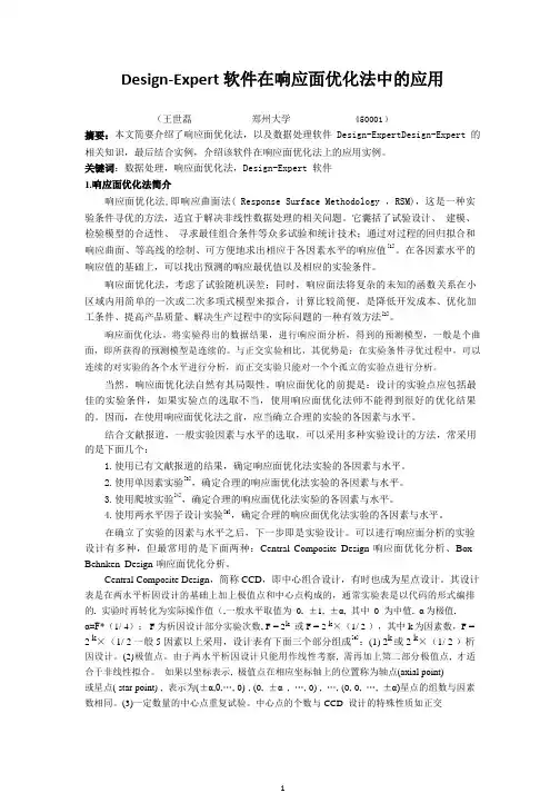
Design-Expert 软件在响应面优化法中的应用(王世磊郑州大学450001)摘要:本文简要介绍了响应面优化法,以及数据处理软件Design-ExpertDesign-Expert的相关知识,最后结合实例,介绍该软件在响应面优化法上的应用实例。
关键词:数据处理,响应面优化法,Design-Expert软件1.响应面优化法简介响应面优化法,即响应曲面法( Response Surface Methodology ,RSM),这是一种实验条件寻优的方法,适宜于解决非线性数据处理的相关问题。
它囊括了试验设计、建模、检验模型的合适性、寻求最佳组合条件等众多试验和统计技术;通过对过程的回归拟合和响应曲面、等高线的绘制、可方便地求出相应于各因素水平的响应值[1]。
在各因素水平的响应值的基础上,可以找出预测的响应最优值以及相应的实验条件。
响应面优化法,考虑了试验随机误差;同时,响应面法将复杂的未知的函数关系在小区域内用简单的一次或二次多项式模型来拟合,计算比较简便,是降低开发成本、优化加工条件、提高产品质量、解决生产过程中的实际问题的一种有效方法[2]。
响应面优化法,将实验得出的数据结果,进行响应面分析,得到的预测模型,一般是个曲面,即所获得的预测模型是连续的。
与正交实验相比,其优势是:在实验条件寻优过程中,可以连续的对实验的各个水平进行分析,而正交实验只能对一个个孤立的实验点进行分析。
当然,响应面优化法自然有其局限性。
响应面优化的前提是:设计的实验点应包括最佳的实验条件,如果实验点的选取不当,使用响应面优化法师不能得到很好的优化结果的。
因而,在使用响应面优化法之前,应当确立合理的实验的各因素与水平。
结合文献报道,一般实验因素与水平的选取,可以采用多种实验设计的方法,常采用的是下面几个:1.使用已有文献报道的结果,确定响应面优化法实验的各因素与水平。
2.使用单因素实验[3],确定合理的响应面优化法实验的各因素与水平。


第一步,打开Design-Expert软件第二步,新建一个设计(File----New Design)画面变成下图:第三步,在左侧点击Response Surface,变成下图:一般响应面中Central Composite是5水平,而Box-Behnken是3水平,所以选Box-Behnken,即单击左侧的Box-Behnken设计方法,变成下图:第四步,由于是三因素三水平,所以在Numeric Factors 这一栏选择“3”,表示3因素,并在下表中改好名字,填好单位;把-1水平和+1水平分别填上。
如皂土用量-1为2.5mL,+1为4.5mL。
如下图:注:其他所有选项都不需要改。
第五步,点击右下角“continue”键,进入下一页面:这里是响应值,对应本次实验里的透光率,把名字改好,单位填上,如图:第六步,点击“continue”键,进入实验设计表格:根据具体的实验条件将实验值一个一个地填上(实验值也就是从对应的实验条件下获得的真实数据),得到第七步,对数据进行分析。
对我们有用的是左侧的“Analysis”项,点击它,得到:可以先大致看一下,然后点响应值“透光率”,也就是“Analysis”的子菜单。
得到图:不管,点击第二个“summary”,得到:这里有一些数据模型的基本信息,基本上不怎么用得到,可以看一下。
然后继续点击“Model”,得到:基本上也不用管,继续点击“ANOV A”,得到:这里才有我们需要的东西,比如显著性,数学模型等等,很多论文中的表格、方差分析都是从这里来的,这一项很有用,可以慢慢看。
然后再继续,点击“Diagnostics”,这里基本上是关于数据分散性的,用处不大。
有3D图和等高线图的地方。
如图:如果点击“Model Graphs”没有出现3D图,可以点击菜单栏的view,找出“3D Surface”,点击,就可以出来了。
同理,要想出等高线图,可以在菜单栏的view中找出“Contour”,点击即可,即:以上是响应面的基本信息及基本出图,下面是如何用响应面做最优条件的选择。
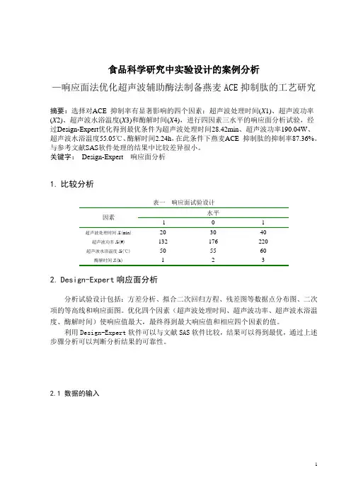
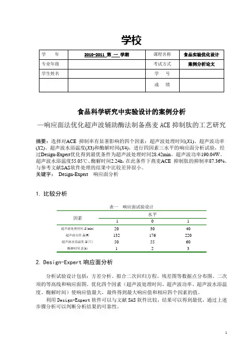
食品科学研究中实验设计的案例分析—响应面法优化超声波辅助酶法制备燕麦ACE抑制肽的工艺研究摘要:选择对ACE 抑制率有显著影响的四个因素:超声波处理时间(X1)、超声波功率(X2)、超声波水浴温度(X3)和酶解时间(X4),进行四因素三水平的响应面分析试验,经过Design-Expert优化得到最优条件为超声波处理时间28.42min、超声波功率190.04W、超声波水浴温度55.05℃、酶解时间2.24h,在此条件下燕麦ACE 抑制肽的抑制率87.36%。
与参考文献SAS软件处理的结果中比较差异很小。
关键字: Design-Expert 响应面分析1.比较分析表一响应面试验设计水平因素-1 0 1 超声波处理时间X1(min) 20 30 40超声波功率X2(W) 132 176 220超声波水浴温度X3(℃) 50 55 60 酶解时间X4(h) 1 2 3 2.Design-Expert响应面分析分析试验设计包括:方差分析、拟合二次回归方程、残差图等数据点分布图、二次项的等高线和响应面图。
优化四个因素(超声波处理时间、超声波功率、超声波水浴温度、酶解时间)使响应值最大,最终得到最大响应值和相应四个因素的值。
利用Design-Expert软件可以与文献SAS软件比较,结果可以得到最优,通过上述步骤分析可以判断分析结果的可靠性。
2.1 数据的输入图 1 2.2 Box-Behnken响应面试验设计与结果图 2 2.3 选择模型图 32.4 方差分析图 4在本例中,模型显著性检验p<0.05,表明该模型具有统计学意义。
由图4知其自变量一次项A,B,D,二次项AC,A2,B2,C2,D2显著(p<0.05)。
失拟项用来表示所用模型与实验拟合的程度,即二者差异的程度。
本例P值为0.0861>0.05,对模型是有利的,无失拟因素存在,因此可用该回归方程代替试验真实点对实验结果进行分析。
第一步,打开Design-Expert软件第二步,新建一个设计(File----New Design) 画面变成下图:一般响应面中 Central Composite 是 5水平,而Box-Behnken 是 3 水平,所以选 Box-Behnken ,即单击左侧的Box-Behnken 设计方法,变成下图:2-Level Factorial EtesignC^sign-tai StaJI U:twi 皆w 4Kh factaiii-miM cm* 1L^tful br45t«nalrig mah 4IKI5 ind iNerKlMM: Fr-artE^al Pirfc! cati tn uMdio* 乂rqtn nj mam Actors l»4id tie - sqiilcifv:^- Fw catarkEilf^ w 创塔细E BA tHtiibTi iMNuUrl Of A th ■ PAE V4i liprA■- YMbw-Rtid W, Arid RUS- R 鮭 11用BIF 關Tl MiflAiilR«AV Mm 口 KI R I罕 M EjdarFrwtkin 也閒id |>QP|rnalPiwHrtBjimah TftawhiMM Ld M LA bu■J■13M1& liSr?143t4212T■23 K'IS2"n 乩丫 * IV? ■■老5-1空0-] 10-511-5 J勺 I2-? rh ITS 、1M 二 w勺 15-10 即-M26* M雷少 10-4 忆M ? n-s 止IV乡 li-fi 丁 E* un M-kl* wA 1S-# 忆¥n- itiQ * rv ? IT-11£即E 酣 l A-13 * IVrj M-H 忆¥2?•y B-l £皿2:12T勢£和n 1]■& W r/1 47Jn 15-* ■=-hrT 149 匚M 予“IDn 19-11W & 亍IfrU丄 n JO 13 丄N ZLE-2・2;1 n 1Q-T * H 7 H-3 疋VI2'-- 空¥| n. I A3* V 幷,M-B E M* n 计€ V 7 It-D2;Mn ia-in * M右' 9 n-ii11T2° n 16iW K 211-1匚71n- 11-4 Jn 15 t€ MQ 1 i-T直VI7 17-3 £ ¥1n T*E> 铲2™11B^s I ・C AHMCulnut ・A第三步,在左侧点击 Response Surface 变成下图:E* Sjfctflel JI- _J2JSLjrfiiij piitirrH-n»>j4r1 屈 iarttAidd Mu 畤嘔 |J* CZIaH^.e-ir-si to丸『:电rm Central Composite Design Eich rwn^c I FM K: N 诸 and rrism □tsM I >MI coris^, pLs irri moji 1 祗血” p(#!hi arxi he [tfTW pom f cairgco: Rirkus ire vlv^i, he- rentni conpasrki di^pi w*«&ckiE ■:旳xl ftc Mff ciWnStrtMlin tfHA iMia J H" 1 s ・ 1 -ME 1科“ 11 '叫1 Xp 1"I 1j 彳 .1 11 亦 |l iT ■”■ Er*■- iiOQ r«igKLin Irru -il 亦 lkw«taErfcr iKwr4ngM.« ■R [hf 6WWC •FvHcRHICMttfpOilS 8CwsrpeHi f13加 W COrililUG- ■>第四步,由于是三因素三水平,所以在Numeric Factors 这一栏选择“3”,表示3因素,并在下表中改好名字,填好单位;把-1水平和+1水平分别填上。
DX7-04C-MultifactorRSM-P1.doc Rev. 4/12/06Multifactor RSM Tutorial (Part 1 – The Basics)Response Surface Design and AnalysisThis tutorial shows the use of Design-Expert® software for response surface methodology (RSM). This class of designs is aimed at process optimization. A case study provides a real-life feel to the exercise. Due to the specific nature of the case study, a number of features that could be helpful to you for RSM will not be exercised in this tutorial. Many of these features are used in the General One Factor, RSM One Factor or Two-Level Factorial tutorials. If you have not completed all of these tutorials, consider doing so before starting in on this one. We will presume that you can handle the statistical aspects of RSM. For a good primer on the subject, see RSM Simplified (Anderson and Whitcomb, Productivity, Inc., New York). You will find overviews on RSM and how it’s done via Design-Expert in the online Help system. To gain a working knowledge of RSM, we recommend you attend our Response Surface Methods for Process Optimization workshop. Call Stat-Ease or visit our website, , for a schedule. The case study in this tutorial involves production of a chemical. The two most important responses, designated by the letter “y”, are: • • y1 - Conversion (% of reactants converted to product) y2 - Activity.The experimenter chose three process factors to study. Their names and levels can be seen in the following table.FactorA – Time B - Temperature C - CatalystUnitsminutes degrees C percentLow Level (-1)40 80 2High Level (+1)50 90 3Factors for response surface study You will study the chemical process with a standard RSM design called a central composite design (CCD). It’s well suited for fitting a quadratic surface, which usually works well for process optimization. The three-factor layout for the CCD is pictured below. It is composed of a core factorial that forms a cube with sides that are two coded units in length (from -1 to +1 as noted in the table above). The stars represent axial points. How far out from the cube these should go is a matter for much discussion between statisticians? They designate this distance “alpha” – measured in terms of coded factor levels. As you will see Design-Expert offers a variety of options for alpha.Design-Expert 7 User’s GuideMultifactor RSM Tutorial – Part 1 • 1Central Composite Design for three factors Assume that the experiments will be conducted over a two-day period, in two blocks: 1. Twelve runs: composed of eight factorial points, plus four center points. 2. Eight runs: composed of six axial (star) points, plus two more center points.Design the ExperimentStart the program by finding and double clicking the Design-Expert software icon. Take the quickest route to initiating a new design by clicking the blank-sheet icon on the left of the toolbar. The other route is via File, New Design (or associated Alt keys).Main menu and tool bar Click on the Response Surface folder tab to show the designs available for RSM.Response surface design tab The default selection is the Central Composite design, which will be used for this case study. Click on the down arrow in the Numeric Factors entry box and Select 3. Ignore the option of including categoric factors in your designs (leave at default of 0).2 • Multifactor RSM Tutorial – Part 1Design-Expert 7 User’s GuideDX7-04C-MultifactorRSM-P1.doc Rev. 4/12/06To see alternative RSM designs for three factors, click on the choices for BoxBehnken (17 runs) and Miscellaneous designs, where you find the 3-Level Factorial option (32 runs, including 5 center points). Now go back and re-select the Central Composite design. Before entering the factors and ranges, click the Options at the bottom of the CCD screen. Notice that it defaults to a Rotatable design with the axial (star) points set at 1.68719 coded units from the center – a conventional choice for the CCD. For Center points increase the number to the normal default of 6 and press the Tab key.Default CCD option for alpha set so design will be rotatable Many of the options are statistical in nature, but one that produces less extreme factor ranges is the “Practical” value for alpha. This is computed by taking the fourth root of the number of factors (in this case 3¼ or 1.31607). See RSM Simplified Chapter 8 “Everything You Should Know About CCDs (but dare not ask!)” for details on this practical versus other levels suggested for alpha in CCDs – the most popular of which may be the “Face Centered” (alpha equal one). Press OK to accept the rotatable value. Using the information provided in the table on page 1 of this tutorial (or on the screen capture below), type in the details for factor Name (A, B, C), Units and levels for low (-1) and high (+1), by tabbing or clicking to each cell and entering the details given in the introduction to this case study.Completed factor formDesign-Expert 7 User’s GuideMultifactor RSM Tutorial – Part 1 • 3You’ve now specified the cubical portion of the CCD. As you did this, Design-Expert calculated the coded distance “alpha” for placement on the star points in the central composite design. Alternatively, by clicking an option further down this screen, you could have entered values for alpha levels and let the software figure out the rest. This would be helpful if you wanted to avoid going out of operating constraints. Now go back to the bottom of the central composite design form. Leave the Type at its default value of Full (the other option is a “small” CCD, which we do not recommend unless you must cut the number of runs to the bare minimum). You will need two blocks for this design, one for each day, so click on the Blocks field and select 2.Selecting the number of blocks Notice that the software displays how this CCD will be laid out in the two blocks. Click on the Continue button to reach the second page of the “wizard” for building a response surface design. You now have the option of identifying Block Names. Enter Day 1 and Day 2 as shown below.Block names Press Continue to enter Responses. Select 2 from the pull down list. Then enter the response Name and Units for each response as shown below.Completed response form At any time in the design-building phase, you can return to the previous page by pressing the Back button. Then you can revise your selections. Press the Continue button to get the design layout (your run order may differ due to randomization).4 • Multifactor RSM Tutorial – Part 1Design-Expert 7 User’s GuideDX7-04C-MultifactorRSM-P1.doc Rev. 4/12/06Design layout (only partially shown, your run order may differ due to randomization) Design-Expert offers many ways to modify the design and how it’s laid out on-screen. Preceding tutorials, especially in Part 2 for the General One Factor, delved into this in detail, so go back and look this over if you haven’t already. Click the Tips button for a refresher.Save the Data to a FileNow that you’ve invested some time into your design, it would be prudent to save your work. Click on the File menu item and select Save As.Save As selection You can then specify the File name (we suggest tut-RSM) to Save as type *.dx7” in the Data folder for Design-Expert (or wherever you want to Save in).Design-Expert 7 User’s GuideMultifactor RSM Tutorial – Part 1 • 5File Save As dialog boxEnter the Response Data – Create Simple Scatter PlotsAssume that the experiment is now completed. Obviously at this stage the responses must be entered into Design-Expert. We see no benefit to making you type all the numbers, particularly with the potential confusion due to differences in randomized run orders. Use the File, Open Design menu and select RSM.dx7 from the Design-Expert program Data directory. Click on Open to load the data. Let’s examine the data, which came in with the file you opened (no need to type it in!). Move your cursor to the top of the Std column and perform a right-click to bring up a menu from which you should select Sort by Standard Order (this could also be done via the View menu).Sorting by Standard (Std) Order Next go to the Block column and do a right click. Choose Display Point Type.6 • Multifactor RSM Tutorial – Part 1Design-Expert 7 User’s GuideDX7-04C-MultifactorRSM-P1.doc Rev. 4/12/06Displaying the Point Type (Notice that we widened the column so that you can see how some points are labeled “Fact” for factorial and others “Center” for center point, etc. Do this by placing your mouse cursor over the border and, when it changes to a double-arrow [↔], drag it where you want. Some times this does not work the first time, but do not be discouraged: It will probably work the second time. What a drag!) Before doing the analysis, it might be interesting to take a look at some simple plots. Click on the Graph Columns node which branches from the design ‘root’ at the upper left of your screen. You should now see a scatter plot with factor A:Time on the X-axis is set at and the response of Conversion on the Y-axis. It will be much more productive to see the impact of the control factors on response surface graphics to be produced later. For now it would be most useful to produce a plot showing the impact of blocks, because this will be literally blocked out in the analysis. On the floating Graph Columns tool click on the X Axis downlist symbol and select Block.Design-Expert 7 User’s GuideMultifactor RSM Tutorial – Part 1 • 7Graph Columns feature for design layout The graph shows a slight correlation (0.152) of conversion by block. Change the Y Axis to Activity to see how it’s affected by the day-to-day blocking (not much!).Changing response (resulting graph not shown) Finally, to see how the responses correlate with each other, change the X Axis to Conversion.Plotting one response versus the other (resulting graph not shown) Feel free to make other scatter plots. Notice that you can also color the by selected factors, including run (the default). However, do not get carried away with this, because it will be much more productive to do statistical analysis first before drawing any conclusions.8 • Multifactor RSM Tutorial – Part 1Design-Expert 7 User’s GuideDX7-04C-MultifactorRSM-P1.doc Rev. 4/12/06Analyze the ResultsYou will now start analyzing the responses numerically. Under the Analysis branch click the node labeled Conversion. A new set of buttons appears at the top of your screen. They are arranged from left to right in the order needed to complete the analysis. What could be simpler?Begin analysis of Conversion Design-Expert provides a full array of response transformations via the Transform option. Click Tips for details. For now, accept the default transformation selection of None. Click on the Fit Summary button next. At this point Design-Expert fits linear, twofactor interaction (2FI), quadratic and cubic polynomials to the response. To move around the display, use the side and/or bottom scroll bars. You will first see the identification of the response, immediately followed in this case by a warning: “The Cubic Model is Aliased.” Do not be alarmed. By design, the central composite matrix provides too few unique design points to determine all of the terms in the cubic model. It’s set up only for the quadratic model (or some subset). Next you will see several extremely useful summary tables for model selection. Each of these tables will be discussed briefly below. The table of “Sequential Model Sum of Squares” (technically “Type I”) shows how terms of increasing complexity contribute to the total model. The model hierarchy is described below: • • “Linear vs Block”: the significance of adding the linear terms to the mean and blocks, “2FI vs Linear”: the significance of adding the two factor interaction terms to the mean, block and linear terms already in the model,Design-Expert 7 User’s GuideMultifactor RSM Tutorial – Part 1 • 9•“Quadratic vs 2FI”: the significance of adding the quadratic (squared) terms to the mean, block, linear and two factor interaction terms already in the model, “Cubic vs Quadratic”: the significance of the cubic terms beyond all other terms.•Sequential Model Sum of Squares For each source of terms (linear, etc.), examine the probability (“Prob > F”) to see if it falls below 0.05 (or whatever statistical significance level you choose). So far, the quadratic model looks best – these terms are significant, but adding the cubic order terms will not significantly improve the fit. (Even if they were significant, the cubic terms would be aliased, so they wouldn’t be useful for modeling purposes.) Scroll down to the next table for lack of fit tests on the various model orders.Summary Table: Lack of Fit Tests The “Lack of Fit Tests” table compares the residual error to the “Pure Error” from replicated design points. If there is significant lack of fit, as shown by a low probability value (“Prob>F”), then be careful about using the model as a response predictor. In this10 • Multifactor RSM Tutorial – Part 1Design-Expert 7 User’s GuideDX7-04C-MultifactorRSM-P1.doc Rev. 4/12/06case, the linear model definitely can be ruled out, because its Prob > F falls below 0.05. The quadratic model, identified earlier as the likely model, does not show significant lack of fit. Remember that the cubic model is aliased, so it should not be chosen. Scroll down to the last table in the Fit Summary report, which provides “Model Summary Statistics” for the ‘bottom line’ on comparing the options.Summary Table: Model Summary Statistics The quadratic model comes out best: It exhibits low standard deviation (“Std. Dev.”), high “R-Squared” values and a low “PRESS.” The program automatically underlines at least one “Suggested” model. Always confirm this suggestion by looking at these tables. Check Tips for more information about the procedure for choosing model(s). Design-Expert now allows you to select a model for an in-depth statistical study. Click on the Model button at the top of the screen next to see the terms in the model.Model resultsDesign-Expert 7 User’s GuideMultifactor RSM Tutorial – Part 1 • 11The program defaults to the “Suggested” model from the Fit Summary screen. If you want, you can choose an alternate model from the Process Order pull-down list. (Be sure to do this in the rare cases when Design-Expert suggests more than one model.)The options for process order At this stage you could press the Add Term button and insert higher degree terms with integer powers, such as quartic (4th degree). However, for this case study, we’ll leave the selection at Quadratic. You could now manually reduce the model by clicking off insignificant effects. For example, you will see in a moment that several terms in this case are marginally significant at best. Design-Expert also provides several automatic reduction algorithms as alternatives to the “Manual” method: “Backward,” “Forward” and “Stepwise.” Click the down arrow on the Selection list box to use these. Click on the ANOVA button to produce the analysis of variance for the selected model. The ANOVA table is available in two views. By default it will add text providing brief explanations and guidelines to the reported statistics. To turn this off, choose View, Annotated ANOVA. Notice that this toggles off the check mark (√).Statistics for selected model: ANOVA table12 • Multifactor RSM Tutorial – Part 1Design-Expert 7 User’s GuideDX7-04C-MultifactorRSM-P1.doc Rev. 4/12/06The ANOVA in this case confirms the adequacy of the quadratic model (the Model Prob>F is less than 0.05.) You can also see probability values for each individual term in the model. You may want to consider removing terms with probability values greater than 0.10. Use process knowledge to guide your decisions. Next, see that Design-Expert presents various statistics to augment the ANOVA – most notably various R-Squared values. These look very good.Post-ANOVA statistics Scroll down to bring the following details on model coefficients to your screen. The mean effect shift for each block is listed here too. (Under certain circumstances the display may be adversely affected when scrolled. To rectify this problem, maximize the screen by clicking the icon at upper right of Windows.)Coefficients for the quadratic model Again scroll down to bring the next section to your screen: the predictive models in terms of coded versus actual factors (shown side-by-side below). Block terms are left out. These terms can be used to re-create the results of this experiment, but they cannot be used for modeling future responses.Design-Expert 7 User’s GuideMultifactor RSM Tutorial – Part 1 • 13Final equation: coded versus actual You cannot edit any of the ANOVA outputs. However, you can copy and paste the data to your favorite Windows word processor or spreadsheet.Diagnose the Statistical Properties of the ModelThe diagnostic details provided by Design-Expert can best be digested by viewing plots the come with a click on the Diagnostics button. The most important diagnostic, the normal probability plot of the residuals, comes up by default.Normal probability plot of the residuals14 • Multifactor RSM Tutorial – Part 1Design-Expert 7 User’s GuideDX7-04C-MultifactorRSM-P1.doc Rev. 4/12/06The data points should be approximately linear. A non-linear pattern (look for an Sshaped curve) indicates non-normality in the error term, which may be corrected by a transformation. There are no signs of any problems in our data. At the left of the screen you see the Diagnostics Tool palette. First of all, notice that residuals will be studentized unless you uncheck the first box on the floating tool palette (not advised). This counteracts varying leverages due to location of design points. For example, the center points carry little weight in the fit and thus exhibit low leverage. Each button on the palette represents a different diagnostics graph. Check out the other graphs if you like. Explanations for most of these graphs were covered in prior Tutorials. In this case, none of the graphs indicate any cause for alarm. Now click the option for Influence. Here’s where you find the find plots for externally studentized residuals (better known as “outlier t”) and other plots that may be helpful for finding problem points in the design. Also, from here you can click Report to bring up a detailed case-by-case diagnostic statistics, many of which have already been shown graphically. (In previous versions of Design-Expert, this report appeared under ANOVA.)Diagnostics report The note below the table (“Predicted values include block corrections.”) alerts you that any shift from block 1 to block 2 will be included for purposes of residual diagnostics. (Recall that block corrections did not appear in the predictive equations shown in the ANOVA report.) Also note that one value of DFFITS is flagged. As we discussed in the General One-Factor Tutorial (Part 2 – Advanced Features), this statistic stands for difference in fits. It measures the change in each predicted value that occurs when that response is deleted. To see what program Help says about DFFFITs, right-click the number.Design-Expert 7 User’s GuideMultifactor RSM Tutorial – Part 1 • 15Accessing context-sensitive Help Given that only this one diagnostic is flagged, it probably is not a cause for alarm. Press X to close out the screen tip provided by the program’s Help system.Examine Model GraphsThe diagnosis of residuals reveals no statistical problems, so you will now generate the response surface plots. Click on the Model Graphs button. The 2D contour plot of factors A versus B comes up by default in graduated color shading.Response surface contour plot Note that Design-Expert will display any actual point included in the design space shown. In this case you see a plot of conversion as a function of time and temperature at a mid-level slice of catalyst. This slice includes six center points as indicated by the dot at the middle of the contour plot. By replicating center points, you get a very good power of prediction at the middle of your experimental region. The Factors Tool comes along with the default plot. Move this floating tool as needed by clicking on the top blue border and dragging it. The tool controls which factor(s) are16 • Multifactor RSM Tutorial – Part 1Design-Expert 7 User’s GuideDX7-04C-MultifactorRSM-P1.doc Rev. 4/12/06plotted on the graph. The Gauges view is the default. Each factor listed will either have an axis label, indicating that it is currently shown on the graph, or a red slider bar, which allows you to choose specific settings for the factors that are not currently plotted. The red slider bars will default to the midpoint levels of the factors not currently assigned to axes. You can change a factor level by dragging the red slider bars or by right clicking on a factor name to make it active (it becomes highlighted) and then typing the desired level in the numeric space near the bottom of the tool palette. Click on the C:Catalyst toolbar to see its value. Don’t worry if it shifts a bit – we will instruct you on how to reset it in a moment.Factors tool with factor C highlighted and value displayed Click down on the red bar with your mouse and push it to the right.Slide bar for C pushed right to higher value As indicated by the color key on the left, the surface becomes ‘hot’ at higher response levels, yellow in the ’80’s and red above 90 for conversion. To enable a handy tool for reading coordinates off contour plots, go to View, Show Crosshairs Window.Design-Expert 7 User’s GuideMultifactor RSM Tutorial – Part 1 • 17Showing crosshairs window Now move your mouse over the contour plot and notice that Design-Expert generates the predicted response for specific values of the factors that correspond to that point. If you place the crosshair over an actual point, for example – the one at the upper left corner of the graph now on screen, you also get that observed value (in this case: 66).Prediction at coordinates of 40 and 90 where an actual run was performed Now press the Default button to put factor C back at its midpoint. Then switch to the Sheet View by clicking on the Sheet button.Factors tool – Sheet view18 • Multifactor RSM Tutorial – Part 1Design-Expert 7 User’s GuideDX7-04C-MultifactorRSM-P1.doc Rev. 4/12/06In the columns labeled Axis and Value you can change the axes settings or type in specific values for factors. Return to the default view by clicking on the Gauges button. At the bottom of the Factors Tool is a pull-down list from which you can also select the factors to plot. Only the terms that are in the model are included in this list. If you select a single factor (such as A) the graph will change to a One Factor Plot. From this view, if you now choose a two-factor interaction term (such as AC) the plot will become the interaction graph of that pair. The only way to get back to a contour graph is to use the menu item View, Contour.Perturbation PlotWouldn’t it be handy to see all your factors on one response plot? You can do this with the perturbation plot, which provides silhouette views of the response surface. The real benefit from this plot is for selecting axes and constants in contour and 3D plots. Use the View, Perturbation menu item to select it.The Perturbation plot with factor A clicked to highlight it For response surface designs the perturbation plot shows how the response changes as each factor moves from the chosen reference point, with all other factors held constant at the reference value. Design-Expert sets the reference point default at the middle of the design space (the coded zero level of each factor). Click on the curve for factor A to see it better. (The software will highlight it with a different color.) In this case, you can see that factor A (time) produces a relatively small effect as it changes from the reference point. Therefore, because you can only plot contours for two factors at a time, it makes sense to choose B and C, and slice on A.Design-Expert 7 User’s GuideMultifactor RSM Tutorial – Part 1 • 19Contour Plot: RevisitedLet’s look at the contour plot of factors B and C. Return to the contour plots via the View, Contour selection.Back to Contour view In the Factors Tool right click on the Catalyst bar palette. Then select X1 axis by left clicking on it.Making factor C the x1-axis You now see a catalyst versus temperature plot of conversion, with time held as a constant at its midpoint. The colors are neat, but what if you must print the graphs in black and white? That can be easily fixed by right-clicking over the graph and selecting Graph Preferences.Graph preferences Click the Graphs 2 tab and change the Contour graph shading to Std Error shading.20 • Multifactor RSM Tutorial – Part 1Design-Expert 7 User’s GuideDX7-04C-MultifactorRSM-P1.doc Rev. 4/12/06Changing contour graph shading Press OK to see the effect on your plot. Change factor A:time by dragging the slider left. See how it affects the shape of the contours. Also, notice how the plot darkens as you approach the extreme. You’re getting into areas of extrapolation. Be careful out there!Contour plot with standard error shading (shows up when A set at lowest level) Put the slider back at its center point by pressing the Default button. As you’ve no doubt observed by now, Design-Expert contour plots are highly interactive. For example, move your mouse over the center point. Notice that it turns into a crosshair ( ) and the prediction appears in the Crosshairs Window along with the X1-X2 coordinate. (If you do not see crosshairs, go to View, Show Crosshairs Window.) For more statistical detail, such as the very useful individual prediction interval (PI), can be found by pressing the Full button.Design-Expert 7 User’s GuideMultifactor RSM Tutorial – Part 1 • 21Crosshairs Window set to Full display of statistics Watch what happens to the numbers as you mouse the cross-hairs around the plot. We hope you are sitting down because it may make you dizzy! Perhaps it may be best if you press the Small button before passing out and falling on to the floor. Design-Expert draws five contour levels by default. They range from the minimum response to the maximum response. Click on a contour to highlight it. You can move the contours by dragging them to new values. (Place the mouse cursor on the contour and hold down the left button while moving the mouse.) Give this a try – it’s fun! Also you can add new contours via a right mouse click. Find a vacant region on the plot and check it out: Right-click and select Add contour. Then drag the contour around (it will become highlighted). You may get two contours from one click, such as those with the same response value shown below. (This pattern is indicative of a shallow valley, which will become apparent when we get to the 3D view later.)Adding contours To get more precise contour levels for your final report, you could right-click each one and enter the desired value.22 • Multifactor RSM Tutorial – Part 1Design-Expert 7 User’s GuideDX7-04C-MultifactorRSM-P1.doc Rev. 4/12/06Setting a contour value Check this out if you like. But we recommend another approach: right click in the drawing or label area of the graph and choose Graph Preferences. Then choose Contours. Now select the Incremental option and fill in the Start at 66, Step at 3 and Levels at 8. Also, under Format choose 0.0 to display whole numbers (no decimals). Your screen should now match that shown below.Contours dialog box: Incremental option Press OK to get a good-looking contour plot.Design-Expert 7 User’s GuideMultifactor RSM Tutorial – Part 1 • 23。
Design-Expert 软件在响应面优化法中的应用(王世磊郑州大学450001)摘要:本文简要介绍了响应面优化法,以及数据处理软件Design-ExpertDesign-Expert的相关知识,最后结合实例,介绍该软件在响应面优化法上的应用实例。
关键词:数据处理,响应面优化法,Design-Expert软件1.响应面优化法简介响应面优化法,即响应曲面法( Response Surface Methodology ,RSM),这是一种实验条件寻优的方法,适宜于解决非线性数据处理的相关问题。
它囊括了试验设计、建模、检验模型的合适性、寻求最佳组合条件等众多试验和统计技术;通过对过程的回归拟合和响应曲面、等高线的绘制、可方便地求出相应于各因素水平的响应值[1]。
在各因素水平的响应值的基础上,可以找出预测的响应最优值以及相应的实验条件。
响应面优化法,考虑了试验随机误差;同时,响应面法将复杂的未知的函数关系在小区域内用简单的一次或二次多项式模型来拟合,计算比较简便,是降低开发成本、优化加工条件、提高产品质量、解决生产过程中的实际问题的一种有效方法[2]。
响应面优化法,将实验得出的数据结果,进行响应面分析,得到的预测模型,一般是个曲面,即所获得的预测模型是连续的。
与正交实验相比,其优势是:在实验条件寻优过程中,可以连续的对实验的各个水平进行分析,而正交实验只能对一个个孤立的实验点进行分析。
当然,响应面优化法自然有其局限性。
响应面优化的前提是:设计的实验点应包括最佳的实验条件,如果实验点的选取不当,使用响应面优化法师不能得到很好的优化结果的。
因而,在使用响应面优化法之前,应当确立合理的实验的各因素与水平。
结合文献报道,一般实验因素与水平的选取,可以采用多种实验设计的方法,常采用的是下面几个:1.使用已有文献报道的结果,确定响应面优化法实验的各因素与水平。
2.使用单因素实验[3],确定合理的响应面优化法实验的各因素与水平。