On the weight distribution of convolutional codes

Introduction to Artificial Intelligence智慧树知到课后章节答案2023年下哈尔滨工程大学哈尔滨工程大学第一章测试1.All life has intelligence The following statements about intelligence arewrong（）A:All life has intelligence B:Bacteria do not have intelligence C:At present,human intelligence is the highest level of nature D:From the perspective of life, intelligence is the basic ability of life to adapt to the natural world答案:Bacteria do not have intelligence2.Which of the following techniques is unsupervised learning in artificialintelligence?（）A:Neural network B:Support vector machine C:Decision tree D:Clustering答案:Clustering3.To which period can the history of the development of artificial intelligencebe traced back?（）A:1970s B:Late 19th century C:Early 21st century D:1950s答案:Late 19th century4.Which of the following fields does not belong to the scope of artificialintelligence application?（）A:Aviation B:Medical C:Agriculture D:Finance答案:Aviation5.The first artificial neuron model in human history was the MP model,proposed by Hebb.（）A:对 B:错答案:错6.Big data will bring considerable value in government public services, medicalservices, retail, manufacturing, and personal location services. （）A:错 B:对答案:对第二章测试1.Which of the following options is not human reason:（）A:Value rationality B:Intellectual rationality C:Methodological rationalityD:Cognitive rationality答案:Intellectual rationality2.When did life begin? （）A:Between 10 billion and 4.5 billion years B:Between 13.8 billion years and10 billion years C:Between 4.5 billion and 3.5 billion years D:Before 13.8billion years答案:Between 4.5 billion and 3.5 billion years3.Which of the following statements is true regarding the philosophicalthinking about artificial intelligence?（）A:Philosophical thinking has hindered the progress of artificial intelligence.B:Philosophical thinking has contributed to the development of artificialintelligence. C:Philosophical thinking is only concerned with the ethicalimplications of artificial intelligence. D:Philosophical thinking has no impact on the development of artificial intelligence.答案:Philosophical thinking has contributed to the development ofartificial intelligence.4.What is the rational nature of artificial intelligence?（）A:The ability to communicate effectively with humans. B:The ability to feel emotions and express creativity. C:The ability to reason and make logicaldeductions. D:The ability to learn from experience and adapt to newsituations.答案:The ability to reason and make logical deductions.5.Which of the following statements is true regarding the rational nature ofartificial intelligence?（）A:The rational nature of artificial intelligence includes emotional intelligence.B:The rational nature of artificial intelligence is limited to logical reasoning.C:The rational nature of artificial intelligence is not important for itsdevelopment. D:The rational nature of artificial intelligence is only concerned with mathematical calculations.答案:The rational nature of artificial intelligence is limited to logicalreasoning.6.Connectionism believes that the basic element of human thinking is symbol,not neuron; Human's cognitive process is a self-organization process ofsymbol operation rather than weight. （）A:对 B:错答案:错第三章测试1.The brain of all organisms can be divided into three primitive parts:forebrain, midbrain and hindbrain. Specifically, the human brain is composed of brainstem, cerebellum and brain (forebrain). （）A:错 B:对答案:对2.The neural connections in the brain are chaotic. （）A:对 B:错答案:错3.The following statement about the left and right half of the brain and itsfunction is wrong （）.A:When dictating questions, the left brain is responsible for logical thinking,and the right brain is responsible for language description. B:The left brain is like a scientist, good at abstract thinking and complex calculation, but lacking rich emotion. C:The right brain is like an artist, creative in music, art andother artistic activities, and rich in emotion D:The left and right hemispheres of the brain have the same shape, but their functions are quite different. They are generally called the left brain and the right brain respectively.答案:When dictating questions, the left brain is responsible for logicalthinking, and the right brain is responsible for language description.4.What is the basic unit of the nervous system?（）A:Neuron B:Gene C:Atom D:Molecule答案:Neuron5.What is the role of the prefrontal cortex in cognitive functions?（）A:It is responsible for sensory processing. B:It is involved in emotionalprocessing. C:It is responsible for higher-level cognitive functions. D:It isinvolved in motor control.答案:It is responsible for higher-level cognitive functions.6.What is the definition of intelligence?（）A:The ability to communicate effectively. B:The ability to perform physicaltasks. C:The ability to acquire and apply knowledge and skills. D:The abilityto regulate emotions.答案:The ability to acquire and apply knowledge and skills.第四章测试1.The forward propagation neural network is based on the mathematicalmodel of neurons and is composed of neurons connected together by specific connection methods. Different artificial neural networks generally havedifferent structures, but the basis is still the mathematical model of neurons.（）A:对 B:错答案:对2.In the perceptron, the weights are adjusted by learning so that the networkcan get the desired output for any input. （）A:对 B:错答案:对3.Convolution neural network is a feedforward neural network, which hasmany advantages and has excellent performance for large image processing.Among the following options, the advantage of convolution neural network is（）.A:Implicit learning avoids explicit feature extraction B:Weight sharingC:Translation invariance D:Strong robustness答案:Implicit learning avoids explicit feature extraction;Weightsharing;Strong robustness4.In a feedforward neural network, information travels in which direction?（）A:Forward B:Both A and B C:None of the above D:Backward答案:Forward5.What is the main feature of a convolutional neural network?（）A:They are used for speech recognition. B:They are used for natural languageprocessing. C:They are used for reinforcement learning. D:They are used forimage recognition.答案:They are used for image recognition.6.Which of the following is a characteristic of deep neural networks?（）A:They require less training data than shallow neural networks. B:They havefewer hidden layers than shallow neural networks. C:They have loweraccuracy than shallow neural networks. D:They are more computationallyexpensive than shallow neural networks.答案:They are more computationally expensive than shallow neuralnetworks.第五章测试1.Machine learning refers to how the computer simulates or realizes humanlearning behavior to obtain new knowledge or skills, and reorganizes the existing knowledge structure to continuously improve its own performance.（）A:对 B:错答案:对2.The best decision sequence of Markov decision process is solved by Bellmanequation, and the value of each state is determined not only by the current state but also by the later state.（）A:对 B:错答案:对3.Alex Net's contributions to this work include: （）.A:Use GPUNVIDIAGTX580 to reduce the training time B:Use the modified linear unit (Re LU) as the nonlinear activation function C:Cover the larger pool to avoid the average effect of average pool D:Use the Dropouttechnology to selectively ignore the single neuron during training to avoid over-fitting the model答案:Use GPUNVIDIAGTX580 to reduce the training time;Use themodified linear unit (Re LU) as the nonlinear activation function;Cover the larger pool to avoid the average effect of average pool;Use theDropout technology to selectively ignore the single neuron duringtraining to avoid over-fitting the model4.In supervised learning, what is the role of the labeled data?（）A:To evaluate the model B:To train the model C:None of the above D:To test the model答案:To train the model5.In reinforcement learning, what is the goal of the agent?（）A:To identify patterns in input data B:To minimize the error between thepredicted and actual output C:To maximize the reward obtained from theenvironment D:To classify input data into different categories答案:To maximize the reward obtained from the environment6.Which of the following is a characteristic of transfer learning?（）A:It can only be used for supervised learning tasks B:It requires a largeamount of labeled data C:It involves transferring knowledge from onedomain to another D:It is only applicable to small-scale problems答案:It involves transferring knowledge from one domain to another第六章测试1.Image segmentation is the technology and process of dividing an image intoseveral specific regions with unique properties and proposing objects ofinterest. In the following statement about image segmentation algorithm, the error is （）.A:Region growth method is to complete the segmentation by calculating the mean vector of the offset. B:Watershed algorithm, MeanShift segmentation,region growth and Ostu threshold segmentation can complete imagesegmentation. C:Watershed algorithm is often used to segment the objectsconnected in the image. D:Otsu threshold segmentation, also known as themaximum between-class difference method, realizes the automatic selection of global threshold T by counting the histogram characteristics of the entire image答案:Region growth method is to complete the segmentation bycalculating the mean vector of the offset.2.Camera calibration is a key step when using machine vision to measureobjects. Its calibration accuracy will directly affect the measurementaccuracy. Among them, camera calibration generally involves the mutualconversion of object point coordinates in several coordinate systems. So,what coordinate systems do you mean by "several coordinate systems" here?（）A:Image coordinate system B:Image plane coordinate system C:Cameracoordinate system D:World coordinate system答案:Image coordinate system;Image plane coordinate system;Camera coordinate system;World coordinate systemmonly used digital image filtering methods:（）.A:bilateral filtering B:median filter C:mean filtering D:Gaussian filter答案:bilateral filtering;median filter;mean filtering;Gaussian filter4.Application areas of digital image processing include:（）A:Industrial inspection B:Biomedical Science C:Scenario simulation D:remote sensing答案:Industrial inspection;Biomedical Science5.Image segmentation is the technology and process of dividing an image intoseveral specific regions with unique properties and proposing objects ofinterest. In the following statement about image segmentation algorithm, the error is ( ).A:Otsu threshold segmentation, also known as the maximum between-class difference method, realizes the automatic selection of global threshold T by counting the histogram characteristics of the entire imageB: Watershed algorithm is often used to segment the objects connected in the image. C:Region growth method is to complete the segmentation bycalculating the mean vector of the offset. D:Watershed algorithm, MeanShift segmentation, region growth and Ostu threshold segmentation can complete image segmentation.答案:Region growth method is to complete the segmentation bycalculating the mean vector of the offset.第七章测试1.Blind search can be applied to many different search problems, but it has notbeen widely used due to its low efficiency.（）A:错 B:对答案:对2.Which of the following search methods uses a FIFO queue （）.A:width-first search B:random search C:depth-first search D:generation-test method答案:width-first search3.What causes the complexity of the semantic network （）.A:There is no recognized formal representation system B:The quantifiernetwork is inadequate C:The means of knowledge representation are diverse D:The relationship between nodes can be linear, nonlinear, or even recursive 答案:The means of knowledge representation are diverse;Therelationship between nodes can be linear, nonlinear, or even recursive4.In the knowledge graph taking Leonardo da Vinci as an example, the entity ofthe character represents a node, and the relationship between the artist and the character represents an edge. Search is the process of finding the actionsequence of an intelligent system.（）A:对 B:错答案:对5.Which of the following statements about common methods of path search iswrong（）A:When using the artificial potential field method, when there are someobstacles in any distance around the target point, it is easy to cause the path to be unreachable B:The A* algorithm occupies too much memory during the search, the search efficiency is reduced, and the optimal result cannot beguaranteed C:The artificial potential field method can quickly search for acollision-free path with strong flexibility D:A* algorithm can solve theshortest path of state space search答案:When using the artificial potential field method, when there aresome obstacles in any distance around the target point, it is easy tocause the path to be unreachable第八章测试1.The language, spoken language, written language, sign language and Pythonlanguage of human communication are all natural languages.（）A:对 B:错答案:错2.The following statement about machine translation is wrong （）.A:The analysis stage of machine translation is mainly lexical analysis andpragmatic analysis B:The essence of machine translation is the discovery and application of bilingual translation laws. C:The four stages of machinetranslation are retrieval, analysis, conversion and generation. D:At present,natural language machine translation generally takes sentences as thetranslation unit.答案:The analysis stage of machine translation is mainly lexical analysis and pragmatic analysis3.Which of the following fields does machine translation belong to? （）A:Expert system B:Machine learning C:Human sensory simulation D:Natural language system答案:Natural language system4.The following statements about language are wrong: （）。

第21卷第9期2009年9月计算机辅助设计与图形学学报JO U RN A L O F COM PU T ER -AID ED D ESIG N &COM P U T ER G RA PH ICS Vo l.21,N o.9Sep.,2009收稿日期:2008-09-15;修回日期:2009-02-04.基金项目:国家自然科学基金(60573149).韩 博,男,1979年生,博士研究生,主要研究方向为基于图形处理器的通用计算、数字视频和图像处理、图形实时绘制技术等.周秉锋,男,1963年生,教授,博士生导师,主要研究方向为基于图像的建模和绘制、非真实感绘制和数字图像半色调等.GPGPU 性能模型及应用实例分析韩 博 周秉锋(北京大学计算机科学与技术研究所 北京 100871)(han bo@ )摘要 现代图形处理器(G PU )的高性能吸引了大量非图形应用,为了有效地进行性能预测和优化,提出一种GP U处理通用计算问题的性能模型.通过分析现代G PU 并行架构和工作原理,将G PU 的通用计算过程划分为数据获取、计算、输出和传输4个并列的阶段,结合程序特点和硬件规格对各阶段进行量化分析,完成性能预测.通过实验分析得出两大性能影响要素:计算强度和访问密度,并将其作为性能优化的基本准则.该模型被用于分析几种常见的图像和视频处理算法在G PU 上的实现,包括高斯卷积、离散余弦变换和运动估计.实验结果表明,通过增大计算强度和访问密度,文中优化方案显著地降低了GP U 上的执行时间,使得计算效率提升了4~10倍,充分说明了该模型在性能预测和优化方面的有效性.关键词 GP U ;G PGP U ;图像处理;性能模型;DCT ;卷积;运动估计中图法分类号 T P391A Performance Model for Genera-l Purpose Computation on GPUH an Bo Zhou Bingfeng(Institute of Comp u ter S cience and T ech nology ,Pe king Univ er sity ,B eij ing 100871)Abstract We present an efficient m odel to analy ze and im pr ove the per for mance of genera-l purpo se com putation on gr aphics processing units (GPGPU ).After analy zing the parallel ar chitecture and massive -thr ead w orking mechanism o f modern GPU s,w e build a perfo rmance mo del o n a fo ur -level stream pr ocessing pipeline,including data input,computation,output and tr ansfer.We further conclude two key factors for GPGPU applications to achieve high performance:hig h intensity in both com putation and memor y access.To demonstrate the effectiveness of our mo del,w e hig hlig ht its performance o n three typical im ag e processing applications,including Gaussian conv olutio n,DCT and motion estimation.Guided by o ur perform ance model,so me techniques are put fo rw ar d to remov e the performance bottleneck and achieve 4~10times perfo rmance improvement.In practice,theex perim ental results fit w ell with the estimatio ns of our proposed model.Key words GPU;GPGPU ;perfo rmance m odel;im age convolutio n;DCT;m otio n estimation 随着图形技术的飞速发展,近年来传统的图形硬件已经演化为可编程图形处理器(GPU ),其强大的计算性能、灵活的可编程性以及面向个人消费市场的低廉价格,吸引了越来越多的研究者将GPU 用在解决图形渲染之外的通用计算任务(GPGPU )[1-2],其涉及的领域包括物理模拟[3]、科学计算、信号处理、数据库操作等.为指导各类应用和计算到GPU 的映射过程,最大限度地发挥其性能,有必要建立针对GPU 通用计算的性能模型,以便用于前期的性能预测和后期的实现优化.作为针对图形渲染任务而设计的专用硬件, GPU在处理通用计算问题时具有同CPU不同的执行机制和性能特征.衡量GPU计算效能的基本准则是 算术密度 ,即目标应用中数学运算和存储器访问的比率[4],密度越高越适合GPU处理.算术密度虽然是非常有效的性能准则,但是不能全面概况GPU计算中的性能要素.文献[5]通过分析GPU稠密矩阵乘法,强调GPU上内存系统对性能的巨大影响,指出GPU数据获取能力不足导致计算资源无法充分利用的问题.随后,Go vindaraju等[6]提出了面向科学计算的GPU内存系统的性能模型,利用分块和多遍计算策略来实现数据访问的局部性,从而充分利用片内缓存显著提升了排序、矩阵乘法和快速傅里叶变换等算法在GPU上的执行效率.该模型被进一步扩展到NV IDIA推出的CU DA(co mpute unified device ar chitecture)通用计算平台上[7],其中着重分析了随机访问状态下的聚集和散列的性能,并利用多遍技术对数据访问进行了优化.但是,这些研究大多局限于特定应用领域,不能全面表述GPU的性能特点,无法建立对GPU通用计算具有普遍适用性的性能模型.针对现有工作的不足,本文在分析现代GPU 硬件架构和运行机制的基础上,从GPU执行过程的4个流水处理阶段入手,提出了一个简单有效的GPU通用计算性能模型.该模型全面考虑了GPU 计算流程和内存系统的特点,能够有效地用于应用程序的性能预测和实现优化.最后以GPU在图像、视频处理领域中现实应用为例,将该模型用于算法设计和优化,实验结果表明,这些应用实例的计算效率提高了4~10倍,验证了模型有效性.1 GPU硬件架构和工作机制1.1 基于大规模并行的体系架构目前GPU已经采用强大而灵活的统一渲染架构[8],大量相同规格的算术逻辑运算单元(arithmetic logic unit,ALU)代替了分离的顶点和像素处理器,并依靠调度硬件在ALU间动态分配计算任务以实现负载平衡.ALU在功能上已经支持完整的浮点、整数和位操作,显著地增强了GPU的通用计算能力.图1所示为现代GPU的结构示意图.围绕着ALU阵列,数据输入 输出分别通过纹理单元(texture unit,TU)和光栅操作单元(raster operation partitions,ROP)发出请求,并经由内部总线完成显存和计算内核间的数据传输.GPU硬件架构的设计主要围绕着两大要素:多层次的并行计算和高效率的数据访问.GPU上的并行性主要体现在3个层面:任务并行的多级流水线,数据并行的多线程技术以及指令并行的单指令多数据流(sing le instruction multiple data,SIMD).在数据访问方面,GPU上的内存系统由外部显示内存、内部高速缓存和寄存器3个层次构成.由于GPU的主要任务就是用纹理数据顺序填充目标存储器的特定区域,因此外部显存和GPU 间具有很高的顺序访问带宽,可以达到主流CPU 内存带宽的10倍以上.但由于GPU高速缓存主要用于加速纹理过滤,因此其容量非常有限而且仅能只读.GPU内存系统侧重追求单位时间的数据吞吐量,即带宽,并采用多线程技术来掩盖高达数百个时钟周期的主存访问延时.图1 G PU统一渲染硬件架构图2 合理调度大量线程掩盖访问延时现代GPU通过维持大量工作线程来保证GPU 上计算资源和内存系统的执行效能.GPU硬件架构能够维护的线程数量远大于实际的ALU计算单元数量.大量线程的存在使得GPU能够有效地掩盖主存访问和流水线延时,维持计算单元的满载,取得更大的数据吞吐量,其工作机制如图2所示.图2中,围绕每个A LU,GPU能够维护大量线程并高效地进行线程切换.一旦当前运行的线程因内存访问1220计算机辅助设计与图形学学报 2009年操作而阻塞,为避免延时等待,硬件会自动利用寄存器保存当前线程的运行状态并立即调度另一个可执行线程,从而避免ALU 的闲置,保证计算单元的高利用率.1.2 基于流式处理的编程模型编程模型被视为底层处理器的上层抽象,用来指导开发人员理解该硬件架构下应用程序的执行过程.对于GPU,传统的图形绘制流水线就是指导图形渲染程序开发的编程模型,而基于GPU 的通用计算则一般采用流处理模型[9].可执行程序被表示成对数据流的连续操作 核.单一或多个输入数据流的每个元素经由核处理,结果写入输出数据流.流式处理模型的优势主要体现在:对底层处理单元的数量透明,计算任务自动分发到可用的计算资源,具有很好的扩展性;同时强调数据访问的连贯性和局部性,有利于内存系统保持较高的性能.从GPU 通用计算的软件层面来讲,针对GPU 编程的高级语言可以分为两大类:依托图形编程接口(API)的高级着色语言和专用的GPU 通用计算平台.前者以Cg,H LSL,GLSL 为代表,以图形渲染为目标,允许程序员以一种类C 语言的方式为GPU 编写着色程序(shader),但计算任务需映射为图形的绘制过程,增大了非图形程序员利用GPU 的难度;而后者代表了GPGPU 的发展方向,如NVIDIA 推出的CU DA [10]完全摆脱了图形A PI 的束缚,它提供对最新硬件特征的支持,并以C 语言的形式为普通开发人员提供了简洁的开发方式.但是,CU DA 作为非开放的标准,目前仅能在NVIDIA 专有的G80以上硬件架构上运行,从而阻碍了CU DA 技术的推广.不过,随着GPGPU 被大众广泛接受,业界已经针对GPGPU 制定了一些开放标准,如开放计算语言(OpenCL )和微软的计算着色器(com pute shader),势必推动GPGPU 的发展,预示着其良好的发展前景.出于对硬件兼容性和新计算特性支持的考虑,本文选择DirectX10来实现测试程序,完成量化分析和性能建模.但本文所给出的性能模型并不局限于特定的编程接口和计算任务,经过扩展也可以用于CU DA 等专用平台的性能分析.2 GPU 通用计算的性能模型在分析GPU 计算流水线的基础上,结合实验数据,本文提出GPU 在处理通用计算问题时的性能模型,并指出两大性能影响要素:计算强度和访问密度.2.1 通用计算的处理流水线针对通用计算问题,GPU 的流处理模型宏观上可划分为数据输入、计算、输出和传输4个流水线阶段,硬件上分别对应纹理单元、算术逻辑单元和光栅输出单元,而数据的输入 输出(IO)均受制于外部显存的数据传输能力(带宽),图3所示为一个简单的结构示意图.GPU 通过维持大量的工作线程,尽量保证所有硬件单元的满负荷运转.运行时刻GPU 的工作状态具体描述如下:纹理单元分析内存地址,向显存请求数据;围绕A LU 计算资源,大量线程被创建、调度和销毁,掩盖访问延时保证ALU 的利用率;ROP 单元负责将计算结果发送到目标地址;所有IO 数据通过总线在GPU 内核和外部显存之间高速传输.整个过程完全区别于传统CPU 串行化的执行方式,多种形式的并行构成GPU 的性能源泉.图3 G PU 通用计算的流处理模型宏观上的流水线结构奠定了本文性能模型的基础.流水线的最终性能取决最慢的阶段.如果以T U,ALU,ROP 和IO 来标注流水线中的4个阶段,则计算过程总的时间消耗可表述为t total =max (t TU ,t ALU ,t ROP ,t IO )(1)对于上述4个处理阶段,可以结合GPU 硬件规格、程序特点和工作集的大小3个方面进行更深入的量化分析.对于特定的GPU ,其数据输入、计算、输出和传输的峰值性能由其设计定型的硬件规格所决定,分别用纹理采样率、指令吞吐率、像素填充率和显存带宽(memory bandwidth)来衡量,具体可表达为硬件单元数量N um(#)和运行频率Freq(#)的函数,即Rate(unit )=Fr eq (unit) N um (u nit) k(2)其中unit 代表T U,ALU 和ROP;而显存带宽则取决于显存的运行频率和总线的位宽,即Bandw ith =Fr eq(memor y ) Busw idth(3)至此,根据应用程序的特点和工作集的大小,可以估算出各类操作的总数Work (#),进而利用12219期韩 博等:G PGP U 性能模型及应用实例分析t unit=Work(unit) Rate(unit)(4)可求得各部分的时间开销,并选择其中的最大值来预测整个计算过程的开销.为了更加直观地说明GPU性能水平,本文在表1中分别列出了2款主流显卡的硬件规格和理论上的性能峰值,分别对应AMD的H D3850和NVIDIA的8800GT.下面的实验分析和第3节中的应用实例都基于这2款GPU,选择不同厂商的产品也有利于说明本文方法的普遍适用性.值得注意的是,不同纹理类型所对应的采样率和不同像素格式对应的填充率因底层硬件设计的不同而存在较大的差异,例如对于32位浮点数格式的RGBA纹理, 8800GT的纹理采样率仅有8位格式的1 4;与此类似,不同算术指令的吞吐率也有所不同,例如整数乘法的执行效率在当前硬件架构上仅有浮点乘法的1 4.因此式(2)在实际的性能计算中引入因子k提高准确性.表1 2款GPU的理论性能GPUHD38508800GT(G92)流处理器频率 GHz670 1.5流处理器架构VLIW(5D)标量流处理器数量64 5112指令吞吐率 GIps214168s固定单元频率 M H z670600纹理单元数量1656纹理采样率 GTexel s10.733.6输出单元数量1616像素填充率 GPixel s10.79.6显存频率 GH z 位宽 bit 1.65 256 1.8 256显存带宽 GB s52.857.6对比表1中的指令吞吐率、纹理采样率和显存带宽,可以清晰地认识到计算强度对于GPU性能的重要性.计算强度表述为算术逻辑计算和存储器操作的比率,对于H D3850和8800GT而言,每次纹理采样至少需要20次和10次标量的算术计算才能充分利用GPU的A LU资源.传输1个字节的数据对应着至少执行4~6条算术指令,因此足够高的计算强度是充分发挥GPU计算潜力的前提.本文中的计算强度具体表述为应用程序中算术逻辑型计算指令同纹理采样指令之间的比值.2.3 存储器访问的性能分析GPU运行过程中的实际带宽受纹理缓存和访问模式等多方面因素的影响.图4所示为表1中2款显卡在读取浮点纹理数据时的实测带宽,其中3种访问模式分别对应:仅读取小块存储区的Cache 访问、流式顺序访问(sequence)和无序随机访问(r ando m).对比表1中的理论峰值,Cache访问避免了GPU和主存间的数据传输,远高于外部显存的理论带宽;顺序访问取得了峰值带宽70%以上的利用率;而随机访问的带宽利用率低于10%.实验结果说明了访问方式的不同对有效带宽的巨大影响.图4 不同访问模式下的实测有效带宽内存系统的性能总涉及到数据访问的局部性,随机访问的低效能就在于破环了局部性原则而无法有效利用Cache.但是,局部性原则对于CPU和GPU有不小的差别:CPU串行化的执行方式强调连续时间段内的数据访问局限在一个小的地址空间内;而GPU特殊的并行架构强调在某个具体时刻,大量线程(0~N)同时访问的数据集局限在一个小的地址空间内.由于GPU上工作线程在数据访问阻塞时会被立即换出,所以对每个线程而言,时间轴上数据访问连续性显得并不重要.图5 紧密和间隔的数据访问模式为了衡量GPU数据访问的局部性,本文引入访问密度,可直观地理解为单位数据单元同时被不同工作线程所访问的次数.顺序访问中,每个数据单元对应一个工作线程,此时的访问密度定义为1.0.为了深入了解有效带宽和访问密度之间的关系,本文考察2类典型的图像分块求和操作,如图5所示的I型和II型求和.两者的算术运算基本一致,主要区别在于线程间的数据访问间隔:I型的数据访问是大量图像处理如卷积的操作原型;而II型则对应GPGPU中消减操作,如直方图等.1222计算机辅助设计与图形学学报 2009年实验中以边长为1024的8位RGBA 纹理作为输入,有效带宽根据t BW =Siz e(tex turef etched )BW effective +Siz e(outp ut)BW Seq(5)计算.利用实际测量的时间开销代替t BW ,并根据输入输出的数据量S iz e(#)推算出纹理采样过程中的有效带宽B W effective .GPU 上的数据输出一般采用结构化的流式写入,可以取得顺序访问的带宽水平,因此在式(5)中对输出部分的计算采用了顺序带宽值.如图6所示,折线给出了不同分块尺寸下根据式(5)计算得到的有效带宽,时间采用DX10提供的时间片查询机制进行统计.图6中,I 型和II 型访问以1 1间隔的顺序访问为分界点,随着分块尺寸的增加,I 型的有效带宽趋于平稳,而II 型则以2 4为拐点开始迅速递减.针对该结果,本文给出如下的解释:对于I 型计算过程,线程间的访问具有空间紧凑性,能够充分利用纹理Cache 缓解主存的带宽压力;后期趋于稳定的原因在于向内存系统请求数据的能力不足,纹理单元已成为瓶颈.图5中,N 卡(8800GT)67GB s 和A 卡(H D3850)40GB s 的有效带宽稳定值恰好对应两卡16.8GT ex el s 和10.7GT exel s 的纹理采样率,初步验证了本文提出的性能模型的有效性.对比之下,II 型计算中线程间的数据访问呈现网格状的离散布局,破环了局部性原则,无法有效地利用纹理Cache,主存数据的重复读取严重影响了有效带宽,所以折线随着间隔的扩大而迅速走低.图6 不同访问模式和间隔下的有效带宽基于上述对图6结果的分析,本文将访问密度具体表述为线程之间访问间隔的倒数,记作I ,并将其作为有效带宽计算模型中的重要参数.以阈值I T 为界划分为2段,当访问密度大于该阈值,即I I T 时,有效带宽可视为顺序访问B W seq ,I T 在本文中定义为1 8;否则,有效带宽以顺序访问带宽和随机访问带宽为端点,访问密度I 的对数形式为参数作线性插值,即BW effective =lb (I I rand )BW seq +lb (I T I )BW randlb (I T I rand )(6)其中,B W seq 和B W rand 分别代表顺序和随机访问带宽,可简单定义为峰值带宽的70%和10%,借助性能工具可分析得出更为准确的结果;I rand 代表随机访问状态下的访问密度,在随后的性能模型中,A 卡和N 卡的随机带宽分别设为2.5GB s 和6GB s,相应的随机访问密度为1 64和1 256.通过以上分析可知,GPU 通用计算的性能取决于数据输入、计算、输出和传输4个环节中最慢的部分.由于ROP 单元的数据输出能力较强,很少在带宽受限之前构成瓶颈,所以在实际的应用中主要考虑纹理请求、ALU 计算和带宽3个方面的开销.但是在ROP 单元负担繁重的混合操作或使用多目标渲染(m ultirender targets,MRT)的情况下,还应该根据实际情况灵活考虑.GPU 上的ALU 数量和运行频率较其他部分占绝对的优势,这正是强调计算强度的主要原因.存储访问仍然是GPU 中最薄弱的环节,容易构成瓶颈,因此保持较高的访问密度是维持存储系统高效运转的关键.3 图像和视频处理中性能模型的应用为进一步说明本文提出的性能模型和优化准则的有效性,本文将分析图像视频处理领域3种典型应用:图像卷积,8 8DCT 和基于块匹配搜索的运动估计.3.1 图像卷积卷积操作在图像处理中被广泛应用,如平滑滤波和边缘检测.研究卷积在GPU 上的执行效率具有重要的实用价值.以高斯滤波器为例,卷积计算过程为I o ut (x ,y )=M -1i=0 N-1j =0G(i,j )Iin(x +i,y +j )(7)利用高斯核的可分离特性,该过程可进一步分解为水平和竖直方向的2次一维卷积以减少计算量.假定计算过程如下:输入为N N 大小的8位灰度图像,运算为5 5高斯卷积,输出为N N 大小图像.本文从纹理请求、计算量和数据输入 输出12239期韩 博等:G PGP U 性能模型及应用实例分析3个方面进行分析,其中计算量表述为完成计算所执行的标量指令总数,而且GPU 一次乘法和一次加法操作仅需一条M AD 指令.卷积计算过程中,考虑到水平和垂直2遍渲染,纹理访问为5N 2+5N 2=10N 2;计算量以MAD 衡量近似5N 2+5N 2+ ,其中的 考虑辅助性的计算开销,例如地址生成和数据交换等;数据IO 部分,2次计算均读入和写出N 2大小的图像,共计2N 2+2N 2;计算强度表述为计算量同纹理访问的比值,仅为1.0;访问密度1.0类似于图5中的I 型访问,有效带宽为顺序访问带宽.至此,可根据第2节给出的性能模型对3个部分的时间消耗进行预测.表2所示为N =2048时各阶段的预测值和总时间的实际测量值.表2 GPU 图像卷积优化前后的性能对比ms时间开销GPUALU TU BW 实测优化前H D38500.196 3.9200.524 3.9448800GT0.250 2.4970.419 2.542优化后H D38500.2940.4900.5240.5738800GT0.3750.3120.4190.446由优化前数据可以看出,纹理单元构成瓶颈,计算强度过低.为此,GPU 卷积的优化集中在减少采样次数增加计算强度上,可采用如下策略:1)利用多通道纹理对数据打包,提高每次纹理访问的数据获取能力,减少访问次数;2)提高单位线程的处理内容,减少相邻线程对同一数据的重复访问.图7 水平和垂直滤波中的线程工作集基于以上两点,本文给出如图7所示的线程布局和数据访问优化方案.图7中,线圈内像素为各线程完成计算所需要的输入数据集,而浅灰和深灰色像素分别对应线程0和1的需计算的输出像素.对于水平滤波,单位线程计算4个像素的过滤值,以4通道的RGBA 格式输出;垂直滤波以垂直方向4个像素为线程处理单位,但输出需要借助MRT,以4个RGBA 像素输出16个滤波结果.至此,优化方案的纹理访问次数降为(0.75+0.5)N 2,计算强度大于8,访问密度虽有所降低,但仍能保证顺序访问的带宽水平.在假设计算量因地址计算增加50%的情况下,表2中优化后的实验结果表明,总的时间开销降为原来的1 6,带宽已成为制约性能的新瓶颈,再次验证了本文模型的准确性.但是,本文所给出的优化策略也存在一些不足:1)单位线程计算量增加,减少了线程的数量,当数据总量较少时,可能因并发度不够而降低模型性能;2)线程数量的减少也降低了访问密度,进而影响有效带宽;3)以RGBA 多通道和M RT 形式存放的滤波结果对于后续的处理和显示也造成一定的困难,往往需要额外的数据组织过程.3.2 8 8的DCTDCT 对于输入信号具有良好的能量汇聚特性和去相关性,8 8的DCT 被图像和视频压缩广泛采用.为提高DCT 的执行效率,研究人员在不同的硬件平台上已开展了大量的研究工作,其中在GPU 上的实现[11]也有不错的性能表现.下面利用本文提出的性能模型对该工作进行深入的分析,并给出一种新的实现方案.二维的DCT 过程具有可分离特性,引入DCT 变换矩阵C ,二维DCT 可转化为矩形连乘的形式Z =CXC T .GPU 上的DCT 实现以文献[11]中的多通道矩阵乘法为基础,变换矩阵和输入数据组织为4通道纹理,以降低采样次数.整个过程包含2次连续的矩阵乘法,第一次乘法的结果将作为下一次的输入.矩阵乘法的计算过程和纹理结构如图8所示,图中输入矩阵X 的4个RGBA 像素构成一个4 4子矩阵参与运算.图8 基于矩阵乘法的8 8D CT 在G PU 上的实现为保证足够的计算精度,DCT 矩阵和第一次乘法输出的中间结果保存在32位浮点数纹理中.程序的输入为N 4 N 大小的8位格式RGBA 图像,输出的DCT 系数采用16位整数,大小同样为N 4N.整个处理过程中,纹理访问次数为2.5N 2+1224计算机辅助设计与图形学学报 2009年2.5N2;计算量为8N2+8N2+ ;数据IO总计为5N2+6N2;计算强度小于4相对偏低,访问密度> 1.0可保证有效带宽利用率.不过,对于32位浮点纹理N卡的纹理采样率降低到峰值的1 4时,在进行性能预测中需做相应调整.当输入纹理N= 2048,辅助开销 设为4N2的情况下,各部分的时间开销的预测值以及实际测量值如表3所示.表3 GPU上8 8DCT优化前后的性能对比ms时间开销GPU ALU TU BW实测优化前H D38500.392 1.960 1.464 1.9858800GT0.499 1.872 1.153 2.078优化后H D38500.4280.0980.4950.5228800GT0.7020.0620.4950.734表3中优化前的数据表明,纹理单元构成瓶颈,计算强度不足.通过观察表3中带宽部分的时间消耗,可以推测针对纹理访问的优化策略将受限于带宽部分.如果在不牺牲精度的前提下提高性能,需要优先解决带宽消耗问题.最直接的优化思路是将2次矩阵乘法合并在一次计算过程中,省略中间结果的带宽消耗.考虑到目前GPU硬件对于着色程序的大小和功能已没有限制,本文直接将8 8数据块作为基本的线程处理单位,一遍操作中完成DCT计算.该方案的主要问题在于需要一次性输出64个变换后的DCT系数,而目前GPU的输出能力相对欠缺,即使对于DX10规格的图形硬件,最大也仅支持8个M RT.因此,本文在实现中利用GPU上的整数和位操作将2个16位精度的DCT系数压缩到一个32位的输出通道中,以满足64个系数的空间需求.程序实现上选用常见的AAN快速算法,通过分析代码,单位线程的计算量大致对应1200条N卡的标量指令和280条A卡的向量指令.在优化后的计算过程中,纹理访问仅为0 25N2,计算量为1200(N2 64),数据IO总量为3N2.其中计算强度高达75,数据IO降至原来的1 4,但访问密度也下降至原来的1 16,有效带宽降为18GB s 左右.表3中优化后的实验结果表明,本文方法获得了3~4倍的性能提升,表明了性能优化策略的有效性.但是,该方法也存在缺陷,主要在于DCT系数以MRT的压缩形式存放,后续的操作需要额外的ALU来完成解压过程,而且线程的数量较少,单位线程占用较多的寄存器进一步减少了可并发的线程数目,降低延时遮蔽能力.3.3 SAD计算和运动估计运动估计广泛应用于视频压缩和计算机视觉领域,是典型的耗时计算之一.运动估计最常用的实现策略是块匹配搜索方法,图像被划分为M N大小的子块,每个子块在预测图像中搜索误差最小的匹配块.SAD是一种最为常见的误差准则,表述为SA D(x,y)= M-1i=0 N-1j=0|c(i,j)-s(i+x,j+y)|(8) 运动估计过程通常由2部分构成:计算待选集合中所有运动向量的SAD和从待选集合中选择SAD值最小的最优向量.其中前者构成计算的主体,也是性能分析的重点.分析式(8)可以发现, SAD的计算强度不足,而数据访问模式类似于图5中的II型间隔访问,访问密度随分块尺寸的增加而迅速降低,严重影响有效带宽.基于上述分析,本文给出2种性能优化策略:1)增加线程数量,降低单位线程工作量,从而增加数据访问密度.例如,将原本一个16 16分块的SAD计算划分为16个4 4子块的SAD计算,并通过累加4 4SAD来完成.由于访问密度增大为16倍,有效带宽可显著增加.以N=1024大小的单通道输入纹理为例,N卡完成一次16 16SAD 计算需耗时5.3ms,而4 4累加方法的合计时间小于1ms.2)利用候选运动向量空间分布上的紧凑性,将所有待选运动向量的SAD计算集中在一遍计算中完成.这不仅增加了线程数量,而且通过合理布置线程还可以达到图5中I型密集访问的效果,尤其适合较大范围的全搜索.此外,利用输出像素的RGBA4通道,每个线程可输出4个SAD值来进一步提高计算强度.综合利用以上两点,本文以4 4分块大小的全搜索过程为例,输入为N=1024大小的灰度图像,保存在N 4 N大小的RGBA纹理中,搜索范围水平和垂直均为[-8,7],每个线程计算4个SAD值,每个搜索窗中的256个运动向量对应64个工作线程,其计算结果保存在4 16大小的16位精度RGBA输出缓存中.该过程中纹理访问次数为12 4N2,计算量4 16 3 4N2,数据IO总量为2N2+8 4N2.初步分析可得计算强度为16,访问密度为1 4,能够保证ALU和带宽资源有较高的利用率.表4所示为实验结果,优化之后256个4 4SAD的计算开销同优化前1次16 16SAD的时间消耗相接近,充分说明了本文优化策略的有效性,也反映出不同计算强度和访问密度对GPU性能发挥的巨大影响.12259期韩 博等:G PGP U性能模型及应用实例分析。

知识蒸馏综述：蒸馏机制作者丨pprp来源丨GiantPandaCV编辑丨极市平台极市导读这一篇介绍各个算法的蒸馏机制，根据教师网络是否和学生网络一起更新，可以分为离线蒸馏，在线蒸馏和自蒸馏。

感性上理解三种蒸馏方式：•离线蒸馏可以理解为知识渊博的老师给学生传授知识。

•在线蒸馏可以理解为教师和学生一起学习。

•自蒸馏意味着学生自己学习知识。

1. 离线蒸馏 Offline Distillation上图中，红色表示pre-trained, 黄色代表To be trained。

早期的KD方法都属于离线蒸馏，将一个预训练好的教师模型的知识迁移到学生网络，所以通常包括两个阶段：•在蒸馏前，教师网络在训练集上进行训练。

•教师网络通过logits层信息或者中间层信息提取知识，引导学生网络的训练。

第一个阶段通常不被认为属于知识蒸馏的一部分，因为默认教师网络本身就是已经预训练好的。

一般离线蒸馏算法关注与提升知识迁移的不同部分，包括：知识的形式，损失函数的设计，分布的匹配。

Offline Distillation优点是实现起来比较简单，形式上通常是单向的知识迁移（即从教师网络到学生网络），同时需要两个阶段的训练（训练教师网络和知识蒸馏）。

Offline Distillation缺点是教师网络通常容量大，模型复杂，需要大量训练时间，还需要注意教师网络和学生网络之间的容量差异，当容量差异过大的时候，学生网络可能很难学习好这些知识。

2. 在线蒸馏 Online Distillation上图中，教师模型和学生模型都是to be trained的状态，即教师模型并没有预训练。

在大容量教师网络没有现成模型的时候，可以考虑使用online distillation。

使用在线蒸馏的时候，教师网络和学生网络的参数会同时更新，整个知识蒸馏框架是端到端训练的。

•Deep Mutual Learning（dml)提出让多个网络以合作的方式进行学习，任何一个网络可以作为学生网络，其他的网络可以作为教师网络。

横坐标Abscissa 横轴Abscissa axis 绝对值Absolute value Absolutely convergent Absolutely convergent series Acceptance region Acute angle 绝对收敛绝对收敛级数接受区域锐角锐角三角形加法Acute triangle Addition 伴随矩阵代数Adjoint matrix Algebra 角Angle 圆心角Angle at the centre Angle in a circular segment Anti-clockwise Anti-symmetric matrix Arc cosecant 圆周角反时针方向反对称矩阵反余割反余弦Arc cosine 反余切Arc cotangent Areal element Argument 面积元素幅角算术中项结合律Arithmetic mean Associative law Asymptote 渐近线渐近线Asymptotic line Augmented matrix Auxiliary line Average 增广矩阵辅助线平均值轴Axis 横坐标轴纵坐标轴对称轴Axis of abscissas Axis of ordinates Axis of symmetry Basis 基贝叶斯定理伯努利试验二元Bayes’ Theorem Bernouill’s trial Binary 二项分布二项式定理二元正态分布分块对角矩阵旋转体Binomial distribution Binomial Theorem Bivariate normal distribution Block diagonal matrix Body of rotation Bounded 有界的上有界的下有界的有界区域 Bounded above Bounded below Bounded region有界变量无限的Bounded variable Boundless 微积分Calculus 消去律Cancellation law Canonical form Casual 标准型随机的圆心Center of a circle Central limit Theorem Central moment Certain event 中心极限定理中心矩必然事件链式法则基变换Chain rule Change of base Characteristic equation Characteristic root Characteristic value Characteristic vector Chybyshev inequality Chi square distribution Circle 特征方程特征根特征值特征向量切比雪夫不等式2 分布 圆 圆锥 Circular cone圆柱 Circular cylinderCircular ring圆环 圆周 CircumferenceClass interval组距 组限 Class limits组平均 组中值 顺时针的 闭区间 闭集 Class meanClass midpointClockwiseClosed intervalClosed set系数 Coefficient相关系数 余子式 列 Coefficient of correlationCofactorColumn列秩 Column rank列向量 公分母 公差 Column vectorCommon denominatorCommon differenceCommon divisorCommon factorCommon logarithmCommon multipleCommon ratioCommutative lawComplement minor 公约数 公因子 常用对数 公倍数 公比 交换律 余子式补集Complementary set Complex number Composite function Composition 复数复合函数 复合复合事件 复利Compound event Compound interest Concave 凹凸Convex 条件收敛 条件概率条件概率密度 条件概率分布 条件概率函数 置信区间 置信水平 共轭复数 连通域常数Conditional convergence Conditional probability Conditional probability density Conditional probability distribution Conditional probability function Confidence interval Confidence level Conjugate complex number Connect domain Constant 约束条件 连续性左连续右连续连续点连续分布连续随机变量 收敛Constraint condition Continuity Continuity from the left Continuity from the right Continuity point Continuous distribution Continuous random variable Converge 收敛性收敛域依概率收敛 收敛半径 逆命题卷积Convergence Convergence domain Convergence in probability Convergence radius Converse proposition Convolution 坐标Coordinate 坐标轴坐标平面 坐标系坐标变换 共面Coordinate axis Coordinate planes Coordinate system Coordinate transformation Coplane 互素Coprime 推论Corollary 相关系数 余割Correlation coefficient Cosecant 余弦Cosine 余切Cotangent 可列 Countable可列可加性 协方差协方差矩阵 准则Countable additivity Covariance Covariance matrix Criterion 临界值立方体立方根立方Critical value Cube Cube root Cubic 三次插值 立方根三次样条函数 曲线Cubic interpolation Cubic root Cubic splines Curve 曲线Curve line 曲面Curve surface Cusp 尖点曲线的尖点 柱Cusp of a curve Cylinder 柱面Cylindrical surface D’Alembert’s criterion Data procession Decade 达朗贝尔准则 数据处理 十进制推论Deduction 定积分定二次型 定义Definite integral Definite quadratic form Definition 退化双曲线 次数Degenerate hyperbola Degree 置信度多项式的次数 密度函数 分母Degree of confidence Degree of polynomial Density function Denominator Denumerable Derivative 可列的导数左导数右导数行列式偏差Derivative on the left Derivative on the right Determinant Deviation 对角线对角阵矩阵的对角化 直径Diagonal line Diagonal matrix Diagonalization of matrix Diameter 菱形Diamond 差、差分 差分方程 可微的 Difference Difference equation Differentiable微分Differential 微积分Differential and integral calculus Differential coefficient Differential equation Differential equation of first order Differential equation of higher order Differential of area Differential operation Differentials of higher order Differentiate 微商微分方程一阶微分方程 高阶微分方程 面积元素 微分运算 高阶微分 求微分微分积分方程 数值逼近 维Differention integral equation Digital approximation Dimension 有向直线最速下降方向 狄利克雷函数 不连通的 不连续点第一类不连续点 第二类不连续点 离散Directed line Direction of steepest descent Dirichlet’s function Disconnected Discontinuity point Discontinuity point of the first kind Discontinuity point of the second kind Discrete 离散分布离散随机变量 判别式Discrete distribution Discrete random variable Discriminant 不相交事件 相异根Disjiont events Distinct root 分布Distribution 分布函数 分配律Distribution function Distributive law 发散Diverge 发散级数多项式相除法 因子Divergent series Division algorithm for polynomial Divisor 域Domain 收敛域Domain of convergence Domain of definition Domain of integration Dot product 定义域积分区域 内积二重积分 二重极限 双精度Double integral Double limit Double precision 二重根Double root 对偶Dual 对偶律Dualization law 有效估计 Efficiency estimation有效估计量特征多项式特征值Efficiency estimator Eigenpolynomial Eigenvalue特征向量弹性Eigenvector Elasticity元素Element柱的母线面积元素矩阵的元素集合的元素基本事件初等函数初等数学初等变换消元法Element of cylinder Element of area Element of matrix Element of set Elementary event Elementary function Elementary mathematics Elementary transformation Elimination椭圆Ellipse 椭球Ellipsoid椭圆柱面经验方差经验分布函数空集Elliptic cylinderEmpirical variance Empirical distribution function Empty set端点Endpoint 总体Ensemble总体均值可数Ensemble average Enumerable可数无穷等概率Enumerable infinite Equal probability Equal ratio等比等可能事件方程Equally likely event Equationn次方程等腰三角形相似变换等边三角形等价Equation of n-th order Equicrural triangle Equiform transformation Equilateral triangle Equivalence等价变换等价关系误差Equivalence transformation Equivalent relationError误差分析误差检验测量误差估计Error analysisError checkError of measurement Estimate区间估计相关的估计量回归系数估计Estimate by a interval Estimate of correlation Estimate of regression coefficient总体比例估计 总体方差估计 估计量Estimate of population proportion Estimate of population variance Estimator 欧几里德空间 偶数Euclidean space Even 偶函数Even function 偶数Even number 事件Event 小概率事件 幂级数展开 期望Event of small probability Expansion into power-series Expectation 试验Experiment 显函数Explicit function Exponent 指数指数曲线 指数曲线 指数分布 指数函数 开立方Exponent curve Exponential curve Exponential distribution Exponential function Extraction of cubic root Extraction of square root Extremal 开平方极值极值点Extreme point 极值Extreme value 因子Factor 阶乘Factorial 因式分解 曲线族Factoring Family of curve Fiducial interval Fiducial limit 置信区间 置信限定义域Field of definition Field of rational numbers Finite 有理数域 有限的有限区间 有限开区间 一阶矩Finite interval Finite open interval First moment 拟和Fitting 曲线拟和 多项式拟和 直线拟和 浮点运算 焦点Fitting of a curve Fitting of a polynomial Fitting of a straight line Floating point operation Focus 公式Formula 四则运算 分数Four arithmetic operation Fraction 分数线 Fraction stroke相对误差 分数Fractional error Fractional number Frequency 频率边界点Frontier point 满秩Full rank 函数Function 一元函数 一次函数 多元函数 n 元函数 基本函数 基本解Function of a single variable Function of first degree Function of many variables Function of n-variables Fundamental function Fundamental solution Fundamental system of solutions Fundamental theorem Gamma distribution Gamma function 基础解系 基本定理 分布函数高斯分布 母线Gaussian distribution Generator 几何平均 几何分布 几何平均 几何级数 几何级数 几何Geometric average Geometric distribution Geometric mean Geometric series Geometrical series Geometry 空间几何 黄金分割 拟和优度拟和优度检验 斜率Geometry of space Golden cut Goodness of fit Goodness of fit test Gradient 图示法Graphical method Great circle of a sphere Greatest common factor Greatest lower bound Greatest value 球的大圆 最大公因子 下确界最大值分组误差区间分半搜索 调和级数 高阶导数 高阶差分高阶微分方程 高阶微分 高阶Grouping error Half interval search Harmonic series Higher derivative Higher difference Higher differential equation Higher differentiation Higher order 高次项Higher term 高阶导数高阶常微分方程 Higher-order derivative Higher-order ordinary differential equation高阶偏微分方程高阶偏导数直方图Higher-order partial differential equation Higher-order partial derivative Histogram齐次Homogeneous齐次微分方程齐次方程齐次函数齐次线性微分方程齐次线性方程齐次多项式n次齐次多项式水平渐近线水平线Homogeneous differential equation Homogeneous equation Homogeneous function Homogeneous linear differential equation Homogeneous linear equation Homogeneous polynomial Homogeneous polynomial of degree n Horizontal asymptoteHorizontal line水平面Horizontal plane 双曲线Hyperbola双曲面Hyperboloid单叶双曲面双叶双曲面超几何分布假设Hyperboloid of one sheet Hyperboloid of two sheets Hypergeometric distribution Hypothesis假设检验幂等矩阵单位元素单位矩阵病态Hypothesis testing Idempotent matrix Identical element Identity matrixIll-condition病态方程病态矩阵虚轴Ill-conditioned equation Ill-conditioned matrix Imaginary axis虚数Imaginary number 虚根Imaginary root虚数单位隐式Imaginary unit Implicit隐函数Implicit function不可能事件广义积分广义二重积分倾角Impossible event Improper integral Improper double integral Inclination angle夹角Included angle集合的包含不相容Inclusion of sets Incompatible不相容事件不定积分不定二次型独立Incompatible event Indefinite integral Indefinite quadratic form Independence随机变量独立性Independence of random variable独立事件独立随机事件 独立随机变量 自变量 Independent event Independent random event Independent random variable Independent variable Indeterminate form Index of a quadratic form Index of inertia 未定式二次型的指数 惯性指数 不等式Inequality 无限自由度 无穷间断点 无穷区间 无穷极限 无穷级数 无穷集 Infinite degree of freedom Infinite discontinuity Infinite interval Infinite limit Infinite series Infinite set 无穷大量 无穷小量 拐点Infinitely large quantity Infinitely small quantity Inflection point 固有误差 非齐次 Inherent error Inhomogeneous Initial condition Initial value 初始条件 初值内点Inner point 内积Inner product 向量内积 内径Inner product of vector Inradius 内切圆 Inscribed circle 瞬时Instantaneous 整数Integer 可积的 Integrable 积分Integral 整式Integral expression Integral mean value Integration 积分中值 积分法部分分式积分法 分部积分法 换元积分法 截距Integration by partial fraction Integration by parts Integration by substitution Intercept 内点Interior point 内积Interior product Intermediate value theorem Interpolation 介值定理 插值插值多项式 交Interpolation polynomial Intersection 集合的交 交点 Intersection of sets Intersection point区间Interval 区间估计收敛区间反三角函数 反函数Interval estimation Interval of convergence Inverse circular function Inverse function Inverse interpolation Inverse logarithm Inverse mapping Inverse matrix 逆插值反对数逆映射逆矩阵倒数Inverse of a number Inverse operation Inverse proposition Inverse sine 逆运算逆命题反正弦反对称Inverse symmetric Inverse theorem Inverse transformation Invertible 逆定理逆变换可逆可逆矩阵无理数Invertible matrix Irrational 无理数Irrational number Irrelevance 不相关不可逆Irreversible 等腰直角三角形 等腰梯形等腰三角形 累次积分迭代Isosceles right triangle Isosceles trapezoid Isosceles triangle Iterated integral Iteration 雅可比行列式 联合密度联合分布联合分布函数 联合概率密度 联合概率分布 约当标准型 约当矩阵跳跃间断点 拐点Jacobian Joint density Joint distribution Joint distribution function Joint probability density Joint probability distribution Jordan canonical form Jordan matrix Jump discontinuity Knee 已知Known 拉格朗日方程 拉格朗日乘数 拉格朗日插值 结合律Lagrange equation Lagrange multiplier Lagrange interpolation Law of association Law of commutation Law of distribution Law of large number交换律分配律大数定律主对角线首项元素最小公倍数 最小二乘法 左连续Leading diagonal Leading element Least common multiple Least square method Left continuous Left derivative 左导数左极限Left limit 左乘法Left multiplication Leibniz’s formula Lemma 莱布尼兹公式 引理弧长Length of arc 线段长度峰度Length of segment Leptokurtosis 显著水平似然方程似然函数极限Level of significance Likelihood equation Likelihood function Limit 极限分布线段Limiting distribution Line segment 线性代数线性相关线性相关线性微分方程 线性方程线性表示线性函数线性无关线性回归线性表示线性空间线性变换线性相关线性无关局部极大值 局部极小值 对数Linear algebras Linear correlation Linear dependence Linear differential equation Linear equation Linear expression Linear function Linear independence Linear regression Linear representation Linear space Linear transformation Linearly dependent Linearly independent Local maximum Local minimum Logarithm 对数函数对数的底纵轴Logarithm function Logarithmic base Longitudinal axis Lower bound 下界下三角矩阵 最小公倍数 菱形Lower triangular matrix Lowest common multiple Lozenge 马克劳林级数 长轴 Maclaurin series Major axis优化Majorization 尾数Mantissa 多值函数映射Many-value function Map 边缘密度边缘分布临界值Marginal density Marginal distribution Marginal value 数学期望数学归纳法 乘方Mathematical expectation Mathematical induction Mathematical power Mathematical statistics Matrix 数理统计矩阵二次型的矩阵 系数矩阵矩阵的迹最大的Matrix of a quadratic form Matrix of coefficients Matrix trace Maximal 最大值Maximal value 最大Maximum 最大似然最大似然估计 最大点Maximum likelihood Maximum likelihood estimate Maximum point 平均值Mean 平均数Mean number 均方差Mean square deviation Mean square error Mean value 均方误差平均值均值向量平均速度精确度Mean vector Mean velocity Measure of precision Median point 中点、重心 配方法Method of completing the square Method of geometry Method of iteration Method of least squares Method of maximum likelihood Method of minimum squares Method of moment Method of optimization Method of parabolas Method of random sampling Method of steepest descent Method of substitution Method of variation of constants Method of weighted mean Metric space几何方法迭代法最小二乘法 最大似然法 最小二乘法 矩法最优化方法 抛物线法随机抽样法 最速下降法 置换法常数变异法 加权平均法 度量空间中点Middle point 中点Mid-point 中值Mid-value 最小的Minimal 最小点Minimal point 最小值Minimal value 最小值Minimum 最小方差估计 子式Minimum variance estimation Minor 子行列式次对角线减、负Minor determinant Minor diagonal Minus 负无穷大带分数Minus infinity Mixed fraction 混合偏导数 众数Mixed partial derivative Mode 模Moduli 模Modulo 模Modulus 复数的模矩Modulus of complex number Moment 矩函数Moment function Moment generating function Moment method of estimation Monodrome function Monogamy 矩母函数矩估计法单值函数一一对应单项式Monomial expression Monotone 单调单调收敛定理 单调递减单调递增单调序列单调数列单调减少单调函数单调增加单调减少函数 单调增加函数 单调性Monotone convergence theorem Monotone decreasing Monotone increasing Monotone sequence Monotone sequence of numbers Monotonic decreasing quantity Monotonic function Monotonic increasing quantity Monotonically decreasing function Monotonically increasing function Monotonicity 单值函数可去奇点可去奇点m 次样条函数 多维的Monotropic function Movable singular point Moving singularity m-splines Multidimensional Multidimensional normal distribution多维正态分布多值函数多项式Multiform function Multinomial 复合Multiple 多重特征值 多重积分多重极限重数Multiple eigenvalues Multiple integral Multiple limits Multiple numbers 重根Multiple root 多值函数矩阵乘法乘法定理特征值的重数 根的重数多值函数多元正态分布 多元样条函数 互不相容互逆的Multiple valued function Multiplication of matrices Multiplication theorem Multiplicity of eigenvalue Multiplicity of root Multivalued function Multivariate normal distribution Multivariate splines Mutually exclusive Mutually inverse 自然对数自然对数n 维正态分布 n 维概率分布 n 维空间Napierian logarithms Natural logarithm n-dimensional normal distribution n-dimensional probability distribution n-dimensional space Necessary and sufficient condition Necessary condition 充分必要条件 必要条件负的Negative 负相关Negative correlation Negative definite matrix Negative definite quadratic form Negative number 负定矩阵负定二次型 负数半负定二次型 负号Negative semidefinite quadratic form Negative sign 邻域Neighborhood 牛顿插值公式 n 重极限Newton’s interpolatio n formula n-fold limit 幂零矩阵不可数集不可微函数 不可数集非齐次的非齐次微分方程非齐次线性微分方程 非齐次线性方程 非线性的非线性方程 Nilpotent matrix Non-denumerable set Non-differentiable function Non-enumerable set Non-homogeneous Non-homogeneous differential equation Non-homogeneous linear differential equation Non-homogeneous linear equation Nonlinear Nonlinear equation非线性回归非线性回归分析非负定矩阵非奇异的非奇异线性变换非奇异矩阵非零向量正态分布法线Nonlinear regression Nonlinear regression analysis Nonnegative definite matrix NonsingularNonsingular linear transformation Nonsingular matrixNon-vanishing vectorNormal distributionNormal line标准正交基正态总体零因子Normal orthogonal basis Normal populationNull divisor零矩阵Null matrix零点Null point零解Null solution零向量Null vector排列数Number of permutationsNumerable可数的分子Numerator数值分析数值计算数值计算数值计算数值积分组合Numerical analysis Numerical calculation Numerical computation Numerical evaluation Numerical integration Combination观测值Observed value 钝角Obtuse angle钝角三角形事件的出现奇函数Obtuse triangle Occurrence of event Odd function奇数Odd number奇排列Odd permutationOdd-even奇偶奇偶性Odevity一维概率分布一一映射单侧One-dimensional probability distribution One-one mappingOne-sided单侧导数单侧极限一一对应一一映射单值函数开区间One-sided derivativeOne-sided limitOne-to-one correspondence One-to-one mappingOne-valued function Open interval开邻域Open neighborhoodOpen region开区域开集Open set 运算法则 最优解 Operational rule Optimal solution Optimize 最优化 最优解 Optimum solution Optimum value Order of a differential equation Order of a matrix Order of infinitesimal Order of infinity Ordinary differential Ordinary differential equation Origin 最优值微分方程的阶 矩阵的阶 无穷小的阶 无穷大的阶 常微分常微分方程 原点初始值 Original value 垂心Orthocenter 正交的 Orthogonal 正交基 Orthogonal basis Orthogonal transformation Orthogonal vectors Orthogonalization Orthonormal basis Oscillatory series Outer diameter 正交变换 正交向量 正交化标准正交基 振荡级数 外径外点Outer point 无顺序 Out-of-order 外径Outside diameter Pairwise independence Pairwise independence events Pairwise orthogonal Parabola 两两独立两两独立事件 两两正交 抛物线 抛物柱面 悖论Parabolic cylinder Paradox 平行Parallel 平行直线 平行四边形 参数Parallel straight lines Parallelogram Parameter 参数估计 总体参数 参数方程 参变量 Parameter estimation Parameter of population Parameter equation Parametric variable Parenthesis 圆括号 奇偶性 Parity 奇偶数字 部分相关 偏导数 Parity digit Part correlation Partial derivative偏微分Partial differential Partial differential equation Partial fraction expansion Partial sum 偏微分方程 部分分式展开 部分和 特解Particular solution Partitioned matrix Peak 分块矩阵 峰值百分数 Percentage 周长Perimeter 周期Period 循环小数 容许误差 排列Periodic decimal Permissible error Permutation 垂线Perpendicular 垂直Perpendicularity Piecewise 分段分段函数分段线性插值 分段多项式插值 枢轴元素 旋转Piecewise function Piecewise linear interpolation Piecewise polynomial interpolation Pivotal Pivoting 平面图形 平面Planar graph Plane 平面几何 极坐标 Plane geometry Plane polar coordinates Plumb-line 铅垂线 正无穷大 点估计 Plus infinity Point estimation Point of discontinuity Point of inflection Point of intersection Point of tangency Point slope form Poisson distribution Polar axis 间断点 拐点交点切点点斜式 泊松分布 极轴极坐标 Polar coordinates Polar radius 极半径 极点Pole 极坐标的极点 多边形 Pole of polar coordinates Polygon 多项式Polynomial 多项式插值函数 n 次多项式 总体Polynomial interpolating function Polynomial of degree n Population 总体中心矩 Population central moment总体分布总体均值总体矩Population distribution Population mean Population moment Population parameter Population variance Positive总体参数总体方差正的正定的Positive definite正定矩阵正定二次型正定对称矩阵正整数Positive definite matrixPositive definite quadratic form Positive definite symmetric matrix Positive integer正数Positive number半正定的半正定矩阵半正定二次型正平方根正项级数正定矩阵可能性Positive semi-definitePositive semi-definite matrix Positive semi-definite quadratic form Positive square rootPositive term seriesPositively definite matrix Possibility后验概率右乘Posterior probability Postmultiplication Postulate公设幂Power幂函数Power function幂数Power of a numberPower series幂级数幂级数展开原函数Power series expansion Primary function素数Prime number主对角线主子式Principal diagonal Principal minor微分算子的主部主值Principal part of a differential operator Principal value先验概率概率模型概率Prior probability Probabilistic model Probability依概率收敛概率分布概率论Probability convergence Probability distribution Probability theory Process of iteration Product event迭代法积事件乘积公式集的交Product formula Product of sets右导数Progressive derivativeProlate axis长轴反证法 归纳证明 真分数 真子集 真包含 连续性 命题Proof of contradiction Proof of induction Proper fraction Proper subset Proper include Property of continuity Proposition 伪码Pseudo code 纯虚数 二次的 二次曲线 二次型 二次函数二次齐次多项式 平方根 平方和 二次曲面 二次项 求积分 二次曲线 二次柱面 二次型 二次曲面 分位数 拟牛顿法 商Purely imaginary number Quadratic Quadratic curve Quadratic form Quadratic function Quadratic homogeneous polynomial Quadratic root Quadratic sum Quadratic surface Quadratic term Quadrature Quadric curve Quadric cylinder Quadric form Quadric surface Quantile Quasi-Newton method Quatient 弧度Radian 根号Radical 被开方数 开方Radicand Radication 半径Radius 小数点 随机的 随机事件 随机试验 随机变量 随机向量 随机性函数的值域 秩Radix point Random Random event Random experiment Random variable Random vector Randomness Range of function Rank 稀疏Rarefaction 比率Ratio 等比Ratio of equality Rational fraction Rational number 有理分式 有理数射线Ray瑞利分布实的Rayleigh distribution Real实轴Real axis实数Real number实二次型倒数Real quadratic form Reciprocal互逆矩阵矩形Reciprocal matrix Rectangle直角坐标直角坐标系递推公式接受域收敛区域拒绝域回归Rectangular coordinates Rectangular coordinate system Recurrence equationRegion of acceptance Region of convergence Region of rejection Regression回归分析回归方程相关系数等价关系相对导数相对误差剩余Regression analysis Regression equation Related coefficient Relation of equivalence Relative derivative Relative error Remainder可去间断点累次积分累次极限重根Removable discontinuity Repeated integral Repeated limits Repeated root Residual残差残差平方和弹性Residual sum of squares Resilience可逆的菱形Reversible Rhomb直角Right angle右连续性右导数直角三角形罗尔定理根Right continuous Right derivative Right triangle Rolle’s theouem Root开平方根均方根舍入误差行RootingRoot-mean-square Round off error Row行秩Row rank行向量鞍点Row vector Saddle样本Sample样本均值样本相关系数样本均值样本矩Sample averageSample correlation coefficient Sample meanSample momentSample point样本点样本容量样本空间样本标准差样本方差抽样Sample sizeSample spaceSample standard deviation Sample variance Sampling抽样检验斯密特正交化法正割Sampling inspection Schmidt’s orthogonalization Secant次对角线分段连续扇形Secondary diagonal Sectionally continuous Sector半轴Semi-axis 半圆Semi-circle半定二次型半正定型序列Semi-definite quadratic form Semi-positive definite form Sequence事件序列数列Sequence of events Sequence of numbers Series级数级数展开函数级数集合Series expansion Series of functions Set方程组Set of equationsSet union集的并符号差Signature显著水平有效数字相似矩阵相似三角形相似性Significance level Significant figure Similar matrices Similar triangles Similarity相似变换简单平均简分数Similarity transformation Simple averageSimple fractionSimple root单根联立方程正弦Simultaneous equations Sine奇异的Singular奇异矩阵正弦曲线Singular matrix Sinusoidal curve斜率Slope解向量空间Solution vector Space稀疏矩阵球形Sparse matrix Sphere球冠Spherical cap 球冠Spherical crownSpline样条样条函数迹Spline function Spur矩阵的迹平方Spur of matrix Square方阵Square matrixSquare root 平方根残差平方和标准差标准正态分布标准化随机变量初始值统计Square sum of residues Standard deviation Standard normal distribution Standardized random variable Starting valueStatistic统计假设最速下降算法步长Statistical hypothesis Steepest descent algorithm Step length随机的直线Stochastic Straight line严格单调严格单调递减严格单调递增子集Strictly monotoneStrictly monotone decreasing Strictly monotone increasing Subaggregate子块Subblock子行列式子矩阵子集Subdeterminant Submatrix Subset代换Substitution充分条件充分估计量充分统计量并集Sufficient condition Sufficient estimates Sufficient statisticsSum aggregateSum of squares of deviations Supremum离差平方和上确界补集SupplementarySymmetric对称对称矩阵系统误差坐标系Symmetric matrix System error System of coordinates方程组System of equations System of fundamental solutions System of linear equations System of nonlinear equations Tangent 基础解系线性方程组非线性方程组 正切切线Tangent line 曲线的切线方程 切线Tangential equation of a curve Tangential line 泰勒级数泰勒公式t 分布Taylor series Taylor’s formula t-distribution 逐项微分多项式的项级数的项假设检验检验统计量假设检验立方Term by term differentiation Term of a polynomial Term of a series Test of hypothesis Test statistics Testing of hypothesis Third power 三维空间全微分Third-dimensional space Total differential Total differentiation Total probability Totality 全微分全概率总体迹Trace 矩阵的迹变换Trace of a matrix Transform 变换Transformation 变换矩阵坐标变换转置Transformation matrix Transformation of coordinates Transpose 矩阵的转置转置矩阵横截面Transpose of a matrix Transposed matrix Transversal surface Triangle 三角形三角函数三角行列式三角矩阵截短误差二维空间二重极限两点分布双侧检验无偏的Triangle function Triangular determinant Triangular matrix Truncation error Two-dimensional space Two-limit Two-point distribution Two-sides test Unbiased 无偏估计无偏估计 Unbiased estimate Unbiased estimation无偏性Unbiasedness Underdeterminant Uniform distribution Uniformly minimum variance unbiased estimation Unilateral limit Union 子行列式均匀分布一致最小方差无偏估计 单侧极限并集合的并唯一解Union of sets Unique solution Unit circle 单位圆单位长度单位向量未知数Unit length Unit vector Unknown number Unsymmetrical Untrivial solution Upper bound 不对称的非零解上界上三角矩阵有效性Upper triangular matrix Validity 趋于零Vanishingly 变量Variable 方差Variance 方差分析变量Variance analysis Variant 簇Variety 向量Vector 向量范数向量积Vector norm Vector product Vector space 向量空间铅垂渐近线竖轴Vertical asymptote Vertical axis 弱收敛Weak convergence Weak law of large numbers Weight 弱大数定律权加权平均值加权平均值无偏性Weighted average Weighted mean Without bias 零一分布 Zero-one distribution。

a r X i v :p h y s i c s /0701311v 1 [p h y s i c s .s o c -p h ] 27 J a n 2007A Quantitative Analysis of Measures of Quality in ScienceSune Lehmann ∗Informatics and Mathematical Modeling,Technical University of Denmark,Building 321,DK-2800Kgs.Lyngby,Denmark.Andrew D.Jackson and Benny utrupThe Niels Bohr Institute,Blegdamsvej 17,DK-2100København Ø,Denmark.(Dated:February 2,2008)Condensing the work of any academic scientist into a one-dimensional measure of scientific quality is a diffi-cult problem.Here,we employ Bayesian statistics to analyze several different measures of quality.Specifically,we determine each measure’s ability to discriminate between scientific ing scaling arguments,we demonstrate that the best of these measures require approximately 50papers to draw conclusions regarding long term scientific performance with usefully small statistical uncertainties.Further,the approach described here permits the value-free (i.e.,statistical)comparison of scientists working in distinct areas of science.PACS numbers:89.65.-s,89.75.DaI.INTRODUCTIONIt appears obvious that a fair and reliable quantification of the ‘level of excellence’of individual scientists is a near-impossible task [1,2,3,4,5].Most scientists would agree on two qualitative observations:(i)It is better to publish a large number of articles than a small number.(ii)For any given pa-per,its citation count—relative to citation habits in the field in which the paper is published—provides a measure of its qual-ity.It seems reasonable to assume that the quality of a scientist is a function of his or her full citation record 1.The question is whether this function can be determined and whether quan-titatively reliable rankings of individual scientists can be con-structed.A variety of ‘best’measures based on citation data have been proposed in the literature and adopted in practice [6,7].The specific merits claimed for these various measures rely largely on intuitive arguments and value judgments that are not amenable to quantitative investigation.(Honest people can disagree,for example,on the relative merits of publishing a single paper with 1000citations and publishing 10papers with 100citations each.)The absence of quantitative support for any given measure of quality based on citation data is of concern since such data is now routinely considered in mat-ters of appointment and promotion which affect every work-ing scientist.Citation patterns became the target of scientific scrutiny in the 1960s as large citation databases became available through the work of Eugene Garfield [8]and other pioneers in the field of bibliometrics.A surprisingly,large body of work on the statistical analysis of citation data has been performed by physicists.Relevant papers in this tradition include the pio-neering work of D.J.de Solla Price,e.g.[9],and,more re-cently,[7,10,11,12].In addition,physicists are a driving force in the emerging field of complex networks.Citation net-works represent one popular network specimen in which pa-pers correspond to nodes connected by references (out-links)2We use the Greek alphabet when binning with respect to to m and the Ro-man alphabet for binning citations.2 afixed author bin,α.Bayes’theorem allows us to invert thisprobability to yieldP(α|{n i})∼P({n i}|α)p(α),(1)where P(α|{n i})is the probability that the citation record{n i}was drawn at random from author binα.By considering theactual citation histories of authors in binβ,we can thus con-struct the probability P(α|β),that the citation record of an au-thor initially assigned to binβwas drawn on the the distribu-tion appropriate for binα.In other words,we can determinethe probability that an author assigned to binβon the basisof the tentative quality measure should actually be placed inbinα.This allows us to determine both the accuracy of theinitial author assignment its uncertainty in a purely statisticalfashion.While a good choice of measure will assign each author tothe correct bin with high probability this will not always be thecase.Consider extreme cases in where we elect to bin authorson the basis of measures unrelated to scientific quality,e.g.,by hair/eye color or alphabetically.For such measures P(i|α)and P({n i}|α)will be independent ofα,and P(α|{n i})willbecome proportional to prior distribution p(α).As a conse-quence,the proposed measure will have no predictive powerwhatsoever.It is obvious,for example,that a citation recordprovides no information of its author’s hair/eye color.Theutility of a given measure(as indicated by the statistical ac-curacy with which a value can be assigned to any given au-thor)will obviously be enhanced when the basic distributionsP(i|α)depend strongly onα.These differences can be for-malized using the standard Kullback-Leibler divergence.Aswe shall see,there are significant variations in the predictivepower of various familiar measures of quality.The organization of the paper is as follows.Section II isdevoted to a description of the data used in the analysis,Sec-tion III introduces the various measures of quality that we willconsider.In Sections IV and V,we provide a more detaileddiscussion of the Bayesian methods adopted for the analysisof these measures and a discussion of which of these measuresis best in the sense described above of providing the maximumdiscriminatory power.This will allow us in Section VI to ad-dress to the question of how many papers are required in orderto make reliable estimates of a given author’s scientific qual-ity;finally,Section A discusses the origin of asymmetries insome the measures.A discussion of the results and variousconclusions will be presented in Section VII.II.DATAThe analysis in this paper is based on data from theSPIRES3database of papers in high energy physics.Our data3FIG.2:Logarithmically binned histogram of the citations in bin6of the median measure.The△points show the citation distributionof thefirst25papers by all authors.The points marked by⋆showthe distribution of citations from thefirst50papers by authors whohave written more than50papers.Finally,the data points showthe distribution of all papers by all authors.The axes are logarithmic.histogram4.Studies performed on thefirst25,first50and all papers fora given value of m show the absence of temporal correlations.It is of interest to see this explicitly.Consider the followingexample.In Figure2,we have plotted the distribution for bin6of the median measure5.There are674authors in this bin.Two thirds of these authors have written50papers or more.Only this subset is used when calculating thefirst50papersresults.In this bin,the means for the total,first25andfirst50papers are11.3,12.8,and12.9citations per paper,respec-tively.The median of the distributions are4,6,and6.Theplot in Figure2confirms these observations.The remainingbins and the other measures yield similar results.Note that Figure2confirms the general observations on theshapes of the conditional distributions made above.Figure2also shows two distinct power-laws.Both of the power-laws inthis bin areflatter than the ones found in the total distributionand the transition point is lower than in the total distributionfrom Figure1.III.MEASURES OF SCIENTIFIC EXCELLENCEDespite differing citation habits in differentfields of sci-ence,most scientists agree that the number of citations of agiven paper is the best objective measure of the quality of thatpaper.The belief underlying the use of citations as a measureof quality is that the number of citations to a paper provides6We realize that there are a number of problems related to the use of cita-tions as a proxy for quality.Papers may be cited or not for reasons otherthan their high quality.Geo-and/or socio-political circumstances can keepworks of high quality out of the mainstream.Credit for an important ideacan be attributed incorrectly.Papers can be cited for historical rather thanscientific reasons.Indeed,the very question of whether authors actuallyread the papers they cite is not a simple one[18].Nevertheless,we assumethat correct citation usage dominates the statistics.7Diverging higher moments of power-law distributions are discussed in theliterature.E.g.[19].4 1000citations is of greater value to science than the author of10papers with100citations each(even though the latter is farless probable than the former).In this sense,the maximallycited paper might provide better discrimination between au-thors of‘high’and‘highest’quality,and this measure meritsconsideration.Another simple and widely used measure of scientific ex-cellence is the average number of papers published by an au-thor per year.This would be a good measure if all paperswere cited equally.As we have just indicated,scientific pa-pers are emphatically not cited equally,and few scientists holdthe view that all published papers are created equal in qualityand importance.Indeed,roughly50%of all papers in SPIRESare cited≤2times(including self-citation).This fact alone issufficient to invalidate publication rate as a measure of sci-entific excellence.If all papers were of equal merit,citationanalysis would provide a measure of industry rather than oneof intrinsic quality.In an attempt order to remedy this problem,Thomson Sci-entific(ISI)introduced the Impact Factor8which is designedto be a“measure of the frequency with which the‘averagearticle’in a journal has been cited in a particular year or pe-riod”9.The Impact Factor can be used to weight individualpapers.Unfortunately,citations to articles ina given journalalso obey power-law distributions[12].This has two conse-quences.First,the determination of the Impact Factor is sub-ject to the largefluctuations which are characteristic of power-law distributions.Second,the tail of power-law distributions displaces the mean citation to higher values of k so that the majority of papers have citation counts that are much smaller than the mean.This fact is for example expressed in the large difference between mean and median citations per paper.For the total SPIRES data base,the median is2citations per pa-per;the mean is approximately15.Indeed,only22%of the papers in SPIRES have a number of citations in excess of the mean,cf.[11].Thus,the dominant role played by a relatively small number of highly cited papers in determining the Impact Factor implies that it is subject to relatively largefluctuations and that it tends overestimate the level of scientific excellence of high impact journals.This fact was directly verified by Seglen[20],who showed explicitly that the citation rate for individual papers is uncorrelated to the impact factor of the journal in which it was published.An alternate way to measure excellence is to categorize each author by the median number of citations of his papers, k1/2.Clearly,the median is far less sensitive to statisticalfluc-tuations since all papers play an equal role in determining its value.To demonstrate the robustness of the median,it is use-ful to note that the median of N=2N+1random draws on any normalized probability distribution,q(x),is normally dis-tributed in the limit N→∞.To this end we define the integral1!N!N!q(x)Q(x)N[1−Q(x)]N.(3)For large N,the maximum of P x1/2(x)occurs at x=x1/2where Q(x1/2)=1/2.Expanding P x1/2(x)about its maximum value, we see thatP x1/2(x)=12πσ2exp[−(x−x1/2)24q(x1/2)2N.(4)A similar argument applies for every percentile.The statis-tical stability of percentiles suggests that they are well-suited for dealing with the power laws which characterize citation distributions.Recently,Hirsch[7]proposed a different measure,h,in-tended to quantify scientific excellence.Hirsch’s definition is as follows:“A scientist has index h if h of his/her N p papers have at least h citations each,and the other(N p−h)papers have fewer than h citations each”[7].Unlike the mean and the median,which are intensive measures largely constant in time, h is an extensive measure which grows throughout a scientific career.Hirsch assumes that h grows approximately linearly with an author’s professional age,defined as the time between the publication dates of thefirst and last paper.Unfortunately, this does not lead to an intensive measure.Consider,for exam-ple,the case of authors with large time gaps between publica-tions,or the case of authors whose citation data are recorded in disjoint databases.A properly intensive measure can be obtained by dividing an author’s h-index by the number of his/her total publications.We will consider both approaches below.The h-index represents an attempt to strike a balance be-tween productivity and quality and to escape the tyranny of power law distributions which place strong weight on a rel-atively small number of highly cited papers.The problem is that Hirsch assumes an equality between incommensurable quantities.An author’s papers are listed in order of decreasing citations with paper i having C(i)citations.Hirsch’s measure is determined by the equality,h=C(h),which posits an equal-ity between two quantities with no evident logical connection. While it might be reasonable to assume that hγ∼C(h),there is no reason to assume thatγand the constant of proportionality are both1.We will also include one intentionally nonsensical choice in the following analysis of the various proposed measures of author quality.Specifically,we will consider what happens when authors are binned alphabetically.In the absence of his-torical information,it is clear that an author’s citation recordshould provide us with no information regarding the author’s name.Binning authors in alphabetic order should thus fail any statistical test of utility and will provide a useful calibration of the methods adopted.The measures of quality described in this section are the ones we will consider in the remainder of this paper.IV.A BAYESIAN ANALYSIS OF CITATION DATA The rationale behind all citation analyses lies in the fact that citation data is strongly correlated such that a‘good’scientist has a far higher probability of writing a good(i.e., highly cited)paper than a‘poor’scientist.Such correlations are clearly present in SPIRES[11,21].We thus categorize each author by some tentative quality index based on their to-tal citation record.Once assigned,we can empirically con-struct the prior distribution,p(α),that an author is in author binαand the probability P(N|α)that an author in binαhas a total of N publications.We also construct the conditional probability P(i|α)that a paper written by an author in binαwill lie in citation bin i.As we have seen earlier,studies per-formed on thefirst25,first50and all papers of authors in a given bin reveal no signs of additional temporal correlations in the lifetime citation distributions of individual authors.In performing this construction,we have elected to bin authors in deciles.We bin papers into L bins according to the number of citations.The binning of papers is approximately logarithmic (see Appendix A).We have confirmed that the results stated below are largely independent of the bin-sizes chosen. We now wish to calculate the probability,P({n i}|α),that an author in binαwill have the full(binned)citation record {n i}.In order to perform this calculation,we assume that the various counts n i are obtained from N independent random draws on the appropriate distribution,P(i|α).Thus,P(i|α)n iP({n i}|α)=P(N|α)N!L∏i=1P({n i})p(α)P(N|α)∏j P(j|α)n j=ΑP Α AΑP Α AΑP Α AΑP Α A (e)Max(f)Mean(g)Median(h)65th percentileΑPΑPΑPΑP FIG.3:A single author example.We analyze the citation record of author A with respect to the eight different measures defined in the text.Author A has written a total of 88papers.The mean of this citation record is 26citations per paper,the median is 13citations,the h -index is 29,the maximally cited paper has 187citations,and papers have been published at the average rate of 2.5papers per year.The various panels show the probability that author A belongs to each of the ten deciles given on the corresponding measure;the vertical arrow displays the initial assignment.Panel (a)displays P (first initial |A )(b)shows P (papers per year |A ),(c)shows P (h /T |A ),(d)shows P (h /N |A ),panel (e)shows P (k max |A ),panel (f)displays P ( k |A ),(g)shows P (k 1/2|A ),and finally (h)shows P (k .65|A ).abilities that an author initially assigned to bin αbelongs in decile bin β.This probability is proportional to the area of the corresponding squares.Obviously,a perfect measure would place all of the weight in the diagonal entries of these plots.Weights should be centered about the diagonal for an accurate identification of author quality and the certainty of this iden-tification grows as weight accumulates in the diagonal boxes.Note that anassignment ofa decile based on Eq.(6)is likely to be more reliable than the value of the initial assignment since the former is based on all information contained in the citation record.Figure 4emphasizes that ‘first initial’and ‘publications per year’are not reliable measures.The h -index normalized by professional age performs poorly;when normalized by num-ber of papers,the trend towards the diagonal is enhanced.We note the appearance of vertical bars in each figure in the top row.This feature is explained in Appendix A.All four mea-sures in the bottom row perform fairly well.The initial as-signment of the k max measure always underestimates an au-thor’s correct bin.This is not an accident and merits comment.Specifically,if an author has produced a single paper with ci-tations in excess of the values contained in bin α,the prob-ability that he will lie in this bin,as calculated with Eq.(6),is strictly 0.Non-zero probabilities can be obtained only for bins including maximum citations greater than or equal to the maximum value already obtained by this author.(The fact that the probabilities for these bins shown in Fig.4are not strictly 0is a consequence of the use of finite bin sizes.)Thus,binning authors on the basis of their maximally cited paper necessarily underestimates their quality.The mean,median and 65th per-centile appear to be the most balanced measures with roughly equal predictive value.It is clear from Eq.(6)that the ability of a given measure to discriminate is greatest when the differences between the con-ditional probability distributions,P (i |α),for different author bins are largest.These differences can quantified by measur-ing the ‘distance’between two such conditional distributions with the aid of the Kullback-Leibler (KL)divergence (also know as the relative entropy).The KL divergence between two discrete probability distributions,p and p ′is defined 10asKL [p ,p ′]=∑ip i lnp i10The non-standard choice of the natural logarithm rather than the logarithm base two in the definition of the KL divergence,will be justified below.11Figure 5gives a misleading picture of the k max measure,since the KL di-vergences KL [P (i |α+1),P (i |α)]are infinite as discussed above.123456789ΑΒ123456789ΑΒ123456789ΑΒ123456789ΑΒ(e)Max (f)Mean (g)Median(h)65thpercentile12345678910123456789ΑΒ12345678910123456789ΑΒ12345678910123456789ΑΒ12345678910123456789ΑΒFIG.4:Eight different measures.Each horizontal row shows the average probabilities (proportional to the areas of the squares)that authors initially assigned to decile bin αare predicted to belong in bin β.Panels as in Fig.3.0.020.040.060.080.1FIG.5:The Kullback-Leibler divergences KL [P (i |α),P (i |α+1)].Results are shown for the following distributions:h -index normal-ized by number of publications,maximum number of citations,mean,median,and 65th percentile.dramatically smaller than the other measures shown except for the extreme deciles.The reduced ability of all measures to discriminate in the middle deciles is immediately apparent from Fig.5.This is a direct consequence any percentile binning given that the dis-tribution of author quality has a maximum at some non-zero value,the bin size of a percentile distribution near the maxi-mum will necessarily be small.The accuracy with which au-thors can be assigned to a given bin in the region around the maximum is reduced since one is attempting to distinguishln P(β|{n i}) N9limit the utility of such analyses in the academic appointment process.This raises the question of whether there are more ef-ficient measures of an author’s full citation record than those considered here.Our object has been tofind that measure which is best able to assign the most similar authors together. Straightforward iterative schemes can be constructed to this end and are found to converge rapidly(i.e.,exponentially) to an optimal binning of authors.(The result is optimal in the sense that it maximizes the sum of the KL divergences, KL[P(•|α),P(•|β)],over allαandβ.)The results are only marginally better than those obtained here with the mean,me-dian or65th percentile measures.Finally,it is also important to recognize that it takes time for a paper to accumulate its full complement of citations.While their are indications that an author’s early and late publications are drawn(at random)on the same conditional distribution [11],many highly cited papers accumulate citations at a con-stant rate for many years after their publication.This effect, which has not been addressed in the present analysis,repre-sents a serious limitation on the value of citation analyses for younger authors.The presence of this effect also poses the ad-ditional question of whether there are other kinds of statistical publication data that can deal with this problem.Co-author linkages may provide a powerful supplement or alternative to citation data.(Preliminary studies of the probability that au-thors in binsαandβwill co-author a publication reveal a striking concentration along the diagonalα=β.)Since each paper is created with its full set of co-authors,such informa-tion could be useful in evaluating younger authors.This work will be reported elsewhere.APPENDIX A:VERTICAL STRIPESThe most striking feature of the calculated P(β|α)shown in Fig.4is presence of vertical‘stripes’.These stripes are most pronounced for the poorest measures and disappear as the re-liability of the measure improves.Here,we offer a schematic but qualitatively reliable explanation of this phenomenon.To this end,imagine that each author’s citation record is actually drawn at random on the true distributions Q(i|A).For sim-plicity,assume that every author has precisely N publications, that each author in true class A has the same distribution of citations with n A i=NQ(i|A),and that there are equal num-bers of authors in each true author class.These authors are then distributed into author bins,α,according to some cho-sen quality measure.The methods of Sections IV and V can then be used to determine P(i|α),P({n(A)i}|β),P(β|{n(A)i}) and P(β|α).Given the form of the n(A)i and assuming that N is large,wefind thatP(β|{n(A)i})≈exp(−N KL[Q(•|A),P(•|β)])(A1) and˜P(β|α)∼∑AP(A|α)exp(−N KL[Q(•|A),P(•|β)]),(A2)where P(A|α)is the probability that the citation record of an author assigned to classαwas actually drawn on Q(i|A).The(a)Papers/year˜P(α′′12345678910123456789ΑΒ12345678910123456789ΑΒFIG.8:A comparison of the approximate˜P(β|α)from Eq.(A2)and the exact P(β|α)for the papers published per year measure.results of this approximate evaluation are shown in Fig.8and compared with the exact values of P(β|α)for the papers per year measure.The approximations do not affect the qualita-tive features of interest.We now assume that the measure defining the author bins,α,provides a poor approximation to the true bins,A.In this case,authors will be roughly uniformly distributed,and the factor P(A|α)appearing in Eq.(A2)will not show large vari-ations.Significant structure will arise from the exponential terms,where the presence of the factor N(assumed to be large),will amplify the differences in the KL divergences.The KL divergence will have a minimum value for some value of A=A0(β),and this single term will dominate the sum.Thus,˜P(β|α)reduces to˜P(β|α)∼P(A0|α)exp(−N KL[Q(•|A0),P(•|β)]).(A3) The vertical stripes prominent in Figs.4(a)and(b)emerge as a consequence of the dominantβ-dependent exponential fac-tor.The present arguments also apply to the worst possible measure,i.e.,a completely random assignment of authors to the binsα.In the limit of a large number of authors,N aut, all P(i|β)will be equal except for statisticalfluctuations.The resulting KL divergences will respond linearly to thesefluc-tuations.12Thesefluctuations will be amplified as before pro-vided only that N aut grows less rapidly than N2.The argument here does not apply to good measures where there is signif-icant structure in the term P(A|α).(For a perfect measure, P(A|α)=δAα.)In the case of good measures,the expected dominance of diagonal terms(seen in the lower row of Fig.4) remains unchallenged.APPENDIX B:EXPLICIT DISTRIBUTIONSFor convenience we present all data to determine the prob-abilities P(α|{n i})for authors who publish in the theory sub-section of SPIRES.Data is presented only for case of the mean10P(i|α)Bin number Total paper rangek=1m=1k=2m=22<k≤4m=34<k≤8m=48<k≤16m=516<k≤32m=632<k≤64m=764<k≤128m=8128<k≤256m=9i=10512<k≤k maxTABLE I:The binning of citations and total number of papers.Thefirst and second column show the bin number and bin ranges for thecitation bins used to determine the conditional citation probabilitiesP(i|α)for eachα,shown in Table III.The third and fourth columndisplay the bin number and total number of paper ranges used in thecreation of the conditional probabilities P(m|α)for eachα,displayedin Table IV.α#authors¯n(α)0–1.690.11.69–3.080.13.08–4.880.14.88–6.940.16.94–9.400.19.40–12.560.112.56–16.630.116.63–22.190.122.19–33.990.133.99–285.880.111α=10.4330.1880.1810.1220.0550.0160.0040.0000.0000.0000.000α=30.2630.1430.1780.1840.1400.0670.0190.0050.0010.0000.000α=50.1770.1130.1500.1810.1730.1260.0580.0170.0040.0010.000α=70.1180.0800.1210.1550.1820.1690.1100.0480.0120.0030.000α=90.0680.0450.0710.1070.1450.1710.1660.1210.0670.0270.012TABLE III:The distributions P(i|α).This table displays the conditional probabilities that an author writes a paper in paper-bin i given that his author-bin isα.α=10.0580.0490.1030.1870.2360.2170.1220.0250.003α=30.0430.0490.0950.1410.1980.2470.1620.0610.004α=50.0310.0390.0680.1260.1620.2450.2150.0990.015α=70.0280.0240.0490.0960.1780.2430.2480.1010.033α=90.0270.0280.0430.0770.1310.2120.1990.2230.061TABLE IV:The conditional probabilities P(m|α).This table contains the conditional probabilities that an author has a total number of publications in publication-bin m given that his author-bin isα.networks.Reviews of modern physics,74:47,2002.[15]S.N.Dorogovtsev and J.F.F.Mendes.Evolution of networks.Advances in Physics,51:1079,2002.[16]M.E.J.Newman.The structure and function of complex net-works.SIAM Review,45:167,2003.[17]S.Lehmann.Spires on the building of science.Master’s the-sis,The Niels Bohr Institute,2003.May be downloaded from www.imm.dtu.dk/∼slj/.[18]M.V.Simkin and V.P.Roychowdhury.Read before you cite!Complex Systems,14:269,2003.[19]M.E.J.Newman.Power laws,pareto distributions and zipf’slaw.Contemporary Physics,46:323,2005.[20]P.O.Seglen.Casual relationship between article citedness andjournal impact.Journal of the American Society for Information Science,45:1,1994.[21]S.Lehmann,A.D.Jackson,and utrup.Life,death,andpreferential attachment.Europhysics Letters,69:298,2005. [22]A.J.Lotka.The frequency distribution of scientific productiv-ity.Journal of the Washington Academy of Sciences,16:317, 1926.。

Chapter 22.1 Solution:Because x[n]=(1 2 0 –1)0, h[n]=(2 0 2)1-, then (a).So, ]4[2]2[2]1[2][4]1[2][1---+-+++=n n n n n n y δδδδδ(b). according to the property of convolutioin:]2[][12+=n y n y(c). ]2[][13+=n y n y2.3 Solution:][*][][n h n x n y =][][k n h k x k -=∑∞-∞=∑∞-∞=-+--=k k k n u k u ]2[]2[)21(2][211)21()21(][)21(12)2(0222n u n u n n k k --==+-++=-∑][])21(1[21n u n +-=the figure of the y[n] is:2.5 Solution:We have known: ⎩⎨⎧≤≤=elsewhere n n x ....090....1][，，, ⎩⎨⎧≤≤=elsewhere N n n h ....00....1][，，,(9≤N)Then, ]10[][][--=n u n u n x , ]1[][][---=N n u n u n h∑∞-∞=-==k k n u k h n h n x n y ][][][*][][∑∞-∞=-------=k k n u k n u N k u k u ])10[][])(1[][(So, y[4] ∑∞-∞=-------=k k u k u N k u k u ])6[]4[])(1[][(⎪⎪⎩⎪⎪⎨⎧≥≤=∑∑==4,...14, (14)N N k Nk =5, then 4≥NAnd y[14] ∑∞-∞=------=k k u k u N k u k u ])4[]14[])(1[][(⎪⎪⎩⎪⎪⎨⎧≥≤=∑∑==14,...114, (114)55N N k Nk =0, then 5<N∴ 4=N2.7 Solution:[][][2]k y n x k g n k ∞=-∞=-∑（a ） [][1]x n n δ=-,[][][2][1][2][2]k k y n x k g n k k g n k g n δ∞∞=-∞=-∞=-=--=-∑∑(b) [][2]x n n δ=-,[][][2][2][2][4]k k y n x k g n k k g n k g n δ∞∞=-∞=-∞=-=--=-∑∑(c) S is not LTI system.. (d) [][]x n u n =,0[][][2][][2][2]k k k y n x k g n k u k g n k g n k ∞∞∞=-∞=-∞==-=-=-∑∑∑2.8 Solution:)]1(2)2([*)()(*)()(+++==t t t x t h t x t y δδ)1(2)2(+++=t x t xThen,That is, ⎪⎪⎪⎩⎪⎪⎪⎨⎧≤<-≤<-+-=-<<-+=others t t t t t t t t y ,........010,....2201,.....41..,.........412,.....3)(2.10 Solution:(a). We know: Then, )()()(αδδ--='t t t h)]()([*)()(*)()(αδδ--='='t t t x t h t x t y)()(α--=t x t xthat is,So, ⎪⎪⎩⎪⎪⎨⎧+≤≤-+≤≤≤≤=others t t t t t t y ,.....011,.....11,....0,.....)(ααααα(b). From the figure of )(t y ', only if 1=α, )(t y ' would contain merely therediscontinuities.2.11 Solution:(a). )(*)]5()3([)(*)()(3t u e t u t u t h t x t y t ----==⎰⎰∞∞---∞∞--------=ττττττττd t u e u d t u eu t t )()5()()3()(3)(3⎰⎰-------=tt t t d e t u d et u 5)(33)(3)5()3(ττττ⎪⎪⎪⎪⎩⎪⎪⎪⎪⎨⎧≥+-=-<≤-=<=---------⎰⎰⎰5,.......353,.....313.........,.........0315395)(33)(3393)(3t e e d e d e t e d e t tt t t t t t t t ττττττ(b). )(*)]5()3([)(*)/)(()(3t u e t t t h dt t dx t g t----==δδ)5()3()5(3)3(3---=----t u e t u e t t(c). It ’s obvious that dt t dy t g /)()(=.2.12 Solution∑∑∞-∞=-∞-∞=--=-=k tk tk t t u ek t t u e t y )]3(*)([)3(*)()(δδ∑∞-∞=---=k k t k t u e)3()3(Considering for 30<≤t ,we can obtain33311])3([)(---∞=-∞-∞=--==-=∑∑e e e ek t u e e t y tk k tk kt.(Because k must be negetive , 1)3(=-k t u for 30<≤t ).2.19 Solution:(a). We have known: ][]1[21][n x n w n w +-=(1)][]1[][n w n y n y βα+-=(2)from (1), 21)(1-=E EE Hfrom (2), αβ-=E EE H )(2then, 212212)21(1)21)(()()()(--++-=--==E E E E E E H E H E H ααβαβ∴ ][]2[2]1[)21(][n x n y n y n y βαα=-+-+-but, ][]1[43]2[81][n x n y n y n y +-+--=∴ ⎪⎩⎪⎨⎧=⎪⎭⎫ ⎝⎛=+=143)21(:....812βααor∴⎪⎩⎪⎨⎧==141βα (b). from (a), we know )21)(41()()()(221--==E E E E H E H E H21241-+--=E E E E∴ ][)41()21(2][n u n h n n ⎥⎦⎤⎢⎣⎡-=2.20 (a). 1⎰⎰∞∞-∞∞-===1)0cos()cos()()cos()(0dt t t dt t t u δ(b). 0 dt t t )3()2sin(5+⎰δπ has value only on 3-=t , but ]5,0[3∉-∴dt t t )3()2sin(5+⎰δπ=0(c). 0⎰⎰---=-641551)2cos()()2cos()1(dt t t u d u πτπττ⎰-'-=64)2cos()(dt t t πδ0|)2(s co ='=t t π0|)2sin(20=-==t t ππ2.23 Solution:∑∞-∞=-==k t h kT t t h t x t y )(*)()(*)()(δ∑∞-∞=-=k kT t h )(∴2.27 Solution()y A y t dt ∞-∞=⎰,()xA x t dt ∞-∞=⎰,()hA h t dt ∞-∞=⎰.()()*()()()y t x t h t x x t d τττ∞-∞==-⎰()()()()()()()()()(){()}y x hA y t dt x x t d dtx x t dtd x x t dtd x x d d x d x d A A ττττττττττξξτττξξ∞∞∞-∞-∞-∞∞∞∞∞-∞-∞-∞-∞∞∞∞∞-∞-∞-∞-∞==-=-=-===⎰⎰⎰⎰⎰⎰⎰⎰⎰⎰⎰2.40 Solution(a) ()()(2)tt y t ex d τττ---∞=-⎰,Let ()()x t t δ=,then ()()y t h t =.So , 2()(2)(2)()(2)()(2)tt t t t h t ed e d e u t τξδττδξξ---------∞-∞=-==-⎰⎰(b) (2)()()*()[(1)(2)]*(2)t y t x t h t u t u t eu t --==+---(2)(2)(1)(2)(2)(2)t t u eu t d u e u t d ττττττττ∞∞-------∞-∞=+------⎰⎰22(2)(2)12(1)(4)t t t t u t ed u te d ττττ---------=---⎰⎰(2)2(2)212(1)[]|(4)[]|t t t t u t e e u t ee ττ-------=--- (1)(4)[1](1)[1](4)t t e u t e u t ----=-----2.46 SolutionBecause)]1([2)1(]2[)(33-+-=--t u dtde t u e dt d t x dt d t t)1(2)(3)1(2)(333-+-=-+-=--t e t x t et x tδδ.From LTI property ,we know)1(2)(3)(3-+-→-t h e t y t x dtdwhere )(t h is the impulse response of the system. So ,following equation can be derived.)()1(223t u e t h e t --=-Finally, )1(21)()1(23+=+-t u e e t h t 2.47 SoliutionAccording to the property of the linear time-invariant system: (a). )(2)(*)(2)(*)()(000t y t h t x t h t x t y ===(b). )(*)]2()([)(*)()(00t h t x t x t h t x t y --==)(*)2()(*)(0000t h t x t h t x --=)2()(00--=t y t y(c). )1()1(*)(*)2()1(*)2()(*)()(00000-=+-=+-==t y t t h t x t h t x t h t x t y δ(d). The condition is not enough.(e). )(*)()(*)()(00t h t x t h t x t y --== τττd t h x )()(00+--=⎰∞∞-)()()(000t y dm m t h m x -=--=⎰∞∞-(f). )()]([)](*)([)(*)()(*)()(000000t y t y t h t x t h t x t h t x t y "=''='--'=-'-'==Extra problems:1. Solute h(t), h[n](1). )()(6)(5)(22t x t y t y dt dt y dtd =++ (2). ]1[][2]1[2]2[+=++++n x n y n y n y012y(t)t4Solution:(1). Because 3121)3)(2(1651)(2+-++=++=++=P P P P P P P H so )()()()3121()(32t u e e t P P t h t t ---=+-++=δ (2). Because )1)(1(1)1(22)(22i E i E EE E E E E E H -+++=++=++=iE Ei i E E i -+-+++=1212so []][)1()1(2][1212][n u i i i k i E E i i E E i n h n n +----=⎪⎪⎪⎪⎭⎫⎝⎛-+-+++=δ。

∑ {δ [n + 4m - 4k ] - δ [n + 4m - 1 - 4k ]}∑ {δ [n - 4(k - m )] - δ [n - 1 - 4(k - m )]}∑ {δ [n - 4k ] - δ [n - 1 - 4k ]}s Because g (t ) =∑ δ (t - 2k ) ,Chapter 1 Answers1.6 (a).NoBecause when t<0, x (t ) =0. 1(b).NoBecause only if n=0, x [n ] has valuable.2(c).Y esBecause x[n + 4m ] ===∞ k =-∞ ∞ k =-∞ ∞ k =-∞N=4.1.9 (a). T=π /5Because w =10, T=2π /10= π /5.(b). Not periodic.Because x (t ) = e -t e - jt , while e -t is not periodic, x (t ) is not periodic.2 2(c). N=2Because w =7 π , N=(2 π / w )*m, and m=7.0 0(d). N =10Because x (n) = 3e j 3π / 10 e j (3π / 5)n , that is w =3 π /5, N=(2 π / w )*m, and m=3.4 0(e). Not periodic.Because w =3/5, N=(2 π / w )*m=10π m/3 , it ’not a rational number .1.14 A1=3, t1=0, A2=-3, t2=1 or -1Solution: x(t) isdx(t )dtis∞ k =-∞1.15. (a). y[n]=2x[n-2]+5x[n-3]+2x[n-4]dx(t ) dx(t )=3g(t)-3g(t -1) or =3g(t)-3g(t+1)d t dt2 22 12Solution:y [n ] = x [n - 2] + 1x [n - 3] 2 2 1= y [n - 2] + y [n - 3]1 1= {2 x [n - 2] + 4 x [n - 3]} + {2 x [n - 3] + 4 x [n - 4]}1 1 1 1 =2 x [n - 2] + 5x [n - 3] + 2 x [n - 4]1 11Then, y[n ] = 2 x [n - 2] + 5x[n - 3] + 2 x [n - 4](b).No. For it ’s linearity .the relationship be tw e en y [n ] and x [n ] is the same in-out relationship with (a).1 2you can have a try.1.16. (a). No.For example, when n=0, y[0]=x[0]x[-2]. So the system is memory . (b). y[n]=0.When the input is A δ [n ] ,then, y[n] = A 2δ [n]δ [n - 2] , so y[n]=0.(c). No.For example, when x[n]=0, y[n]=0; when x[n]= A δ [n ] , y[n]=0.So the system is not invertible.1.17. (a). No.For example, y(-π ) = x(0) . So it ’s not causal.(b). Y es.Because : y (t ) = x (sin(t )) ,y (t ) = x (sin(t ))1 122ay (t ) + by (t ) = ax (sin(t )) + bx (sin(t ))1 2121.21. Solution:W e(a).have known:(b).(c).(d).1.22.Solution:W e have known:(a).(b).(e).22 E {x(t )} =(g)1.23. Solution:For1[ x (t ) + x(-t )] v 1O {x(t )} = [ x (t ) - x(-t )] dthen, (a).(b).(c).1.24.2Solution:For:E {x[n ]} = v 1 2( x [n ] + x[-n ])1O {x[n]} = ( x [n ] - x[-n ]) dthen,(a).(b).Solution: x(t ) = E {cos(4π t )u(t )}s(c).1.25. (a). Periodic. T=π /2.Solution: T=2π /4= π /2. (b). Periodic. T=2.Solution: T=2π / π =2. (d). Periodic. T=0.5.v1= {cos(4πt )u (t ) + cos(4π (-t ))u (-t )}2 1= cos(4π t ){u (t ) + u(-t )}2 1= cos(4π t )2So, T=2π /4 π =0.51.26. (a). Periodic. N=7Solution: N= 2π* m =7, m=3.6π / 7(b). Aperriodic.Solution: N= 2π 1/ 8* m = 16m π , it ’not rational number .(e). Periodic. N =16Solution as follow:2 cos( n ) , it ’s period is N=2π *m/( π /4)=8, m=1.sin( n ) , it ’s period is N=2π *m/( π /8)=16, m=1.(2). g (t ) ∑δ (t - 2k )π π π πx[n ] = 2 cos( n ) + sin( n ) - 2 cos( n + 4 8 2 6)in this equation,π4 π8π π- 2 cos( n + 2 6) , it ’s period is N=2π *m/( π /2)=4, m=1.So, the fundamental period of x[n ] is N=(8,16,4)=16.1.31. SolutionBecausex (t ) = x (t ) - x (t - 2), x (t ) = x (t + 1) + x (t ) .2 11311According to LTI property ,y (t ) = y (t ) - y (t - 2), y (t ) = y (t + 1) + y (t )2 11311Extra problems:1. SupposeSketch y(t ) = ⎰t-∞x(t )dt .Solution:2. SupposeSketch:(1). g (t )[δ (t + 3) + δ (t + 1) - 2δ (t - 1)]∞k =-∞Because x[n]=(1 2 0 –1) , h[n]=(2 0 2) , the nSolution: (1).(2).Chapter 22.1 Solution:-1(a).So,y [n ] = 2δ [n + 1] + 4δ [n ] + 2δ [n - 1] + 2δ [n - 2] - 2δ [n - 4]1(b). according to the property of convolutioin:y [n ] = y [n + 2]2 1(c). y [n] = y [n + 2]31=∑ x[k ]h [n - k ]( ) 0 - ( ) (n +2)-2+1= ∑ ( ) k -2 u[n] = 2 u[n]2 ⎩0， elsewhere W e have known: x[n] = ⎨ ⎩0，elsewhere , h[n] = ⎨ ,( N ≤ 9 )， ， ∑ h[k ]u[n - k ]∑ (u[k ] - u[k - N - 1])(u[n - k ] - u[n - k - 10])∑ (u[k ] - u[k - N - 1])(u[4 - k ] - u[-k - 6])⎧∑ 1,...N ≤ 4⎪∑1,...N ≥ 4 ⎪⎩∑ (u[k ] - u[k - N - 1])(u[14 - k ] - u[4 - k ])2.3 Solution:y[n ] = x[n ]* h [n ]∞ k =-∞ ∞1= ∑ ( ) k -2 u [k - 2]u [n - k + 2]2k =-∞1 1 n +2 121 k =2 1 -21= 2[1 - ( ) n +1 ]u [n ]2the figure of the y[n] is:2.5 Solution:⎧1 ....0 ≤ n ≤ 9 ....⎧1 0≤ n ≤ N .... Then,x[n] = u[n] - u[n - 10] , h[n] = u[n] - u[n - N - 1]y[n] = x[n]* h[n] =∞k =-∞=∞ k =-∞So, y[4] =∞ k =-∞N⎪ ⎪ = ⎨k =04k =0=5, the n N ≥ 4And y[14] =∞ k =-∞⎧∑ 1,...N ≤ 14⎪∑1,...N ≥ 14 ⎪⎩ ∑ x[k ]g [n - 2k ]∑ x[k ]g [n - 2k ] = ∑ δ [k - 1]g [n - 2k ] = g [n - 2]∑ x[k ]g [n - 2k ] = ∑ δ [k - 2]g [n - 2k ] = g [n - 4]∑ x[k ]g [n - 2k ] = ∑ u[k ]g [n - 2k ] = ∑ g [n - 2k ]N⎪ ⎪= ⎨ k =514k =5∴N = 4=0, the n N < 52.7 Solution:y[n] =∞k =-∞（a ） x[n] = δ [n - 1] , y[n] =∞∞k =-∞ k =-∞ (b)x[n] = δ [n - 2] , y[n] =∞∞k =-∞k =-∞(c) S is not LTI system..(d) x[n] = u[n] , y[n] =∞ ∞∞k =-∞k =-∞ k =02.8 Solution:y(t ) = x(t ) * h (t ) = x(t ) *[δ (t + 2) + 2δ (t + 1)]= x(t + 2) + 2 x (t + 1)Then,⎩ = ⎰ u(τ - 3)e -3(t -τ )u(t - τ )d τ - ⎰ u(τ - 5)e -3(t -τ )u(t - τ )d τ⎩= u(t - 3)⎰ e -3(t -τ ) d τ - u(t - 5)⎰ e -3(t -τ ) d τ⎧t + 3,..... - 2 < t < -1 ⎪4,.......... t = -1 ⎪⎪That is, y(t ) = ⎨t + 4,..... - 1 < t ≤ 0⎪2 - 2t,....0 < t ≤ 1 ⎪ ⎪0,....... others2.10 Solution:(a). W e know:Then,h '(t ) = δ (t ) - δ (t - α )y '(t ) = x(t ) * h '(t ) = x(t ) *[δ (t ) - δ (t - α )]= x(t ) - x(t - α )that is,⎧t,.....0 ≤ t ≤ α ⎪α ,....α ≤ t ≤ 1So, y(t ) = ⎨⎪1 + α - t,.....1 ≤ t ≤ 1 + α ⎪0,.....others(b). From the figure of y '(t ) , only if α = 1 , y '(t ) would contain merely therediscontinuities.2.11 Solution:(a).y(t ) = x(t ) * h(t ) = [u (t - 3) - u (t - 5)]* e -3t u (t )∞ ∞-∞-∞tt35= ⎨⎰ e -3(t -τ ) d τ = ,.....3 ≤ t < 5 ⎪ 3 ⎪⎰ e -3(t -τ ) d τ - ⎰ e -3(t -τ ) d τ = - e ⎪ t9-3t + e 15-3t ⎪⎩ s y(t ) = e -t u (t ) * ∑ δ (t - 3k ) = ∑ [e = ∑ e -(t -3k )u (t - 3k )y(t ) = e -t [ ∑ e 3k u (t - 3k )] = e -t∑ ew [n ] = 1w [n - 1] + x[n ]⎧⎪ ⎪0,................. t < 3⎪ t1 - e 9-3t3t353,...... t ≥ 5(b). g (t ) = (dx(t ) / dt ) * h(t ) = [δ (t - 3) - δ (t - 5)]* e -3t u (t )= e -3(t -3) u (t - 3) - e -3(t -5) u (t - 5)(c). It ’obvious that g (t ) = d y (t ) / dt .2.12 Solution∞∞k =-∞k =-∞∞k =-∞Considering for 0 ≤ t < 3 ,we can obtain-t u (t ) * δ (t - 3k )]∞k =-∞0 k =-∞3k= e -t 11 - e -3.(Because k mu st be negetive , u (t - 3k ) = 1 for 0 ≤ t < 3 ).2.19 Solution:(a). W e have known:2 (1)y[n ] = αy[n - 1] + βw [n ](2)then, H ( E ) = H ( E ) H ( E ) =βE 2= .... or : (α + ) = ∴⎨ 2 8 ⎝ 2 = - E ∴ h [n ] = ⎢2( ) n - ( ) n ⎥u [n ] ⎩Θ⎰⎰ sin(2πt )δ (t + 3)dt has value only on t = -3 , but - 3 ∉ [0,5]⎰ sin(2πt )δ (t + 3)dt =0Θ⎰-4from (1), H ( E ) =E1E -1 2from (2), H ( E ) =2 βEE - α121 ( E - α )(E - )2 = β1 α 1 - (α + ) E -1 + E -22 21 α∴ y[n ] - (α + ) y[n - 1] + y[n - 2] = βx[n ]2 21 3but, y[n ] = - y[n - 2] + y[n - 1] + x[n ]8 4⎧α 1 ⎛1 ⎪ 3 ⎫ ⎪4 ⎭ ⎧ 1 ⎪α = ∴⎨ 4⎪β = 1(b). from (a), we know H ( E ) = H ( E ) H ( E ) =1 22E +1 1 E - E -4 2⎡ 1 1 ⎤ ⎣ 24 ⎦2.20 (a). 1⎪⎩β = 1E 21 1 ( E - )(E - ) 4 2(b). 0∞-∞ u (t ) cos(t )dt =⎰∞ δ (t ) cos(t )dt = cos(0) = 1-∞Θ∴(c). 05 0 5 05-5 u (1 - τ ) cos(2πτ )d τ = -⎰6 u (t ) cos(2πt )dt1 1= -⎰6 δ '(t ) cos(2πt )dt-4= cos '(2π t ) |t =0= -2π sin(2πt ) |t =0= 0∑ δ (t - kT ) * h (t )∑ h (t - kT )⎰ y(t )d t , A = ⎰ x(t )dt ,A = ⎰ h(t )d t .⎰ x(τ ) x (t - τ )d τ⎰ y(t )dt = ⎰ ⎰ x(τ ) x (t - τ )d τd t= ⎰ ⎰ x(τ ) x (t - τ )dtd τ = ⎰ x(τ ) ⎰ x(t - τ )dtd τ⎰ x(τ ) ⎰ x(ξ )d ξ d τ = ⎰ x(τ )d τ{ ⎰ x(ξ )d ξ}2.23 Solution:Θ y(t ) = x(t ) * h (t ) =∞k =-∞=∞ k =-∞∴2.27 SolutionA = y∞ ∞ ∞ x h-∞ y(t ) = x(t )* h(t ) = -∞ -∞ ∞-∞A = y∞ ∞ ∞-∞ -∞ -∞∞ ∞∞∞-∞ -∞-∞ -∞= ∞ ∞ ∞ ∞-∞= A Ax h-∞ -∞ -∞⎰e ⎰ eδ (τ - 2)d τ = ⎰ e⎰ u(τ + 1)eu(t - 2 - τ )d τ - ⎰ u(τ - 2)e= u(t - 1) ⎰ ed τ - u(t - 4) ⎰ e-(t -2-τ )d τ2.40 Solution(a) y(t ) = t-(t -τ) x(τ - 2)d τ ,Let x(t ) = δ (t ) ,then y(t ) = h (t ) .-∞So , h(t ) = t t -2-(t -τ ) -∞-∞-(t -2-ξ )δ (ξ )d ξ = e -(t -2)u(t - 2)(b)y(t ) = x(t )* h(t ) = [u(t + 1) - u(t - 2)]* e -(t -2)u(t - 2)=∞ ∞ -(t -2-τ )-∞-∞-(t -2-τ )u(t - 2 - τ )d τt -2-1-(t -2-τ ) t -2 2= u(t - 1)[e -(t -2) e τ ]| t -2 -u(t - 4)[e -(t -2) e τ ]| t -2-1 2= [1- e -(t -1) ]u(t - 1) - [1- e -(t -4) ]u(t - 4)2.46 SolutionBecaused d dx(t ) = [ 2e -3t ]u (t - 1) + 2e -3t [ u (t - 1)] d t dt d t= -3x(t ) + 2e -3t δ (t - 1) = -3x(t ) + 2e -3δ (t - 1) .From LTI property ,we knowdd tx(t ) → -3 y (t ) + 2e -3 h (t - 1)whereh (t ) is the impulse response of the system.So ,following equation can be derived.2e -3h(t - 1) = e -2t u (t )Finally, h (t ) = 12e 3e -2(t +1)u (t + 1)2.47 SoliutionAccording to the property of the linear time-invariant system:(a). y(t ) = x(t ) * h(t ) = 2 x (t ) * h (t ) = 2 y (t )0 0(b). y(t ) = x(t ) * h(t ) = [ x (t ) - x (t - 2)]* h(t )1y(t)= x (t ) * h (t ) - x (t - 2) * h (t )0 2 4t= [ y (t )] = y (1). Because H ( P ) = 1so h (t ) = (1= 2 + E - E ⎪ [ ]⎪δ [k ] = i (-1 - i) n- (-1 + i) n u [n] so h [n ] = 2 2 i= y (t ) - y (t - 2)0 0(c). y(t ) = x(t ) * h(t ) = x (t - 2) * h (t + 1) = x (t - 2) * h (t ) * δ (t + 1) = y (t - 1)0 0(d). The condition is not enough.(e). y(t ) = x(t ) * h(t ) = x (-t ) * h (-t )0 0= ⎰∞ x (-τ )h (-t + τ )d τ-∞ = ⎰∞x (m )h (-t - m )dm = y (-t )-∞(f). y(t ) = x(t ) * h (t ) = x ' (-t ) * h ' (-t ) = [ x ' (-t ) * h (-t )] ' ' ' " (t )Extra problems:1. Solute h(t), h[n](1). d 2 dy(t ) + 5 y(t ) + 6 y(t ) = x(t )dt 2 dt(2). y[n + 2] + 2 y[n + 1] + 2 y[n ] = x[n + 1]Solution:1 1 - 1= = +P 2 + 5P + 6 ( P + 2)( P + 3) P + 2 P + 3- 1+)δ (t ) = (e -2t - e -3t )u (t )P + 2P + 3(2). Because H ( E ) = E E E= =E 2 + 2E + 2 ( E + 1) 2 + 1 ( E + 1 + i)( E + 1 - i)i i E - E2E + 1 + i E + 1 - i⎛ i ⎫+E + 1 + i E + 1 - i ⎪ 2 ⎪ ⎝ ⎭x(t ) = ∑ for the period of cos( 5πt ) is T = 63the period of sin( 22⎰ x 2 (t )e - jkw 2t d t = ⎰ ( x 1 (1- t ) + x 1 (t - 1))e - jkw 1t dtT T TChapter 33.1 Solution:Fundamental period T = 8 . ω = 2π / 8 = π / 4∞a e j ω0kt = a e j ω0t + a e - j ω0t + a e j 3ω0t + a e - j 3ω0tk 1 -1 3 -3k =-∞ = 2ej ω0t+ 2e - j ω0t + 4 je j 3ω0t - 4 je - j3ω0t π 3π= 4cos( t ) - 8sin( t )4 43.2 Solution:for , a = 1 , a0 -2= e - j π / 4 , a = e j π / 4 , a 2-4= 2e - j π / 3 , a = 2e j π / 34x[n] = ∑ a e jk (2π / N )nkk =< N >= a + a e j (4π / 5)n + a e - j (4π / 5)n + a e j (8π / 5)n + a e - j (8π / 5)n0 2-24-4= 1 + e j π / 4 e j (4π / 5)n + e - j π / 4 e - j (4π / 5)n + 2e j π / 3e j (8π / 5)n + 2e - j π / 3e - j (8π / 5)n4 π 8 π= 1 + 2 cos( πn + ) + 4 cos( πn + )5 4 5 3 4 3π 8 5π= 1 + 2sin( πn + ) + 4sin( πn + )5 4 5 63.3 Solution:2πt ) is T= 3 , 3so the period of x(t ) is 6 , i.e. w = 2π / 6 = π / 32π 5π x(t ) = 2 + cos(t ) + 4sin(t )331= 2 + cos(2w t ) + 4sin(5w t )0 0 1= 2 + (e j 2w 0t + e - j 2w 0t ) - 2 j(e j5w 0t - e - j5w 0t )2 then, a = 2 , a 0 -2 1= a = , a 2 -5 = 2 j , a = -2 j 53.5 Solution:(1). Because x (t ) = x (1 - t ) + x (t - 1) , the n x (t ) has the same period as x (t ) ,21121that is T = T = T ,w = w2121(2). b = 1 k⎰ x 1 (1- t )e - jkw 1t d t + 1 ⎰ x 1 (t - 1)e - jkw 1t dt ∑∑⎰ x(t ) 2 dt = a 0 2 + a -1 2 + a 1 2 = 2 a 1 2 = 1 Fundamental period T = 8 . ω = 2π / 8 = π / 4∑∑ a H ( jkw )ejkw 0tk ω ⎩0,......k ≠ 0⎧ ∑t Because a =⎰ x(t )d t = 1⎰4 1d t + 1 ⎰ 8(-1)d t = 0TT88 4= 1 T T T T= a e - jkw 1 + a e - jkw 1 = (a -k k3.8 Solution:-k+ a )e - jkw 1 kΘx(t ) =∞ k =-∞a e jw 0ktkwhile:andx(t ) is real and odd, the n a = 0 , a = -a 0 kT = 2 , the n w = 2π / 2 = πa = 0 for k > 1k-ksox(t ) =∞ a e jw 0kt = a + a e - jw 0t + a e jw 0tk 0 -1 1k =-∞= a (e j πt - e - j πt ) = 2a sin(π t )11for1 2 2 0∴∴a = ± 2 /21x(t ) = ± 2 sin(π t )3.13 Solution:Θx(t ) =∞ k =-∞a e jw 0ktk∴ y(t ) =∞k 0k =-∞H ( jk ω ) = sin(4k ω0 ) =⎨4,...... k = 00 0 ∴ y(t ) =∞a H ( jkw )e jkw 0= 4a k 00 k =-∞1Soy(t ) = 0 .∑∑a H(jkw)e jkw0tT t H(jw)=⎨if a=0,it needs kw>100T ⎰T⎰t dt=0T ⎰x(t)e-jkw0t dt=⎰te-jk22t dt=1⎰1te-jkπt dt11⎰1tde-jkπt2jkπ⎢-1⎦⎢(e-jkπ+e jkπ)-⎥-jkπ2c os(kπ)+-jkπ⎥⎦[2cos(kπ)]=j cos(kπ)=j(-1)k............k≠03.15Solution:Θx(t)=∞k=-∞a e jw0kt k∴y(t)=∞k=-∞k0∴a=1k ⎰Ty(t)H(jkw)e-jkw0d tfor⎧⎪1,......w≤100⎪⎩0,......w>100∴k0that is k2π100 >100,.......k>π/612and k is integer,so K>8 3.22Solution:a=10x(t)dt=112-1a= k 1T2-12-1π=-1 2jkπ-1=-1⎡⎢te-jkπt⎣1-1-e-jkπt-jkπ1⎤⎥⎥=-=-12jkπ12jkπ⎡(e-jkπ-e jkπ)⎤⎣⎦⎡2sin(kπ)⎤⎢⎣=-12jkπkπkπ⎰ h (t )e - j ωt d t = ⎰ e -4 t e - j ωt d t= ⎰ e e d t + ⎰ e -4t e - j ωt d t∑0 ∑∑Ta = ⎰ x(t )e - jkw 0t d t = ⎰1/ 2 δ(t )e - jk 2πt d t = 1T T-1/ 2 ∑T∑ (-1) δ (t - n ) .T=2, ω = π , a = 1T a = ⎰ x(t )e - jkw 0t d t = ⎰ δ (t )e - jk πt d t + ⎰ 3/ 2 (-1)δ (t - 1)e - jk πt d tT 2 -1/ 2 2 1/ 2 T 16 + (k π )23.34 Solution:∞ ∞H ( j ω ) =-∞-∞0 ∞ 4t - j ωt-∞118=+=4 - j ω 4 + j ω 16 + ω 2A periodic continous-signal has Fourier Series:. x(t ) =T is the fundamental period of x(t ) . ω = 2π / T∞ k =-∞a e j ω ktkThe output of LTI system with inputed x(t ) is y(t ) =Its coefficients of Fourier Series: b = a H ( jk ω )k k 0∞ k =-∞a H ( jk ω )e jk ω tk 0(a) x(t ) =∞ n =-∞ δ (t - n ) .T=1, ω = 2π a = 1 = 1 .0 k1 k（N ot e ：If x(t ) =∞ n =-∞δ (t - nT ) , a =1 k）So b = a H ( jk 2π ) = k k 8 2=16 + (2k π )2 4 + (k π )2(b) x(t ) = ∞n =-∞n0 k= 11 1 1/2 1 k1= [1- (-1)k ] 24[1-(-1)k ]So b = a H ( jk π ) = ,k k(c) T=1, ω = 2π⎰ x(t )e - jk ω0t d t = ⎰1/ 4e - jk 2πt d t =∑∑ a H ( jkw )ejkw 0t⎪⎩0,......otherwise ⎩0,......otherwise H ( jw) = ⎨⎪, 14Let y(t ) = x(t ) , b = a , it needs a = 0 ,for k < 18..or .. k ≤ 17 .∑∑∑ 2n e - j ωn + ∑ ( )n e - j ωn1 =2 41 1 5∑a ejk ( N )n .a = k1 T T -1/ 4 k π sin(2 k π)b = a H ( jk π ) =k k k π8sin( )2 k π [16 + (2k π )2 ]3.35 Solution: T= π / 7 , ω = 2π / T = 14 .Θx(t ) =∞a e jw 0ktk∴y(t ) =k =-∞ ∞ k =-∞k 0∴b = a H ( jkw )k k 0for ⎧1,...... w ≥ 250 ⎧1,...... k ≥ 170 that is k ω 0 < 250,....... k < 250, and k is integer , so k < 18..or .. k ≤ 17 .kkk3.37 Solution:H (ej ω) = ∞n =-∞h [n ]e- j ωn=∞ n =-∞1 ( ) ne - j ωn 2-1∞1= 2n =-∞ n =0 1 3e j ω+ =1 - e j ω 1 - e - j ω - cos ω2 2 4A periodic sequen ce has Fourier Series: x [n ] =N is the fundamental period of x[n ] .k =< N >k2πThe output of LTI system with inputed x[n ] is y[n ] =∑ a H (ekj 2π k N)ejk ( 2π )n N .k =< N >∑4 .So b = a H (e j N k ) = 1 4 45 - cos( 2π k ) k =2 21 T ' 1 3T '-1 = ⎰ x(3t - 1)e T ' dt = ⎰ x(m )e = ⎰ x(m )e e⎡ 1T -1 T ⎢⎰∑a e jk (2π/T )t ,where a = 0 for every2π Its coefficients of Fourier Series: b = a H (ejN k )kk3(a) x[n ] =∞ k =-∞δ [n - 4k ] .N=4, a = 1 k k k 2π 4 4b =k3 165 π- cos( k ) 4 23.40 Solution:According to the property of fourier series:(a). a k '= a e - jkw 0t 0 + a e jkw 0t 0 = 2a cos(kw t ) = 2a cos(k k k k 0 0 k 2π t )T 0(b). Because E {x(t )} =v x(t ) + x(-t )2a ' a + a k 2-k= E {a }v k(c). Because R {x(t )} = x(t ) + x * (t )e'a + a *a = k-k k(d). a '= ( jkw ) 2 a = ( jk k 0 k 2πT) 2 ak(e). first, the period of x(3t - 1) is T ' =T3th e n ak ' 2π - jk t T ' 0 T ' -11 T -12π 2π - jkm - jk dmT TT -1- jk 2π m +1 dm T ' 3 3= e- jk 2π ⎣ T -1x(m )e2π- jk m T⎤dm ⎥⎦2π = a e- jk Tk3.43 (a) Proof:（ i ） Because x(t ) is odd harmonic , x(t ) =non-zer o even k.∞ k =-∞k kx(t + ) = ∑ a e jk (2π /T )(t + 2 )T 2∑= - ∑ a e jk (2π /T )t（ii ）Because of x(t ) = - x (t + ) ,we get the coefficients of Fourier Seriesa = ⎰ x(t )e - jk 2T π t d t = 1 ⎰ T / 2 x(t )e - jk 2T π t d t + 1 ⎰ T x(t )e - jk 2T π t d tT 0 T 0 T T /2 1 T /2 1 T /2 = ⎰ T dt + ⎰ x(t + T / 2)e x(t )e 1 T /2 1 T /2 = ⎰ x(t )eT dt - ⎰ x(t )(-1)k e T dt 1T /2It is obvious that a = 0 for every non-zer o even k. So x(t ) is odd harmonic ,-11x(t ) = ∑ δ (t - kT ) , T = π∞ T k k =-∞= ∞a e jk π e jk (2π /T )tkk =-∞∞kk =-∞It is noticed that k is odd integers or k=0.That meansTx(t ) = - x (t + )2T21 T k2π - jk t T 0 T 0 2π- jk (t +T / 2) Tdt2π 2π- jk t - jk t T 0 T 0= [1- (-1)k ] ⎰T 02π x(t )e- jk Tt d tk(b) x(t )1......-2-12 tExtra problems:∞ k =-∞(1). Consider y(t ) , when H ( jw) isx(t ) = ∑ δ (t - kT ) ↔T π T∑ a H ( jkw )ejkw 0t=1k =-∞ π∑∑π∑1(2). Consider y(t ) , when H ( jw) isSolution:∞k =-∞ 1 1 2π= , w = = 2 0(1).y(t ) =∞k 0∞k =-∞a H ( j 2k )e j 2ktk=2π (for k can only has value 0)(2).y(t ) =∞ k =-∞a H ( jkw )e jkw 0t =1k 0∞k =-∞a H ( j 2k )e j 2ktk=1π (e - j 2t + e j 2t ) =2 cos 2tπ(for k can only has value – and 1)。

a r X i v :m a t h /0207136v 1 [m a t h .C O ] 16 J u l 2002Convex Matroid Optimization Shmuel Onn ∗Abstract We consider a problem of optimizing convex functionals over matroid bases.It is richly ex-pressive and captures certain quadratic assignment and clustering problems.While generally NP-hard,we show it is polynomial time solvable when a suitable parameter is restricted.1Introduction Let M =(N,B )be a matroid over N :={1,...,n }with collection of bases B ⊆2N .Let w :N −→R d be a weighting of matroid elements by vectors in d -space.For any subset J ⊆N let w (J ):= j ∈J w (j )with w (φ):=0.Finally,let c :R d −→R be a convex functional on R d .We consider the following algorithmic problem.Convex matroid optimization.Given data as above,find a basis B ∈B maximizing c (w (B )).We begin with some examples of specializations of this problem.Example 1.1Linear matroid optimization.This is the special case of our problem with d =1,w :N −→R a weighting of elements by scalars,and c :R −→R :x →x the identity.The problem is to find a basis of maximum weight,and is quickly solvable by the greedy algorithm.Example 1.2Positive semidefinite quadratic assignment.This is the NP-hard problem[6]of finding a vector x ∈{0,1}n maximizing ||W x ||2=x T W T W x with W a given d ×n matrix.For fixed d it is solvable in polynomial time [3].The variant of this problem in which one asksfor x with restricted support |supp(x )|=r is the special case of our problem with M :=U r n the uniform matroid of rank r over N ,with w (j ):=W j the j th column of W for all j ∈N ,andwith c :R d −→R :x →||x ||2the l 2-norm (squared or not).The positive semidefinite quadratic assignment problem can be solved by solving the variant for r =0,...,n and picking the best x .2Convex Matroid Optimization Example1.3Balanced clustering.This is the problem of partitioning a given set{w1,...,w n} of points in R d into two clusters C1,C2of equal size m:=nmw j∈C1||w j−(1mw j∈C2||w j−(12over N,with w(j):=w j for all j∈N,and with c:R d−→R:x→||x||2+||w(N)−x||2with w(N)= n j=1w j the sum of all points.While the linear matroid optimization problem(Example1.1)is greedily solvable(cf.[4]),the general convex matroid optimization problem is NP-hard as indicated by Example1.2.Neverthe-less,in this article we show that,so long as d isfixed,the problem can be solved in polynomial time for an arbitrary matroid M and an arbitrary convex functional c.We assume that c is presented by an evaluation oracle that given x∈R d returns c(x),and that M is presented by an independence oracle that given J⊆N asserts whether or not J is an independent set of M.In this article we establish the following theorem.Theorem1.4For anyfixed d,the convex matroid optimization problem with oracle presented matroid M over N:={1,...,n},weighting w:N−→R d,and oracle presented convex functional c:R d−→R,can be solved in polynomial oracle time using O(n2d−1log n)operations and queries. The computational complexity is measured in terms of the number of real arithmetic operations and oracle queries.For rational input the algorithm is(strongly)polynomial time in the Turing computation model where the input includes the binary encoding of the weighting w:N−→Q d and the binary encoding of an upper bound U:=max J⊆N c(w(J))on the relevant values of the convex functional,but we do not dwell on the details here.The special case of the convex matroid optimization problem for uniform matroids coincides with the special case of the so-called shaped partition problem[7]for two parts.Therefore,the specializations to two-parts of the lower bounds of[1,2]imply a lower bound ofΩ(n d−1)on the complexity of the convex matroid optimization problem.It would be very interesting to further study a plausible common generalization of the convex matroid optimization problem for arbitrary matroids and the shaped partition problem for arbitrary number of parts.2Proof of the theoremFor a matroid M=(N,B)and a weighting w:N−→R d,consider the following convex polytopeP M w:=conv{w(B):B∈B}⊂R d.The convex matroid problem can be reduced to maximizing the convex functional c over P M w: there will always be an optimal basis B∈B for which w(B)is a vertex of P M w and so theShmuel Onn3 problem can be solved by picking the best such vertex.However,as the number of matroid bases is typically exponential in n it is not possible to construct P M w directly in polynomial time.To overcome this we consider the following zonotope:P w:=[−1,1]·(w(i)−w(j))⊂R d.1≤i<j≤nProposition2.1Fix any d.Then the number of vertices of the zonotope P w is O(n2(d−1)). Further,in polynomial time using that many arithmetic operations,all its vertices can be listed, each vertex v along with a linear functional a(v)∈R d uniquely maximized over P w at v. Proof.The zonotope P w is the Minkowski sum of m:= n2 line segments in R d and therefore (cf.[5,8])has O(m d−1)=O(n2(d−1))vertices which can all be enumerated,each v along with a vector a(v)uniquely maximized at v,using that many arithmetic operations.Let P M:=conv{1B:B∈B}⊂R n be the basis polytope of the matroid M=(N,B),where 1B:= j∈B e j is the incidence vector of B∈B with e j the j th standard unit vector in R n.We include the short proof of the following statement.Proposition2.2Every edge of the basis polytope is equal to e i−e j for some pair i,j∈N.Proof.Consider any pair A,B∈B of bases such that[1A,1B]is an edge(that is,a1-face) of P M,and let a∈R n be a linear functional uniquely maximized over P M at that edge.If A\B={i}is a singleton then B\A={j}is a singleton as well in which case1A−1B=e i−e j and we are done.Suppose then,indirectly,that it is not,and pick an element i in the sym-metric difference A∆B:=(A\B)∪(B\A)of A and B of minimum value a i.Without loss of generality assume i∈A\B.Then there is a j∈B\A such that C:=A\{i}∪{j}is a basis of M.Since|A∆B|>2,C is neither A nor B.By the choice of i,this basis satisfies a·1C=a·1A−a i+a j≥a·1A,and hence1C is also a maximizer of a over P M so lies in the 1-face[1A,1B].But no{0,1}-vector is a convex combination of others,yielding a contradiction.The normal cone of a face at a polyhedron P in R d is the relatively open cone of those linear functionals a∈R d uniquely maximized over P at that face.The collection of normal cones of all faces of P is called the normal fan of P.A polyhedron P is a refinement of a polyhedron Q if the normal fan of P is a refinement of that of Q,that is,the closure of each normal cone of Q is the union of closures of normal cones of P.We have the following lemma.Lemma2.3The zonotope P w is a refinement of the polytope P M w.Proof.Letπ:R n−→R d:e j→w(j)be the natural projection sending the unit vector e j corresponding to the matroid element j∈N to the vector w(j)∈R d.Then for each B∈B we haveπ(1B)=w(B)and henceP M w=conv{w(B):B∈B}=conv{π(1B):B∈B}=π(P M)4Convex Matroid Optimization so P M w is a projection of P M.Thus,each edge of P M w is the projection of some edge of P M and hence,by Proposition2.2,is equal toπ(e i−e j)=w(i)−w(j)for some pair i,j∈N.Thus,the zonotope P w= 1≤i<j≤n[−1,1]·(w(i)−w(j))is the Minkowski sum of a set of segments contain-ing all edge directions of P M w and hence its normal fan is a refinement of the normal fan of P M w.We are now in position to prove our theorem.Proof of Theorem1.4.Given data M,w,c,the algorithm proceeds with the following steps:first,compute via Proposition2.1the list of O(n2(d−1))vertices v of P w,each v along with a linear functional a(v)∈R d uniquely maximized over P w at v.Second,for each v do the following: let a:=a(v)and define the following weighting of matroid elements by scalars:b:M−→R:j→a·w(j)=di=1a i w(j)i;now apply a greedy algorithm to obtain a basis B(v)∈B of maximum weight b(B),that is, sort N by decreasing b-value(using O(n log n)operations)andfind,using at most n calls to the independence oracle presenting M,the lexicographicallyfirst basis B(v).Third,for each v compute the value c(w(B(v)))using the evaluation oracle presenting c;an optimal basis for the convex matroid optimization problem is any B(v)achieving maximal such value among the bases B(v)of vertices v of P w.The complexity is dominated by the second step which takes O(n log n) operations and queries and is repeated O(n2(d−1))times,giving the claimed bound.We now justify the algorithm.First,we claim that each vertex u of P M w satisfies u=w(B(v)) for some B(v)produced in the second step of the algorithm.Consider any such vertex u.Since P w refines P M w by Lemma2.3,the normal cone of u at P M w contains the normal cone of some (possibly more than one)vertex v of P w.Then a:=a(v)is uniquely maximized over P M w at u. Now,consider the second step of the algorithm applied to v and let b be the corresponding scalar weighting of matroid elements.Then the b-weight of any basis B satisfiesb(B)= j∈B a·w(j)=a· j∈B w(j)=a·w(B)≤a·uwith equality if and only if w(B)=u.Thus,the maximum b-weight basis B(v)produced by the greedy algorithm will satisfy u=w(B(v)).Thus,as claimed,each vertex u of P M w is obtained as u=w(B(v))for some B(v).Now,since c is convex,the maximum value c(w(B))of any basis B∈B will occur at some vertex u=w(B(v))of P M w=conv{w(B):B∈B}.Therefore,any basis B(v)with maximum value c(w(B(v)))is an optimal solution to the convex matroid optimization problem.The third step of the algorithm produces such a basis and so the algorithm is justified.ReferencesShmuel Onn5[1]N.Alon and S.Onn,Separable partitions,Discrete Applied Mathematics,91:39–51,1999.[2]S.Aviran and S.Onn,Momentopes and the vertex complexity of partition polytopes,Dis-crete and Computational Geometry,27:409–417,2002.[3]K.Allemand,K.Fukuda,T.M.Liebling and E.Steiner,A polynomial case of unconstrainedzer-one quadratic optimization,Mathematical Programming Series A,91:49–52,2001. [4]W.J.Cook,W.H.Cunningham,W.R.Pulleyblank and A.Schrijver,Combinatorial Opti-mization,John Wiley&Sons,1997.[5]P.Gritzmann and B.Sturmfels,Minkowski addition of polytopes:complexity and applica-tions to Gr¨o bner bases,SIAM Journal on Discrete Mathematics,6:246–269,1993.[6]L.P.Hammer,P.Hansen,P.M.Pardalos and D.J.Rader,Maximizing the product of twolinear functions in0−1variables,RUTCOR Research Report,Rutgers University,1997. [7]F.K.Hwang,S.Onn and U.G.Rothblum,A polynomial time algorithm for shaped partitionproblems,SIAM Journal on Optimization,10:70–81,1999.[8]S.Onn and L.J.Schulman,The vector partition problem for convex objective functions,Mathematics of Operations Research,26:583–590,2001.Shmuel OnnTechnion-Israel Institute of Technology,32000Haifa,Israel,andUniversity of California at Davis,Davis,CA95616,USA.email:onn@ie.technion.ac.il,onn@,http://ie.technion.ac.il/∼onn。

Universal spectrum for DNA base CG frequency distribution in Takifugu rubripes (Puffer fish) genomeA. M. SelvamDeputy Director (Retired)Indian Institute of Tropical Meteorology, Pune 411 008, IndiaEmail: amselvam@Websites: /amselvam/index.htmlAbstractThe frequency distribution of DNA bases A, C, G, T exhibit fractal fluctuations, namely a zigzag pattern of an increase followed by a decrease of all orders of magnitude along the length of the DNA molecule. Selfsimilar fractal fluctuations are ubiquitous to space-time fluctuations of dynamical systems in nature. The power spectra of fractal fluctuations exhibit inverse power law form signifying long-range space-time correlations such that there is two-way communication between local (small-scale) and global (large-scale) perturbations. In this paper it is shown that DNA base CG frequency distribution in Takifugu rubripes (Puffer fish) Genome Release 4 exhibit universal inverse power law form of the statistical normal distribution consistent with a general systems theory model prediction of quantumlike chaos governing fractal space-time distributions. The model predictions are (i) quasicrystalline Penrose tiling pattern for the nested coiled structure thereby achieving maximum packing efficiency for the DNA molecule inside the chromosomes (ii) the DNA molecular components, namely, the bases A, C, G, T act as a unified whole robust fuzzy logic communication network with global control over local functions (iii) the observed long-range correlations in the DNA bases implies that the non-coding ‘junk’ or ‘selfish’ DNA which appear to be redundant, may also contribute to the efficient functioning of the protein coding DNA. Recent studies have identified significant influence of non-coding DNA on effective functioning of protein coding DNA.Keywords: Long-range correlations in DNA base sequence; Inverse power law spectra; Self-organized criticality; General systems theory; Quasicrystalline structure1. IntroductionThe DNA bases A, C, G, T exhibit long-range spatial correlations manifested as inverse power law form for power spectra of spatial fluctuations (Li, 2007). Such non-local connections are intrinsic to the selfsimilar fractal space-time fluctuations exhibited by dynamical systems in nature, now identified as self-organized criticality, an intensive field of research in the new discipline of nonlinear dynamics and chaos. The physics of the observed self-organized criticality or the ubiquitous 1/f spectra found in many disciplines of study is not yet identified (Milotti, 2002). A recently developed general systems theory (Selvam, 1990; Selvam and Fadnavis, 1998; Selvam, 2005) predicts the observed non-local connections as intrinsic to quantumlike chaos governing the space-time evolution of dynamical systems in nature. Identification of long-range correlations in the frequency distribution of thebases A, C, G, T in the DNA molecule imply mutual communication and control between coding and non-coding DNA bases for cooperative organization of vital functions for the living system by the DNA molecule as a unified whole entity. In this paper it is shown that the power spectra of DNA bases CG concentration of Takifugu rubripes (Puffer fish) genome exhibits model predicted inverse power law form of statistical normal distribution implying long-range correlations in the spatial distribution of the DNA bases CG concentration. Takifugu rubripes (Puffer fish) genome is about nine times smaller than the human genome with the same number of genes and therefore with less number of non-coding DNA and is therefore of special interest for identification of location of known and unknown genes in the human genome. The paper is organized as follows: Section 2 summarises the general systems theory concepts and model predictions of universal properties characterizing the form and function of dynamical systems. Section 3 relates to current knowledge regarding DNA base A, C, G, T organization, its implication and the importance of Takifugu rubripes (Puffer fish) genome in relation to identification of genes and their location in the human genome. Section 4 gives details of the Takifugu rubripes (Puffer fish) DNA data sets and the analysis techniques used for the study. Section 5 contains the results and discussions of analysis of the data sets. Section 6 states the important conclusions of the present study, in particular, the role of the apparently redundant noncoding DNA which comprises more than 90% of the human genome.2. General systems theoryComputational biology involves extraction of the hidden patterns from huge quantities of experimental data, forming hypotheses as a result, and simulation based analyses, which tests hypotheses with experiments, providing predictions to be tested by further studies. Robust systems maintain their state and functions against external and internal perturbations, and robustness is an essential feature of biological systems. Structurally stable network configurations in biological systems increase insensitivity to parameter changes, noise and minor mutations (Kitano, 2002). Systems biology advocates a multidisciplinary approach for modeling biological complexity. Many features of biological complexity result from selforganization. Biological systems are, in general, global patterns produced by local interactions. One of the appealing aspects of the study of self-organized systems is that we do not need anything specific from biology to understand the existence of self-organization. Self-organization occurs for reasons that have to do with the organization of the interacting elements (Cole, 2002). The first and most general criterion for systems thinking is the shift from the parts to the whole. Living systems are integrated wholes whose properties cannot be reduced to those of smaller parts (Capra, 1996). Many disciplines may have helpful insights to offer or useful techniques to apply to a given problem, and to the extent that problem-focused research can bring together practitioners of different disciplines to work on shared problems, this can only be a good thing. A highly investigated but poorly understood phenomena, is the ubiquity of so-called 1/f spectra in many interesting phenomena, including biological systems (Wooley and Lin, 2005).2.1 Model conceptsThe general systems theory model for fractal space-time fluctuations (Selvam, 1990; Selvam and Fadnavis, 1998; Selvam, 2005), originally developed for turbulent fluid flows such as that characterizing atmospheric flows is based on the simple concept (Townsend, 1956) that space-time integration of small-scale fluctuations results in large-scale fluctuations. A representative example is the visible cloud form which is basically a large eddy space-time fluctuation envelope enclosing internal small-scale turbulent fluctuations. The relationship between the root mean square (r.m.s.) circulation speeds W and ∗w of large and turbulent eddies and their respective radii R and r is given as 2w R r W ∗π22= (1)2.2 Fractal fluctuations signify quantum-like chaosThe dynamical evolution of spacetime fractal structures is quantified in terms of ordered energy flow between fluctuations of all scales in Eq. (1), because the square of the eddy circulation speed represents the eddy energy (kinetic). A hierarchical continuum of eddies is generated by the integration of successively larger enclosed turbulent eddy circulations. The eddy energy (kinetic) spectrum then follows statistical normal distribution according to the Central Limit Theorem (Ruhla, 1992). Therefore, square of the eddy amplitude or the variance represents the probability. Such a result that the additive amplitudes of eddies, when squared, represent the probability densities is observed for the subatomic dynamics of quantum systems such as the electron or photon (Maddox, 1988). Townsend’s visualization of large eddy structure as quantified in Eq. (1) leads to the important result that the self-similar fractal fluctuations of atmospheric flows are manifestations of quantumlike chaos.The square of the eddy amplitude 2W represents the kinetic energy E given as (from Eq. 1)νH E = where ν (proportional to 1/R ) is the frequency of the large eddy and H is aconstant equal to 22∗∗πw r for growth of large eddies sustained by constant energy input proportional to 2W from fixed primary small scale eddy fluctuations. Energy content of eddies is therefore similar to quantum systems which can possess only discrete quanta or packets of energy content h ν where h is a universal constant of nature (Planck's constant) and ν is the frequency in cycles per second of the electromagnetic radiation. The relative phase angle between large and turbulent eddies is equal to r /R and is directly proportional to 2W (Eq. 1). The phase angle therefore represents variance and also there is progressive increase in phase with increase in wavelength. The above relationship between phase angle, variance and frequency hasbeen identified as Berry's phase (Berry, 1988) in the subatomic dynamics of quantum systems. Berry’s phase has been identified in atmospheric flows (Selvam and Fadnavis, 1998).2.3 Fractals represent hierarchical communication networksThe evolution of dynamical systems is governed by ordered information communication between the small-scale internal networks and the overall large scale growth pattern. The hierarchical network architecture underlying fractal space-time fluctuations (Eq. 1) provides robust two-way information communication and control for integrity in the performance of vital functions specific to the dynamical system.Complex networks from such different fields as biology, technology or sociology share similar organization principles. The possibility of a unique growth mechanism promises to uncover universal origins of collective behaviour. In particular, the emergence of self-similarity in complex networks raises the fundamental question of the growth process according to which these structures evolve (Song et al., 2006).2.4 Quasicrystalline pattern for the network architectureThe quasicrystalline structure(Baake, 2002) of the quasiperiodicPenrose tiling pattern (Fig. 1) withoverall logarithmic spiral trajectoryOR O R 1R 2R 3R 4R 5 simultaneously inclockwise and anti-clockwisedirections forms the large scalearchitecture of the hierarchicalnetwork continuum. The spiral flowstructure can be visualized as an eddycontinuum generated by successivelength step growths OR O , OR 1, OR 2,OR 3,….respectively equal to lengthscales R 1 , R 2 , R 3 ,….which followFibonacci mathematical series suchthat R n+1 = R n + R n-1 and R n+1/R n = τwhere τ is the golden mean equal to(1+√5)/2 (≈ 1.618). Logarithmic spiralformation with Fibonacci windingnumber and five-fold symmetrypossess maximum packing efficiencyfor component parts and aremanifested strikingly in plantPhyllotaxis (Jean, 1994; Selvam,1998). Fig. 1. Internal structure of large eddy circulations. Large eddies trace an overall logarithmic spiral trajectory OR O R 1R 2R 3R 4R 5 simultaneously inclockwise and anti-clockwise directionswith the quasi-periodic Penrose tilingpattern for the internal structure.Aperiodic or quasiperiodic order is found in different domains of science and technology. There is widespread presence of Fibonacci numbers and the golden mean in different physical contexts. Several conceptual links exist between quasiperiodic crystals and the hierarchical structure of biopolymers in connection with the charge transfer properties of both biological and synthetic DNA chains. DNA was originally viewed as a trivially periodic macromolecule, unable to store the amount of information required for the governance of cell function. The famous physicist, Schrodinger (1945), was the first to suggest that genetic material should consist of a long sequence of a few repeating elements exhibiting a well-defined order without the recourse of periodic repetition, thereby introducing the notion of aperiodic crystal. Nevertheless, this notion remained dormant for almost four decades until the discovery of quasicrystalline solids. An essential characteristic of the quasicrystalline order is self-similarity which reveals the existence of certain motifs in the sample which contain the whole structure enfolded within them (Macia, 2006).2.5 Dominant length scales in the quasicrystalline spatial pattern Dominant quasi-periodicities P n corresponding to the internal circulations (Fig.1) OR O R 1, OR 1R 2, OR 2R 3,….. are given in terms of the primary small-scale circulation length scale T as()n n T P ττ+=2 (2) The dominant length scales are equal to 2.2T , 3.6T , 5.8T , 9.5T , ……for values of length step growth n = -1, 0, 1, 2,…, respectively (Eq. 2). Space-time integration of small-scale internal circulations results in robust broadband dominant length scales which are functions of the primary length scale T alone and are independent of exact details (chemical, electrical, physical etc.) of the small-scale fluctuations. Such global scale spatial oscillations in the unified network are not affected appreciably by failure of localized microscale circulation networks.Wavelengths (or periodicities) close to the model predicted values have been reported in weather and climate variability (Selvam and Fadnavis, 1998), prime number distribution (Selvam, 2001a), Riemann zeta zeros (non-trivial) distribution (Selvam, 2001b), Drosophila DNA base sequence (Selvam, 2002), stock market economics (Selvam, 2003), Human chromosome 1 DNA base sequence (Selvam, 2004).2.6 Emergence of order and coherence in biologyMacroscale coherent structures emerge by space-time integration of microscopic domain fluctuations. Such a concept of the autonomous growth of hierarchical network continuum with ordered energy flow between the scales is analogous to Prigogine’s (Prigogine and Stengers, 1988) concept of the spontaneous emergence of order and organization out of apparent disorder and chaos through a process of self-organization.The general systems theory for coherent pattern formation summarized above may provide a model for biological complexity. General systems theoryis a logical-mathematical field, the subject matter of which is the formulation and deduction of those principles which are valid for ‘systems’ in general, whatever the nature of their component elements or the relations or ‘forces’ between them (Bertalanffy, 1968; Klir, 1993; Peacocke, 1989).2.7 Long-range spatiotemporal correlations (coherence)The overall logarithmic spiral pattern enclosing the internal small-scale closed networks OR O R 1, OR 1R 2, … may be visualized as a continuous smooth rotation of the phase angle θ (R O OR 1, R O OR 2, … etc.) with increase in period. The phase angle θ for each stage of growth is equal to R r and is proportional to the variance 2W (Eq. 1), the variance representing the intensity of fluctuations. The phase angle gives a measure of coherence or correlation in space-time fluctuations of different length scales. The model predicted continuous smooth rotation of phase angle with increase in length scale associated with logarithmic spiral flow structure is analogous to Berry’s phase (Berry, 1988; Kepler et al., 1991) in quantum systems.2.8 Universal spectrum of fluctuationsConventional power spectral analysis will resolve such a logarithmic spiral trajectory as a continuum of eddies (broadband spectrum) with a progressive increase in phase angle. The power spectrum, plotted on log-log scale as variance versus frequency (period) will represent the probability density corresponding to normalized standard deviation t given by1log log 50−=T L t (3)In the above Eq. (3) L is the wavelength and 50T is the length scale up to which the cumulative percentage contribution to total variance is equal to 50. The above expression for normalized standard deviation t follows from model prediction of overall logarithmic spiral structure and model concept of successive growth structures by space-time averaging.The length scale 50T up to which the cumulative percentage contribution to total variances is equal to 50 is computed from model concepts as follows. The normalized standard deviation t (Eq.3) also represents the length step growth n in Eq. (2). For the statistical normal distribution a normalized standard deviation t equal to 0 corresponds to cumulative percentage probability density 50 which then represents the cumulative percentage contribution to total variance for length step growth n equal to 0. Substituting n equal to 0 in Eq. (2) we obtain()0ττ+=250T T (4) Sustituting for the golden mean τ equal 1.618 and the primary length scale T equal to 1 in Eq. (4), 50T is equal to 3.618 length scale units. Ten base pairs occur per turn of the DNA helix. Therefore, the fundamental length scale inthe case of the DNA molecule is 10 base pairs forming a near complete circle (360 degrees) with 10-fold symmetry. Also, fivefold symmetry is exhibited by the carbon atoms of the sugar-phosphate backbone structure which supports the four bases (A, C, G, T) (Kettlewell, 2004). The ten-fold and five-fold symmetries underlying the DNA architecture may signify spatial arrangement of the DNA bases in the mathematically precise ordered form of the quasiperiodic Penrose tiling pattern (Fig. 1).Fluctuations of all scales therefore self-organize to form the universal inverse power law form of the statistical normal distribution. Since the phase angle θ equal to RW (Eq. 1), the phase spectrum r represents the variance 2plotted similar to variance spectrum will also follow the statistical normal distribution.3. DNA sequence and functionsThe double-stranded DNA molecule is held together by chemical components called bases; Adenine (A) bonds with thymine (T); cytosine (C) bonds with guanine (G) These letters form the "code of life"; there are close to 3 billion base pairs in mammals such as humans and rodents. Written in the DNA of these animals are 25,000-30,000 genes which cells use as templates to start the production of proteins; these sophisticated molecules build and maintain the body. According to the traditional viewpoint, the really crucial things were genes, which code for proteins - the "building blocks of life". A few other sections that regulate gene function were also considered useful. The rest was thought to be excess baggage - or "junk" DNA. But new findings suggest this interpretation may be wrong. Comparison of genome sequences of man, mouse and rat and also chicken, dog and fish sequences show that several great stretches of DNA were identical across the species which shared an ancestor about 400 million years ago. These “ultra-conserved" regions do not appear to code for protein, but obviously are of great importance for survival of the animal. Nearly a quarter of the sequences overlap with genes and may help in protein production. The conserved elements that do not actually overlap with genes tend to cluster next to genes that play a role in embryonic development (Check, 2006; Kettlewell, 2004).A number of the elements in the noncoding portion of the genome may be central to the evolution and development of multicellular organisms. Understanding the functions of these non-protein-coding sequences, not just the functions of the proteins themselves, will be vital to understanding the genetics, biology and evolution of complex organisms (Taft and Mattick, 2003).Brenner et al. (1993) proposed as a model for genomic studies the tiger pufferfish (Taki) Fugu rubripes, a marine pufferfish with a genome nine times more compact than that of human. Fugu rubripes is separated from Homo sapiens by about 450 million years of evolution. Many comparisons have been made between F. rubripes and human DNA that demonstrate the potential of comparative genomics using the pufferfish genome (Crollius et al., 2000).Fugu's genome is compact, with less than 20% made up of repetitive sequences and fully one third occupied by gene loci. Aparicio et al. (2002, The Fugu Genome Consortium) report the sequencing and initial analysis ofthe Fugu genome. The usefulness of vertebrate comparative genomics was demonstrated by the identification of about thousand new genes in the human genome through comparison with Fugu. Functional comparisons between different fish genomes and the genomes of higher vertebrates will shed new light on vertebrate evolution and lead to the identification of the genes that distinguish fish and humans.In the present study it is shown that long-range spatial correlations are exhibited by Fugu rubripes DNA base C+G concentration per 10 bp (base pair) along different lengths of DNA containing both coding and non-coding sequences indicating global sequence control over coding functions.The study of C+G variability in genomic DNA is of special interest because of the documented association of gene dense regions in GC rich DNA sequences. GC-rich regions include many genes with short introns while GC-poor regions are essentially deserts of genes. This suggests that the distribution of GC content in mammals could have some functional relevance, raising the issue of its origin and evolution (Galtier et al., 2001; Semon et al., 2005).4. Data and analysis4.1 DataThe draft sequence of Takifugu rubripes (Puffer fish) genome assembly release 4 was obtained from “The Fugu Informatics Network” (ftp:///pub/fugu/scaffolds_4.zip) at School of Biological & Chemical Sciences, Queen Mary, University of London. The fourth assembly of the Fugu genome consists of 7,000 scaffolds. The individual contigs sizes range from 2-1100Kbp, nearly half the genome in just 100 scaffolds, 80% of the genome in 300 scaffolds.Non-overlapping DNA sequence lengths without breaks (N values) were chosen and then grouped in two categories A and B; category A consists of DNA lengths greater than 3Kbp (kilo base pairs) but less than 30Kbp and category B consists of DNA sequence lengths greater than 30Kbp. The data series were subjected to continuous periodogram power spectral analyses. For convenience in averaging the results, the Category A data lengths were grouped into 7 groups and category B data into 18 groups such that the total number of bases in each group is equal to about 12Mbp (million base pairs).4.2 Power spectral analyses: variance and phase spectraThe number of times base C and also base G, i.e., (C+G), occur in successive blocks of 10 bases were determined in the DNA length sections giving a C+G frequency distribution series of 300 to 3000 values in category A and more than 3000 for category B. The power spectra of frequency distribution of C+G bases (per 10bp) in the data sets were computed accurately by an elementary, but very powerful method of analysis developed by Jenkinson (1977) which provides a quasi-continuous form of the classical periodogram allowing systematic allocation of the total variance and degrees of freedom of the data series to logarithmically spaced elements of thefrequency range (0.5, 0). The cumulative percentage contribution to total variance was computed starting from the high frequency side of the spectrum. The power spectra were plotted as cumulative percentage contribution to total variance versus the normalized standard deviation t equal to ()1log 50−T log L where L is the period in years and 50T is the period up to which the cumulative percentage contribution to total variance is equal to 50 (Eq. 3). The corresponding phase spectra were computed as the cumulative percentage contribution to total rotation (Section 2.8). The statistical chi-square test (Spiegel, 1961) was applied to determine the ‘goodness of fit’ of variance and phase spectra with statistical normal distribution.5 Results and discussion5.1 Data sets and power spectral analysesThe average, standard deviation, maximum, minimum and median DNA lengths (bp) for each group in the two data categories A and B are shown in Fig. 2. It is seen that the mean is close to the median and almost constant for the different data groups, particularly for category B (DNA length > 30kbp). Fig. 3 gives for each group in the two categories A and B, (i) the average and standard deviation of CG density per 10 bp (ii) the average and standard deviation of 50T in length unit 10bp (iii) the percentage number of variance spectra (V) and phase spectra (P) following normal distribution and the number of data sets.The average CG density per 10bp is about 47% and 45% respectively for categories A and B data groups. Elgar et al. (1999) report a G+C content of 47.67% and state that it is significantly higher than mammalian figures of 40.3% (Thiery et al., 1976) and may reflect the higher proportion of coding sequence in the Fugu genome (Brenner et al. 1993). The higher CG density in Puffer fish genome may be attributed to less number of noncoding DNA as compared to mammalian genome. The noncoding DNA regions are associated with less CG concentration as compared to the coding regions. The length scales upto which the cumulative percentage contribution to total variance is equal to 50 has been denoted as 50T (Eq. 4) and the computed values obtained from spectral analyses are equal to about 6.4 and 6 in length unit 10bp, i.e., 64 and 60 bp, respectively for categories A and B data groups. These computed values are about twice the model predicted value equal to 36 bp for unit primary DNA length scale OR O = T = 10 bp (Fig1). The observed higher value may be explained as follows. The first level of organized structure in the DNA molecule is the nucleosome formed by two turns of about 146 bp around a histone protein octamer (Bates and Maxwell, 1993; Skipper, 2006). Each turn of the nucleosome contains 73 bp and may represent a model predicted (Eq. 4) 50T ≈ 60 bp for fundamental length scale T =10τ bp=OR 1, (Fig. 1). A single turn of the nucleosome structure, the primary level of stable organized unit of the DNA molecule contributes upto 50 percent of the total variance signifying its role as internal structure which makes up the larger scale architecture of the DNA molecule.Fig. 2. Details of data sets used for analyses.Fig. 3. Details of data sets and averaged results of spectral analyses.The variance spectra follow the statistical normal distribution in almost all the data groups in both the data categories. Li and Holste (2005) have identified universal 1/f noise, crossovers of scaling exponents, and chromosome-specific patterns of guanine-cytosine content in DNA sequences of the human genome. A total average of about 63.7% and 72% of the data sets (Fig. 3), respectively, in categories A and B show that phase spectra follow the statistical normal distribution.The average variance and phase spectra along with standard deviations for the data groups in the two categories A and B and the statistical normal distribution are shown in Fig. 4. The average variance spectra follow closely the statistical normal distribution for categories A and B data groups. The average phase spectra for category B data groups alone follow closely the statistical normal distribution while average phase spectra for category A data groups show appreciable departure from statistical normal distribution in agreement with the percentage number of variance spectra (V) and phase spectra (P) following the universal inverse power law form of the statistical normal distribution shown in Fig. 3.Poland (2004, 2005) reported that C--G distribution in genomes is very broad, varying as a power law of the size of the block of genome considered and they also find the power law form for the C-G distribution for all of the species treated and hence this behavior seems to be ubiquitous.Fig. 4. The average variance and phase spectra of frequency distribution of bases C+G in Takifugu rubripes (Puffer fish) for the data sets given in Figs. 2 and 3. The power spectra were computed as cumulative percentage contribution to total variance versus the normalized standard deviation t equal to (log L/log T50) –1 where L is the wavelength in units of 10bp and T50 is the wavelength up to which the cumulative percentage contribution to total variance is equal to 50. The corresponding phase spectra were computed as the cumulative percentage contribution to total rotation (Section 2.8).。

Carbon 40(2002)231–239Review and comparisons of D/R models of equilibrium adsorption of binary mixtures of organic vapors on activatedcarbons*G.O.Wood Los Alamos National Laboratory ,Mail Stop K -486,Los Alamos ,NM 87545,USAReceived 5November 2000;accepted 20February 2001AbstractPublished models and options for predicting equilibrium adsorption capacities of multicomponent mixtures using single component Dubinin/Radushkevich isotherm equations and parameters were reviewed.They were then tested for abilities to predict total and component capacities reported for 93binary adsorbed mixtures.The best model for calculating molar distributions was the Ideal Adsorbed Solution Theory (IAST),which balances spreading bined with the IAST,total and component capacities were best calculated using either the Lewis or original Bering equation with the Ideal Adsorbed Solution (Raoult’s Law)assumption.©2002Elsevier Science Ltd.All rights reserved.Keywords :A.Activated carbon;C.Adsorption,modelling;D.Phase equilibria1.Introductionequation [2]is the most versatile,proven,and useful model for predicting,as well as describing,equilibrium adsorp-The impetus for this review and testing of multicom-tion capacities of organic vapors on ordinary commercial ponent vapor adsorption models was to choose the best one activated carbons [1,3].For specialized carbons the more as a basis for developing a model of adsorption onto general Dubinin/Astakhov equation [4]with an additional activated carbon of vapors from mixtures in flowing air.parameter can be used.These Dubinin equations have the One application goal is the prediction of service lives advantages of including:(a)carbon property parameters,(breakthrough times)of organic vapor air-purifying respir-(b)vapor property parameters,and (c)temperature.Only ator cartridges.In searching and reviewing the diverse and the Kisarov equation [5]can also claim this,but it has been scattered literature we recognized the need to summarize much less proven with data and was less successful in the proposed models and publish them together in one place.preliminary studies for mixtures [1].Other isotherm equa-Since they have been validated based on different and tions,particularly the Freundlich equation,are useful for limited data sets (often for light gases,not vapors of correlating experimental adsorption capacities,but have condensable chemicals),we also saw a need to compare had little success in predicting capacities for unmeasured models with a common set of multivapor data.vapors.The bases for multicomponent adsorption models are Therefore,only mixture models based on the Dubinin/always the adsorption isotherm equations and parameters Radushkevich (D/R)adsorption isotherm equation were of individual components.Many of the isotherm equations included in this review and study.The single vapor D/R proposed for describing adsorption isotherm data (Freun-equation for n moles adsorbed (e.g.mol/g)in equilibrium dlich,Langmuir,Langmuir/Freundlich,Dubinin/Radus-with its vapor pressure (or concentration in any consistent hkevich,Polanyi,Kisarov,Vacancy Solution Model,and units)p can be expressed as:Johns)have been reviewed for multicomponent applicabili-2W RTo2ty [1].The Dubinin/Radushkevich adsorption isotherm]]n 5exp 2ln(p /p )(1)hj o F S D Gsat b E V om3where W (cm /g)is the micropore volume of the ad-*Tel.:11-505-667-9824;fax:11-505-665-2192.o E -mail address :gerry@ (G.O.Wood).sorbent and E (kJ/mol)is its reference adsorption energy;o 0008-6223/02/$–see front matter ©2002Elsevier Science Ltd.All rights reserved.PII:S0008-6223(01)00090-2232G .O .Wood /Carbon 40(2002)231–239o 3V (cm /mol)is the liquid molar volume of the adsorbate,m p p 1p s12s1s2]]]]b is its affinity coefficient (relative to the reference),and 5(3)p p 1p 1212p is the vapor pressure of its unadsorbed bulk form at sat temperature T .One of the best features of the D/R The corresponding D/R equation for a multicomponent equation is the inclusion of the affinity coefficient,which mixture is:allows the application of the parameters of micropore 22W S p R T os i volume and reference adsorption energy measured with ]]]]]n 5exp2ln (4)S D F S S DD GT V b E S p one vapor to predict adsorption capacities of other vapors.mTT oiA thorough review with compilations and correlations of This equation will be called the Bering2model.They affinity coefficients has been published [6],which makes found that Eq.(4)well described ethyl chloride–diethyl single vapor isotherms easily predictable,even for water ether and diethyl ether–chloroform mixtures adsorbed on vapor.Benzene is usually chosen as the reference vapor an activated carbon.Phase diagrams of liquid mixtures (b 51.0).were used to get standard state pressures p of the s i components.Under certain conditions Eqs.(2)and (4)were shown to be equivalent [8].2.BackgroundAnother approach has been taken in weighting ad-sorption potentials.Xie et al.[9]used:2.1.Mixture D /R isotherm equationso´5S x ln(g x p /p )(5)T i i i sat i i The simplest extensions of the D/R equation to mixtures where g are activity coefficients,which in their applica-i of miscible components involve mole fraction (x )weight-i tions for three binary mixtures (benzene–hexane,benzene–ing of affinity coefficient (b ),partial liquid molar volume i pentane,and hexane–pentane)on two carbons were appar-(V ),and adsorption potential (´5RT ln[p /p ])param-m i i s i i ently taken as unity.They did not use the D/R equation,eters of the components i to calculate total molar capacity,but a similar one with the same weighted terms and an n ,for the mixture.This was first proposed by Bering et T additional empirical parameter for micropore size dis-al.[7]:tribution ing this weighting approach with the Bering1Eq.(2)gives:2W ´oT]]]n 5exp2(2)F S D GT V b E o 2mT T o2W S x ln (x p /p )RT oi i sat i i ]]]]]]]n 5exp2(6)F HJ GS D T V E b wheremToTTaking the standard reference component pressures to be x b 5S x b i T i i o p (superscript o indicates pure component)is the same sat i V 5S x V mT i m ias assuming Raoult’s Law and an ideal adsorbed solution ´5RT S x ln(p /p )Ti s i i (see later discussion).Therefore,Eq.(6)will be referred to as the Bering1–IAS model and option.This equation will be called the Bering1model.Mixture D/R isotherm equations such as Eqs.(2),(4)Bering et al.[7]left to ‘experience’which to choose for and (6)give only the total moles of mixture adsorbed.The the standard reference state of a mixture and the corre-component distributions (e.g.as moles n or mole fractions i sponding standard pressures p of components i in the s i x )must be known or determined independently by another i adsorbed mixture:‘...the state of a solution whose assumption and equation.composition is equal to the composition of the adsorbed phase or the state of a solution existing in equilibrium with 2.2.Lewis equationvapor whose composition is equal to the composition of the equilibrium vapor above the adsorption phase,....’The equation most often used to obtain moles of mixture They suggested that the partial molar volumes be de-components when total molar capacity is known or calcu-termined ‘from the phase diagram of the volume lated is:solution,....’Such selections of standard states and molar volumes are not practical for a widely applicable predictive n i ]S 51(7)o model for mixtures,since the required mixture phase n idiagrams usually do not exist.o Bering et al.[7]also proposed an alternative in which where n are the reference adsorbed molar capacities of the i the relative partial pressures of the components of the pure components and n are the molar capacities of the i mixture are set equal to the ratio of the sum of the components in the adsorbed mixture.It is based on an pressures of the components to the sum of the standard empirical correlation obtained for adsorption from constant state pressures.For a binary mixture this is:total pressure mixtures of hydrocarbon gases by Lewis etG .O .Wood /Carbon 40(2002)231–239233al.[10].The Lewis equation for a binary mixture in terms and the sum of mole fractions x in the adsorbate equal toi of mole fractions and total molar capacity (mol/g)is:unity to calculate the numbers of moles of each component adsorbed.However,this assumption of additivity is not a x x 112]]]necessary part of the Polanyi mixture theory.Mixture 51(8)o o n n n T 12isotherm equations,the Lewis equation,molar propor-tionality,or any other way of calculating or measuring Xie et al.[9]proposed a volumetric form of the Lewis total adsorbed molar capacity can be combined with the equation for non-ideal mixtures:mole fractions obtained from Eq.(10)to get molar V n m i icapacities of mixture components.]]S 51(9)o o V n m i i2.4.Ideal adsorbed solution theory (IAST )Partial molar volumes V for each mixture composition m i must be obtained from independent mixing data.The Myers and Prausnitz [15]are credited with the thermo-Lewis equation can also be used to calculate total molar dynamically consistent Ideal Adsorption Solution Theory,capacity when the mole fractions are determined by sometimes called the Myers–Prausnitz theory.They as-another method (see below).sumed Raoult’s Law and the concept of equality of Since the original Lewis correlation was obtained from spreading pressures P for each component:mixtures at constant total pressure,the reference adsorbedi o omolar capacities n should be calculated at p 5S p ,the i i j o p itotal pressure of the components,rather than at p .How-oi n RT iever,Lavanchy et al.[11]and Sundaram [12]both ]]P 5Ed p (12)i iA p isuccessfully applied the Lewis equation assuming Raoult’s 0o Law for an ideal solution for which p 5p /x .For these i i i o where n is the number of moles of pure component i in cases the proper D/R standard reference pressure is p 5i s i o the adsorbed phase obtained from a pure component p ,the saturation vapor pressure of the pure component i .sat i o isotherm for a vapor pressure p .The value of p is that i i corresponding to the spreading pressure.A is the specific 2.3.Polanyi adsorption potential theoryarea of the sorbent.Grant and Manes [14]stated that their adsorption theory for mixtures and the IAST are practically One of the most popular theories relating adsorption ofequivalent if the correlating divisor is molar volume.vapors of single pure chemicals is the Polanyi Theory [13].A major difficulty with the IAST model is the require-Lewis et al.[10]and Grant and Manes [14]have de-ment that the adsorption isotherms (actually,the n /p veloped it for mixtures.The latter assumed:(a)a liquid-i i ratios as functions of p )be accurately defined to zero like adsorbate mixture in which the adsorption potential of i pressure and capacity,so that they can be integrated.Some each pure adsorbed component is determined by the total [1]have used Freundlich and other isotherm equations adsorbate volume of the mixture,(b)Raoult’s Law as the with this property or have fit the lower coverage portion of relationship between the partial pressure of each com-experimental or theoretical isotherms with empirical equa-ponent and its adsorbate mole fraction,and (c)the adsor-tions that can be integrated analytically.Sundaram [12]bate volumes are additive.According to the Polanyi truncated a logarithmic expansion of the inverted D/R Eq.Theory all characteristic curves (adsorption capacities vs.(1)to get the Henry’s Law limit and apply the IAST.adsorption potentials)on a given adsorbent are superim-Alternately,Grant and Manes [14]pointed out that the posable to form a single curve by using correlating divisors integration difficulties for the IAST could be overcome by for the adsorption potentials.This correlating divisor can using any Polanyi-type correlation.Subsequently,Lavan-be (a)molar volume calculated at the boiling point chy et al.[11]derived analytical solutions for the integra-corresponding to adsorption pressure [10],(b)normal tions of the Dubinin/Radushkevich and Dubinin/Astakhov boiling point molar volume [14],or,more generally,(c)the equations to calculate spreading pressures.Their D/R-affinity coefficient b of Dubinin [2,4].This theory for Ideal Adsorbed Solution equation for spreading pressure is:mixtures states that:o ](RT /b )ln(x f /f )5(RT /b )ln(x f /f )5etc.(10)Œ111s 1222s 2W b E p x p RT o i o i sat i]]]]]]]P 512erfln S D SF S DGDS D i 2V RTb E p m i i o iFugacities f (and f for saturated vapors)used by Grant i i s and Manes for high-pressure gases can be replaced with (13)partial (and saturated vapor)pressures p or concentrations i where erf is the classical error function,which can beC at normal atmospheric conditions.i approximated [16]by the series:Grant and Manes [14]used the additivity of molar volumes:35792x x x x ]S ]]]]DV 5n S x V (11)erf(x )5x 21212 (14)]T T i m iŒ31042216p234G .O .Wood /Carbon 40(2002)231–239(Note:The negative sign before the erf is incorrect in Eq.single organic vapor mixtures [18,20,21].Benefits of the (12)of Ref.[11],but correct in the Appendix derivation.)Doong/Yang simple volume exclusion model include:(a)In applying this model,spreading pressures for the com-solvable by simple matrix solutions without the need for ponents are balanced by adjusting the mole fractions,iteration,even for multiple components,and (b)yielding which must add up to unity.The common factor both distributions and quantities of adsorbed mixture (W E œp /2RT )is eliminated in setting the spreading components without a second equation.o o pressures equal to one another.This Myers/Prausnitz–Dubinin (or IAST–D/R)theory 2.6.Proportionality theorieshas the added advantage of not requiring the reference pure vapor isotherm to be at the same temperature as the The simplest model for predicting adsorption capacities mixture.It was found to work well with miscible mixtures of mixtures from known distributions (or distributions from of chlorobenzene/carbon tetrachloride [11],1,2-dichloro-total binary mixture capacity)is the Molar Proportionality ethane/benzene [17],and the ternary mixture carbon Model (or Method).It incorporates the assumption that the tetrachloride/chlorobenzene/2-chloropropane [18].Multi-amounts adsorbed from a vapor mixture are proportionalocomponent breakthrough times and curves,as well as by adsorbate mole fractions to the amounts n that would i adsorbed capacities at equilibrium,were successfully pre-have been adsorbed from a pure vapor at the same partial dicted.vapor pressure (or concentration).In other words,the A volumetric form of the IAST can be called the different components do not interact except to ‘deny’Volumetric Adsorbed Solution Theory (V AST).Since adsorption to one another.This assumes a limited number molecules of mixture components occupy different vol-of moles (adsorption sites or surface area)can be covered umes,their evaporation rates and corresponding pressures (the Langmuir isotherm assumption).For a binary vapor should be proportional to volume fractions,not mole mixture (two vapors excluding air components)the total n T fractions (all intermolecular interactions being equal).and individual amounts (e.g.mol/g)n adsorbed according i Also,since activated carbon is a volume filling sorbent,we to Molar Proportionality is:should have a ‘filling pressure’,rather than a spreading o on 5x n 1x n (16)T 1122pressure.Eq.(13),then,can be used to equate filling pressures and calculate volume fractions,which can be This can easily be extended to any number of vapor converted to mole fractions by knowing partial molar components.Similarly,Volume Proportionality states:volumes in the corresponding mixture.o oV 5z V 1z V (17)As with the Polanyi Adsorbed Potential Theory,which T 1122also gives adsorbed mixture component distributions,the For volume fractions z .Any single-vapor isotherm,IAST and V AST require a second equation to determine i including the D/R,can be used to calculate the pure vaportotal and component adsorbed capacities.o oadsorption capacities n or volumes V .For example,i i Jonas et al.[22]used the D/R isotherm with carbon 2.5.Exclusion theoriestetrachloride as the reference compound to predict in-dividual and total adsorption volumes (and corresponding Models based on exclusion assume that each adsorbategravimetric capacities in g/g carbon)from gas phase (not in a mixture reduces the sorbent available for adsorbing the adsorbed phase)mole fractions by the Molar Propor-other(s).In Molar Exclusion the adsorbates reduce the tionality Method.They found fair agreement (210to number of surface sites or area;in Volume Exclusion they 120%individual deviations)with experimental kinetic reduce adsorption volume.The adsorbates are still consid-capacities obtained from slopes of plots of 1%break-ered independent and existing as if they are in the pure through times vs.carbon bed weights.state;only the area or volume to be filled is less for each because of the presence of the other.Doong and Yang [19] 2.7.Standard state optionsproposed a Volume Exclusion Model for the D/R equation,such that for component 1of a binary mixture:The Lewis,Proportionality,and Exclusion Models are 2all interpolations between capacities of the pure com-p RTs1o ]]]V 5W 2V exp2ln (15)s d F SD G1o 2ponents.The pressures p and/or reference standard b E p i1o 1oo pressures p at which these pure component capacities n s i i where V and V are the micropore volumes occupied by are to be calculated by Eq.(1)is up for discussion.The 12adsorbed mixture components 1and 2from the total first option is the Single Vapor Isotherm (SVI),where o micropore volume W .If the D/R isotherms for the pure p 5p ,the partial vapor pressure of component i in o i i o o components show significantly different micropore vol-equilibrium with the mixture,and p 5p ,the saturation s i sat i umes,W and W ,these can be used.This and other vapor pressure of pure i .The second is the Ideal Adsorbedo1o2o o oexclusions models have been used for immiscible water–Solution (IAS)assumption,where p 5p /x or p 5x p i i i s i i sat iG.O.Wood/Carbon40(2002)231–239235 (not both).Similarly,the third is the Ideal Volumetric D/R parameters used for model comparisons.Affinity oSolution(IVS),where p5p/z for volume fractions z.coefficients were calculated from molecular parachors[6].i i i iFrom the Lewis correlation we also have the possibilityothat the reference capacities n should be calculated at the ponent molar volumesiototal pressure,so that p5S p.In this paper we willi iexplore these options with the abovementioned models.In applying the models discussed above a question iswhat to use for component molar volumes V in adsorbedm imixtures.Data on volume changes upon mixing vs.parisons mixture composition are necessary for exact values;how-ever,they are seldom available.On the other hand,molar 3.1.Database selection volumes of pure liquids are readily calculated from liquidodensities d and molecular weights M as V5M/d.L w m i w L Criteria for selecting mixture equilibrium adsorption Doong and Yang reviewed other equations for estimatingdata for testing of predictive models required listings of:molar volumes above normal boiling points[19].Since(a)D/R parameters of the pure components(or data from one goal of our work is to predict adsorption capacities ofwhich they could be derived);(b)vapor phase pressures of components of a wide variety of liquid mixtures using acomponents in adsorbed mixtures;(c)adsorbed phase minimum amount of input data,which must be readilycapacities and distributions;(d)information on conditions,available,in this paper we choose to use pure liquid molarsuch as temperature;and(e)an activated carbonaceous volumes(20–258C),even for components of adsorbedsorbent.Four sources of data meeting these criteria were mixtures.selected:Lavanchy et al.[11]published such data for20binary mixtures of chlorobenzene and carbon tetrachlorideon an activated carbon at298K.Stoeckli et al.[17] 4.Results and analysestabulated data for18benzene and1,2-dichloroethanemixtures on the same carbon at293K.Xie et al.[9] 4.1.Total capacity calculation comparisonspublished42data for three binary mixtures(benzene–hexane,benzene–pentane,and hexane–pentane)on an Thefirst test of the models discussed above with theactivated carbon and a carbon molecular sieve.Hoppe and options and data discussed above was how well theirWorch[23]published gas phase pressures and adsorbed calculated total adsorbed mixture capacities compared withphase capacities for13mixtures of benzene and iso-reported total capacities.Calculations were done for eachpropanol at303K.Although the latter did not give the of the21models and options listed in Table2and each ofD/R parameters for the pure components,they did list the93mixtures.Average and Standard Deviations fromcalculated pure component spreading pressures/RT for the experimental values are listed in Table2;thesevapor pressures400–4800Pa.From the benzene spreading represent measures of accuracy and precision,respectively.pressures and Eq.(13)we calculated a best-fit reference Table2shows that the best(and equivalent)precisionsadsorption potential of E510.29kJ/mol and micropore of the model predictions were obtained for the Volume o3volume of W50.517cm/g.This gave a total of93Proportionality,Molar Proportionality,Lewis,and Bering1 obinary mixtures to study.Table1lists the mixtures and models with the Ideal Adsorbed Solution and Ideal Volu-Table1Mixtures and D/R parameters used for calculationsBinary mixture components Carbon designation Dubinin/Radushkevich isotherm parameters Data(Benzene reference)sourceMicropore Adsorption Affinity Ref.volume potential coefficients3(cm/g)(kJ/mol)Chlorobenzene–carbon tetrachloride Activated carbon U-020.44817.00 1.17,1.06[11] Benzene–1,2-dichloroethane Activated carbon U-020.44817.00 1.00,0.91[17] Benzene–hexane Carbon mol sieve J-10.46918.70 1.00,1.28[9] Benzene–pentane Carbon mol sieve J-10.46918.70 1.00,1.11[9] Hexane–pentane Carbon mol sieve J-10.46918.70 1.28,1.11[9] Benzene–hexane Activated carbon GH-280.60215.20 1.00,1.28[9] Benzene–pentane Activated carbon GH-280.60215.20 1.00,1.11[9] Hexane–pentane Activated carbon GH-280.60215.20 1.28,1.11[9] Benzene–isopropanol Activated carbon B-40.51710.29 1.00,0.82[23]236G.O.Wood/Carbon40(2002)231–239o Table2The Single Vapor Isotherm option[(´5RT S z ln(p/T i sat i Total capacity of mixtures calculations:models’average devia-p)]produced worse precisions and accuracies in these fouritions(accuracy)and standard deviations(precision)from ex-models.perimental values for93binary mixtures The Volume and Molar Exclusion models’predictions Model and option Total capacity(mmol/g)were significantly worse than those of the four best,yielding results equivalent to one another due to theAverage Std Devassumption that molar volumes were the same in mixtures Volume proportionality–SVI20.3180.47as in the pure states.Bering2model predictions were Volume proportionality–IAS0.0080.38significantly worse that those for the original Bering1 Volume proportionality–IVS20.0030.38model.Molar proportionality–SVI20.2930.46Molar proportionality–IAS0.0240.384.2.Mole fraction(distribution)modelsMolar proportionality–IVS0.0320.38Lewis–SVI20.3620.50The second test was of those models that can calculate Lewis–IAS20.0080.38Lewis–IVS20.0080.38distributions of adsorbed mixture components,in some Bering1–SVI20.3040.47cases starting with calculated or experimentally known Bering1–IAS20.0030.38total adsorbed molar capacities.Table3lists these models Bering1–IVS20.0010.38with options and resulting measures of accuracy and Bering2–SVI20.4640.63precision in applying them to data.It also lists the numbers Bering2–IAS0.0510.42of the93binary mixtures for which we were able to Bering22IVS0.0430.42calculate mole fractions between0and1.Only results for Molar exclusion–SVI0.1680.46one component of each binary mixture were used for these Molar exclusion–IAS0.4980.79measures,since the same results would be obtained for the Molar exclusion–IVS0.5400.81other of each pair.To avoid the effect of which component Volume exclusion–SVI0.1680.46Volume exclusion–IAS0.4980.79was chosen from each binary mixture,we averaged the Volume exclusion–IVS0.5400.81absolute values of model residuals(calculated minusexperimental mole fraction for one of the components). SVI5Single vapor isotherm;IAS5ideal adsorbed solution;Table3shows that only four of these models were able IVS5ideal volumetric solution.to calculate molar distributions for all93mixtures:IAST, metric Solution options.Of these,the Bering1mixture V AST,Polanyi,and Volume exclusion–SVI.Of these,the isotherm Eq.(2)with the Ideal Volumetric Solution option best accuracy and precision were found for the IAST and o[´5RT S z ln(z p/p)]had the best average accuracy.the worst for Volume exclusion–SVI;for V AST and T i i sat i iTable3Molar distribution calculations:models’average absolute deviations(accuracy)and standard deviations(precision)of component calculated mole fractions from experimental values for one selected component of each binary mixtureAverage Standard Number ofabsolute deviation of mixtures thatvalue of residuals could beresiduals calculatedLewis–SVI0.6590.26731Lewis–IAS0.6640.33843Lewis–total pressure0.7310.32463Molar proportionality–SVI0.6620.28031Molar proportionality–IAS0.6710.37643Molar proportionality–total pressure0.8030.38363Ideal adsorbed solution theory0.0540.07193 Volumetric adsorbed solution theory0.0720.09093Polanyi adsorption potential theory0.0720.08893Molar exclusion–SVI0.2860.40288Molar exclusion–IAS0.1920.22653Molar exclusion–IVS0.1950.22953Volume exclusion–SVI0.0920.11193Volume exclusion–IAS0.1350.15788Volume exclusion–IVS0.1370.16088SVI5Single vapor isotherm;IAS5ideal adsorbed solution;IVS5ideal volumetric solution.G.O.Wood/Carbon40(2002)231–239237 Polanyi they were intermediate and very similar.TheLewis and Molar proportionality models’calculated molefractions are very sensitive to the values of total andreference moles input,which explains their poor perform-ances.One other option that was tried with the IAST andPolanyi models was mole fraction weighting of the affinitycoefficient:b5S x b(j includes i).This producedi j jmuch worse accuracy and precision measures than usingindividual pure component b.ibined equation modelsThe third test was to calculate both experimental dis-tributions and experimental total capacities by combiningtwo equation models:(a)IAST,V AST,and Polanyi modelsparison of calculated and experimental capacities of were used to calculate the mole fractions of binary186components of binary adsorbed mixtures using the IAST–D/ components;(b)then the equations and options listed inR–Bering1–IAS combination of equations and options.The linear thefirst column of Table4were used to calculate total andleast squares slope(forced zero intercept)and squared correlation component adsorbed capacities.The latter were then coefficient quantify average accuracy and precision,respectively. compared with reported experimental values.Table4shows measures of accuracy(average deviations from obtained with carbon tetrachloride and isopropanol.Devia-experimental values)and precision(standard deviations).tions include both experimental and model errors.Table4shows that the two models with the best(andsame)combination of accuracy and precision measureswere the IAST–Lewis–IAS and IAST–Bering1–IAS 5.Conclusions and discussioncombinations.The Polanyi model usually had better aver-age accuracy,but worse precision.The Ideal Volumetric We conclude from this study that the best model for Solution assumption gave no better(often worse)results calculating equilibrium molar distributions of components than the Ideal(Molar)Adsorbed Solution assumption.of adsorbed binary mixtures of organic compounds using Likewise,V AST was no improvement over IAST.known single-component Dubinin/Radushkevich isotherm Fig.1shows a comparison of component capacities for parameters is the Ideal Adsorbed Solution Theory.An both components of the93binary mixtures calculated by analytical solution(Eq.(13))for the necessary isotherm the IAST–Bering1–IAS combination model with ex-integrations(Eq.(12))avoids the problem of no Henry’s perimental values.The largest positive deviations were Law limit.The error function(erf)in this solution can beTable4Combined models’average deviations(accuracies)and standard deviations(precisions)of calculated component capacities from experimental values for both components of93binary mixturesModel and option IAST V AST PolanyiAverage Standard Average Standard Average Standarddeviation deviation deviation deviation deviation deviation(mmol/g)(mmol/g)(mmol/g)(mmol/g)(mmol/g)(mmol/g) Volume proportionality–IAS0.01440.3180.04080.49720.00180.395 Volume proportionality–IVS0.01500.3180.02540.40220.01760.449 Molar proportionality–IAS0.02400.3180.03620.4070.01080.391 Molar proportionality–IVS0.02880.3200.03510.4040.01430.391 Lewis–IAS0.01390.3180.02360.40220.00260.395 Lewis–IVS0.01460.3180.02520.40220.00260.396 Bering1–IAS0.01390.3180.02440.40220.00260.395 Bering1–IVS0.01470.3180.02520.48620.00180.395 Bering2–IAS0.03220.3240.04640.4080.00560.401 Bering2–IVS0.02860.3250.02680.4550.00180.403 IAS5Ideal adsorbed solution;IVS5ideal volumetric solution.。

crossentropyloss的weight的原理-回复Cross-entropy loss is widely used in machine learning for classification tasks. It is an objective function that measures the dissimilarity between the predicted probability distribution and the true distribution of the target variables. In some cases, we may want to assign different weights to different classes during the calculation of cross-entropy loss. The weight parameter allows us to do this effectively.To understand the principle behind the weight parameter in cross-entropy loss, let's start by revisiting the basic concept of cross-entropy loss for classification tasks. In classification, we aim to assign each input instance into one of several predefined classes. The output of our model is typically a probability distribution over these classes, and the true label is represented by a one-hot encoded vector.For example, consider a binary classification problem where we have two classes, "cat" and "dog." The true label of an image of a cat would be represented as [1, 0], while the true label of an image of a dog would be [0, 1]. The output probability distribution from the model for the same image could be [0.8, 0.2] for "cat" and [0.3,0.7] for "dog."Cross-entropy loss quantifies the dissimilarity between these two probability distributions. It is defined as the average of the logarithmic loss for each class. Mathematically, for a single training example, the cross-entropy loss can be calculated as:L = -Σ(y * log(p))Where L is the cross-entropy loss, y is the true one-hot encoded label, p is the predicted probability distribution, and the summation is taken over all classes.Now, let's introduce the weight parameter. The weight parameter allows us to assign different importance or priority to different classes during the calculation of the cross-entropy loss. It is a way to handle imbalanced datasets or biased classification problems.Consider a scenario where we have a dataset with 100 images, out of which 90 belong to class "cat," and only 10 belong to class "dog." In this case, if the model predicts all images as "cat," it would achieve a high accuracy of 90. However, this accuracy does notreflect the true performance of the model, as it fails to correctly classify any "dog" images.To overcome this issue and give more importance to the minority class, we can assign a higher weight to the "dog" class during the computation of the cross-entropy loss. By doing so, the model will be penalized more for misclassifying "dog" images, thus pushing it to pay more attention to this class.The weight parameter is usually a vector of values, with each value representing the weight assigned to a specific class. It can be manually defined or automatically computed based on the distribution of classes in the dataset. When using the weight parameter, the cross-entropy loss equation is modified as follows:L = -Σ(y * log(p) * w)Where w is the weight parameter. The element-wise multiplication between the true label y, the predicted probability p, and the weight vector w allows for giving each class its associated weight during the loss computation.By adjusting the weights, we can control the impact of each class on the overall loss. Higher weights will increase the penalty for misclassifying that class, while lower weights will reduce its influence. This flexibility enables us to address the issue of imbalanced datasets or biased classification problems, where certain classes are more important or require more attention.To summarize, the weight parameter in cross-entropy loss allows us to assign different weights to different classes during the calculation of the loss. It helps us address imbalanced datasets or biased classification problems, giving more importance or priority to specific classes. By adjusting the weights, we can control the impact of each class on the overall loss and guide the model to focus on the classes that require more attention.。

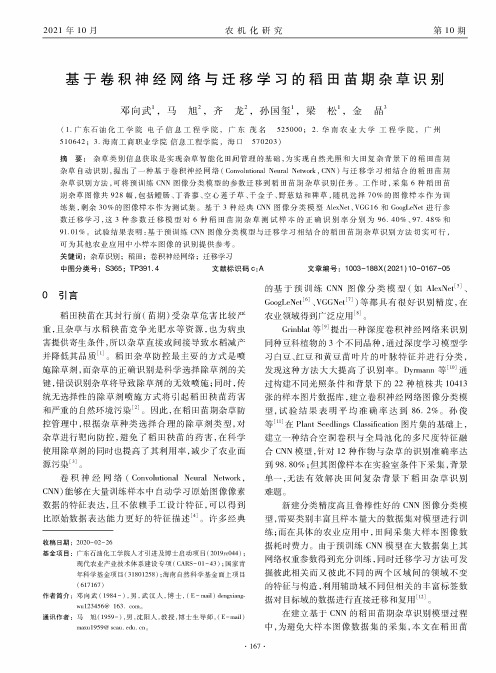
基于卷积神经网络与迁移学习的稻田苗期杂草识别邓向武（，马旭2，齐龙2,孙国玺（，梁松（,金晶3（6广东石油化工学院电子信息工程学院，广东茂名525000；2.华南农业大学工程学院，广州510642；3.海南工商职业学院信息工程学院，海口570203）摘要：杂草类别信息获取是实现杂草智能化田间管理的基础，为实现自然光照和大田复杂背景下的稻田苗期杂草自动识别，提出了一种基于卷积神经网络（Co/voluLo/sl Nexrvi Network,CNN）与迁移学习相结合的稻田苗期杂草识别方法，可将预训练CNN图像分类模型的参数迁移到稻田苗期杂草识别任务。

工作时，采集6种稻田苗期杂草图像共928幅，包括鳢肠、丁香蓼、空心莲子草、千金子、野慈姑和稗草，随机选择70%的图像样本作为训练集，剩余30%的图像样本作为测试集。

基于3种经典CNN图像分类模型AlexNc—VGG16和GoogLeNet进行参数迁移学习，这3种参数迁移模型对6种稻田苗期杂草测试样本的正确识别率分别为96.40%、97.48%和71.41%o试验结果表明：基于预训练CNN图像分类模型与迁移学习相结合的稻田苗期杂草识别方法切实可行，可为其他农业应用中小样本图像的识别提供参考。

关键词：杂草识别；稻田；卷积神经网络；迁移学习中图分类号：S365；TP391.4文献标识码c：A文章编号：1003-188X（2021）10-0167-050引言稻田秧苗在其封行前（苗期）受杂草危害比较严重，且杂草与水稻秧苗竞争光肥水等资源，也为病虫害提供寄生条件,所以杂草直接或间接导致水稻减产并降低其品质［］。

稻田杂草防控最主要的方式是喷施除草剂，而杂草的正确识别是科学选择除草剂的关键,错误识别杂草将导致除草剂的无效喷施；同时，传统无选择性的除草剂喷施方式将引起稻田秧苗药害和严重的自然环境污染⑵。

因此，在稻田苗期杂草防控管理中，根据杂草种类选择合理的除草剂类型，对杂草进行靶向防控，避免了稻田秧苗的药害，在科学使用除草剂的同时也提高了其利用率,减少了农业面源污染⑻。

Uniform (Continuous) DistributionQuantile-Quantile Plots Empirical Cumulative Distribution Function (CDF)Hidden Markov Model Functions New Functions for Extreme Value DistributionsStatistics Toolbox wblcdfWeibull cumulative distribution function (cdf)SyntaxP = wblbcdf(X, A, B)[P, PLO, PUP] = wblcdf(X, A, B, PCOV, alpha)DescriptionP = wblbcdf(X, A, B) computes the cdf of the Weibull distribution with scale parameter A and shape parameter B, at each of the values in X. X, A, and B can be vectors, matrices, or multidimensional arrays that all have the same size. A scalar input is expanded to a constant array of the same size as the other inputs. The default values for A and B are both 1. The parameters A and B must be positive.[P, PLO, PUP] = wblcdf(X, A, B, PCOV, alpha) returns confidence bounds for P when the input parameters A and B are estimates. PCOV is the 2-by-2 covariance matrix of the estimated parameters. alpha has a default value of 0.05, and specifies 100(1 - alpha)% confidence bounds. PLO and PUP are arrays of the same size as P containing the lower and upper confidence bounds.The function wblcdf computes confidence bounds for P using a normal approximation to the distribution of the estimateand then transforms those bounds to the scale of the output P. The computed bounds give approximately the desired confidence level when you estimate m u, sigma, and PCOV from large samples, but in smaller samples other methods of computing the confidence bounds might be more accurate.The Weibull cdf isExamplesWhat is the probability that a value from a Weibull distribution with parameters a = 0.15 and b =0.8 is less than 0.5?probability = wblcdf(0.5, 0.15, 0.8)probability =0.9272How sensitive is this result to small changes in the parameters?[A, B] = meshgrid(0.1:0.05:0.2,0.2:0.05:0.3);probability = wblcdf(0.5, A, B)probability =vartestn wblfitwblcdf wblinvStatistics Toolbox wblinvInverse of the Weibull cumulative distribution functionSyntaxX = wblinv(P, A, B)[X, XLO, XUP] = wblinv(P, A, B, PCOV, alpha)DescriptionX = wblinv(P, A, B) returns the inverse cumulative distribution function (cdf) for a Weibull distribution with scale parameter A and shape parameter B, evaluated at the values in P. P, A, and B can be vectors, matrices, or multidimensional arrays that all have the same size. A scalar input is expanded to a constant array of the same size as the other inputs. The default values for A and B are both 1.[X, XLO, XUP] = wblinv(P, A, B, PCOV, alpha) returns confidence bounds for X when the input parameters A and B are estimates. PCOV is a 2-by-2 matrix containing the covariance matrix of the estimated parameters. alpha has a default value of 0.05, and specifies 100(1 - a lpha)% confidence bounds. XLO and XUP are arrays of the same size as X containing the lower and upper confidence bounds.The function wblinv computes confidence bounds for X using a normal approximation to the distribution of the estimatewhere q is the P th quantile from a Weibull distribution with scale and shape parameters both equal to 1. The computed bounds give approximately the desired confidence level when you estimate mu, sigma, and PCOV from large samples, but in smaller samples other methods of computing the confidence bounds might be more accurate.The inverse of the Weibull cdf isExamplesThe lifetimes (in hours) of a batch of light bulbs has a Weibull distribution with parameters a = 200 and b = 6. What is the median lifetime of the bulbs?life = wblinv(0.5, 200, 6)life =188.1486What is the 90th percentile?life = wblinv(0.9, 200, 6)life =wblfit wbllikewblinv wblpdfwbllike wblplotwblpdf wblrndwblplot wblstatwblrnd wishrnd。