K-short Reconstruction using the Full and Fast Simulations

Overview of CMS virtual data needsDecember20001IntroductionThis document was put together to act as CMS input into the Griphyn Architecture meeting on De-cember20,2000.It is a high-level overview that tries to be short rather than complete.Structure of this document:Brief overview of CMS and its physicsCMS virtual data description2005vs.current needs and activitiesReferences to some other documents that may be of interest2Brief overview of CMS and its physics2.1CMSThe CMS experiment is a high energy physics experiment located at CERN,that will start data tak-ing in2005.The CMS detector(figure1)is one of the two general purpose detectors of the LHC accelerator.It is being designed and built,and will be used,by a world-wide collaboration,the CMS collaboration,that currently consists of some2200people in145institutes,divided over30countries. In future operation,the LHC accelerator lets two bunches of particles cross each other inside the CMS detector40.000.000times each second.Every bunch contains some protons.In every bunch crossing in the detector,on average20collisions occur between two protons from opposite bunches.A bunch crossing with collisions is called an event.Figure2shows an example of an event.Note that the picture of the collision products is very complex,and represents a lot of information:CMS has15 million individual detector channels.The measurements of the event,done by the detector elements in the CMS detector,are called the’raw event data’.The size of the raw event data for a single CMS event is about1MB(after compression using‘zero suppression’).Figure1:The CMS detector.Of the40.000.000events in a second,some100are selected for storage and later analysis.This selection is done with a fast real-timefiltering system.Data analysis is done interactively,by CMS physicists working all over the world.Apart from a central data processing system at CERN,there will be some5–10regional centres all over the world that will support data processing.Further processing may happen locally at the physicist’s home institute,maybe also on the physicist’s desktop machine. The1MB’raw event’data for each event is not analyzed directly.Instead,for every stored raw event,a number of summary objects are computed.These summary objects range in size from a100 KB’reconstructed tracks’object to a100byte’event tag’object,see section3.1for details.This summary data will be replicated widely,depending on needs and capacities.The original raw data will stay mostly in CERN’s central robotic tape store,though some of it may be replicated too.Due to the slowness of random data access on tape robots,the access to raw data will be severely limited.2.2Physics analysisBy studying the momenta,directions,and other properties of the collision products in the event, physicists can learn more about the exact nature of the particles and forces that were involved in the collision.For example,to learn more about Higgs bosons,one can study events in which a collision produced a Higgs boson that then decayed into four charged leptons.(A Higgs boson decays almost immediately after creation,so it cannot be observed directly,only its decay products can be observed.)A Higgs boson analysis effort can therefore start with isolating the set of events in which four charged leptons were produced.Not all events in this set correspond to the decay of a Higgs boson:there are many other physics processes that also produce charged leptons.Therefore,subsequent isolation steps are needed,in which’background’events,in which the leptons were not produced by a decaying Higgs boson,are eliminated as much as possible.Background events can be identified by looking at other observables in the event record,like the non-lepton particles that were produced,or the momenta ofFigure2:A CMS event(simulation).particles that left the collision point.Once enough background events have been eliminated,some important properties of the Higgs boson can be determined by doing a statistical analysis on the set of events that are left.The data reduction factor in physics analysis is enormous.Thefinal event set in the above example may contain only a few hundreds of events,selected from the events that occurred in one year in the CMS detector.This gives a data reduction factor of about1in.Much of this reduc-tion happens in the real-timefilter before any data is stored,the rest happens through the successive application of‘cut predicates’to the stored events,to isolate ever smaller subsets.3CMS virtual data description3.1Structure of event dataCMS models all its data in terms of objects.We will call the objects that represent event data,or summaries of event data,‘physics objects’.The CMS object store will contain a number of physics objects for each event,as shown infigure3.In a Griphyn context,on can think of each object infigure3as a materialized virtual data object.Among themselves,the objects for each event form a hierarchy.At higher levels in the hierarchy,the objects become smaller,and can be thought of as holding summary descriptions of the data in the objects ata lower level.By accessing the smallest summary object whenever possible,physicists can save bothFigure3:Example of the physics objects present for two events.The numbers indicateobject sizes.The reconstructed object sizes shown reflect the CMS estimates in[1].Thesum of the sizes of the raw data objects for an event is1MB,this corresponds to the1MBraw event data specified in[1].CPU and I/O resources.At the lowest level of the hierarchy are raw data objects,which store all the detector measurements made at the occurrence of the event.Every event has about1MB of raw data in total,which is partitioned into objects according to some predefined scheme that follows the physical structure of the detector.Above the raw data objects are the reconstructed objects,they store interpretations of the raw data in terms of physics processes.Reconstructed objects can be created by physicists as needed, so different events may have different types and numbers of reconstructed(materialized)objects.At the top of the hierarchy of reconstructed objects are event tag objects of some100bytes,which store only the most important properties of the event.Several versions of these event tag objects can exist at the same time.3.2Data dependenciesTo interpretfigure3in terms of virtual data,one has to make visible the way in which each of these objects was computed.This is done infigure4:it shows the data dependencies for objects infigure3. Note that the‘raw’objects are not computed,they correspond to detector measurements.Infigure3an arrow from to signifies that the value of depends on.The grey boxes represent physics algorithms used to compute the object:note that these all have particular versions.The lower-most grey box represents some’calibration constants’that specify the configuration of the detector over time.Calibration is outside of the scope of this text.Note that,usually,there is only one way in which a requested CMS virtual data product can be computed.This in contrast with LIGO,where often many ways to compute a product are feasible, and where one challenge to the scheduler is tofind the most efficient way.Figure4:Data dependencies for some of the objects infigure3.An arrow from tosignifies that the value of depends on.The grey boxes represent physics algorithmsused to compute the objects,and some’calibration constants’used by these algorithms.3.3Encoding data dependency specificsAs is obvious fromfigure4,the data dependencies for any physics object can become very complex. Note however that,for the two events infigure4,the dependency graphs are similar.It is possible to make a single big dependency graph,in a metadata repository,that captures all possible dependencies between the physics objects of every event.Figure5shows such a metadata graph for the events in figure4.graph.The numbers in the nodes representing physics objects are globally unique typenumbers.In the metadata graph,the physics objects are replaced by unique type numbers.These numbers can be used to represent the particular data dependencies and algorithms that went into the computation of any reconstructed object.A CMS virtual data addressing system could use the type numbers as keysin a transformation catalog that yields instructions on how to compute any virtual physics object. 3.4Virtual data object identificationIn CMS it is possible to uniquely identify every(virtual or real)physics object by a tuple(event ID,type number).Thefirst part of the tuple is the(unique)identifier of the event the object belongs to,the second the unique identifier of the corresponding location in the object dependency graph discussed above.3.5Importance of physics objects relative to other data productsBesides the physics objects as shown infigure3,where each object holds data about a single event only,CMS will also work with data products that describe properties of sets of events.There will be several types of such products with names like‘calibration data’,‘tag collections’,‘histograms’,‘physics papers’,etc.However in terms of data volume these products will be much less significant than the physics objects.In terms of virtual data grids,it is believed that the big challenge for CMS lies in making these grids compute and deliver physics objects to‘physics analysis jobs’,where these physics jobs can output relatively small data products like histograms that need not necessarily be managed by the grid.3.6Typical physics jobA typical job computes a function value for every event in some set,and aggregates the function results.In contrast with LIGO,in CMS the will generally be a very sparse subset of the events taken over a very long time interval.To compute,the values of one or more virtual data products for this event are needed.Generally,for every event will request the same product(s), products with the same‘type numbers’.In a high energy physics experiment,there is no special correlation between the time an event collision took place and any other property of the event:events with similar properties are evenly distributed over the time sequence of all events.In physics analysis jobs,events are treated as completely inde-pendent from each other.If function results are aggregated,the aggregation function does not depend on the order in which the function results are fed to it.Thus,from a physics standpoint,the order of traversal of a job event set does not influence the job result.3.7CMS virtual data grid characteristicsWhen comparing the grid requirements of a high energy physics experiment like CMS with the re-quirements of LIGO and SDSS,the points which are characteristic for CMS are:Not very large but extremely large amounts of data.Large amount of CPU power needed to derive needed virtual data products.The above two imply that fault tolerant facilities for the mass-materialization of virtual data products on a large and very distributed system are essential.Baseline virtual data model does not have virtual data products that aggregate data from multiple events,so the model looks relatively simple from a scheduling standpoint.A requested set of data products generally corresponds to a very sparse subset of the eventstaken over a very long time interval.42005vs.current needs and activitiesThe preceding sections talk about the CMS data model and data analysis needs when the experiment is running from2005on.This section discusses current and near-future needs and activities,and contrasts these to the2005needs.Currently CMS is performing large-scale simulation efforts,in which physics events are simulated as they occur inside a simulation of the CMS detector.These simulation efforts support detector design and the design of the real-time eventfiltering algorithms that will be used when CMS is running.The simulation efforts are in the order of hundreds of CPU years and terabytes of data.These simula-tion efforts will continue,and will grow in size,up to2005and then throughout the lifetime of the experiment.The simulation efforts and the software R&D for CMS data management are seen as strongly intertwined and complementary activities.In addition to performing grid-related R&D in the context of several projects,CMS is also already using some grid-type software‘in production’for its simulation efforts.Examples of this is the use of Condor-managed CPU power in some large-scale simulation efforts,and the use of some Globus components by GDMP[7],which is a software system developed by CMS that is currently being used in production to replicatefiles with simulation results in the wide-area.CMS simulation efforts currently still rely to a large extent on hand-coded shell and perl scripts, and the careful manual mapping of hardware resources to tasks.As more grid technology becomes available,CMS will be actively looking to use it in its simulation efforts,both as a way to save manpower and as a means to allow for greater scalability.On the grid R&D side,the CMS simulation codes could also be used inside testbeds that evaluate still-experimental grid technologies.It thus makes sense to look more closely here at the exact properties of the CMS simulation efforts,and how these differ from those of the2005CMS virtual data problem.Each individual CMS simulation run can be modeled as a definition of a set of virtual data products and a request to materialize them into a set offiles.Current CMS simulation runs have a batch nature, not an interactive nature.Each large run generally at least takes a few days to plan,with several people getting involved,and then at least few weeks to execute.At most some tens of runs will be in progress at the same time.So there is a huge contrast with the2005situation,where CMS data processing requirements are expected to be dominated by‘chaotic’interactive physics analysis workloads generated by hundreds of physicists working independently.Also,in contrast to the2005 workloads,requests for the data in sparse subsets of(simulated)event datasets will be rare,if they occur at all.Simulated event sets can be,and are,generated in such a way that events likely to be requested together are created together in the same databasefile or set of databasefiles.Therefore, to support simulation runs in the near future,it would be possible to use a virtual data system that works at the granularity offiles,rather than thefiner granularity of events or objects.Going towards 2005,the data creation and transport needs of the CMS simulation exercises are expected to become increasingly‘chaotic’andfine-grained,but the exact pace at which change will happen is currently not known.CMS currently has two distinct simulation packages.The Fortran-based CMSIM software takes care of thefirst steps in a full simulation chain.It producesfiles which are then read by the C++-based ORCA software.CMSIM usesflatfiles in the‘fz’format for its output,ORCA data storage is done using the Objectivity object database.CMSIM will be phased out in the next few years,it will be replaced by more up-to-date simulation codes using the C++-based next-generation GEANT4physics simulation library.As targets for the use in virtual data testbeds,CMSIM and ORCA each have their own strengths and weaknesses.In CMSIM,each simulation run produces one outputfile based on a set of runtime parameters.This yields a virtual data model that is almost embarrassingly simple, a data model of‘virtual outputfiles’,with eachfile having a runtime parameter set as its unique signature,and no dependencies betweenfiles.CMSIM is very portable and can be run on almost any platform.Installing the CMSIM software is not a major job.The simulations involving ORCA display a much more complicated pattern of data handling in which intermediate products appear[3], and a corresponding virtual data model would be much more complex,and more representative of the 2005situation.The ORCA software is under rapid development,with cycles of a few months or less. ORCA is only supported on Linux and Solaris,and currently takes considerable effort and expertise to install.Work on more automated installation procedures is underway.5References to some other documents that may be of interestThe CMS Computing Technical Proposal[1],written in1996,is still a good source of overview mate-rial.More recent sources are[5],which has material on CMS physics and its software requirements, and[2]which has more details about the CMS2005data model and expected access patterns.A short write-up on CMSIM and virtual data is[6].More details on simulations using ORCA are in[3]and[4].References[1]CMS Computing Technical Proposal.CERN/LHCC96-45,CMS collaboration,19December1996.[2]Koen Holtman,Introduction to CMS from a CS viewpoint.21Nov2000.http://home.cern.ch/kholtman/introcms.ps[3]David Stickland.The Design,Implementation and Deployment of Functional Prototype OOReconstruction Software for CMS.The ORCA project.http://chep2000.pd.infn.it/abst/abs。

医疗医务标准化CT血管重建软件在输尿管病变标准化诊断中的应用■ 车立昆 雷舟杰 栾 海 冯翼飞（联勤保障部队北戴河康复疗养中心 健康管理部医学影像科）摘 要：目的：探讨CT血管重建软件在输尿管病变标准化诊断中的应用价值。

材料和方法：47例输尿管病变患者，一组24例为CT尿路造影检查（CTU），二组23例为普通CT平扫检查，所有图像传输至AW4.6工作站并选择血管重建软件进行CPR（曲面重建）尿路成像。

结果：47例输尿管病变，输尿管癌10例，先天畸形15例，输尿管结石12例，输尿管炎8例，输尿管息肉1例，输尿管吻合口狭窄1例，CT血管重建软件CPR尿路成像操作时间短，所有成像轨迹可纠正检验，减少以往人为操作带来的误差。

结论：CT血管重建技术生成CPR优势较大，对输尿管病变的显示和标准化诊断有优越性，具有非常高的临床实用价值。

关键词：输尿管病变，X线计算机，血管重建，曲面重建DOI编码：10.3969/j.issn.1002-5944.2023.24.069Application of CT Vascular Reconstruction Software in StandardizedDiagnosis of Ureteral DiseasesCHE Li-kun LEI Zhou-jie LUAN Hai FENG Yi-fei（Medical Imaging Department, Health Management Department, Beidaihe Rehabilitation Center, Joint Logistic Support Force）Abstract:Objective: To explore the application value of CT vascular reconstruction software in the standardized diagnosis of ureteral diseases. Methods: There were 47 patients with ureteral diseases. One group consisted of 24 patients who underwent CT urography (CTU), and the other group consisted of 23 patients who underwent conventional CT plain scan. All images were transmitted to the AW4.6 workstation and curved surface reconstruction (CPR) urography was performed using vascular reconstruction software. Results: The results showed that the 47 cases of ureteral diseases included 10 cases of ureteral cancer, 15 cases of congenital malformations, 12 cases of ureteral stones, 8 cases of ureteritis, 1 case of ureteral polyp, and 1 case of ureteral anastomotic stenosis. The CT vascular reconstruction software CPR urography had a short operating time for urinary tract imaging, and all imaging trajectories could be corrected and tested, reducing errors caused by previous human operations. Conclusion: CT vascular reconstruction technology has a signifi cant advantage in generating CPR, and has advantages in displaying and standardizing the diagnosis of ureteral diseases, which has very high clinical practical value.Keywords: ureteropathy, X-ray computer, vascular reconstruction, curved surface reconstruction输尿管等具有管腔结构的器官走形弯曲及毗邻结构较复杂，从而影响这些具有管腔性结构的器官病变的检出率[1]。

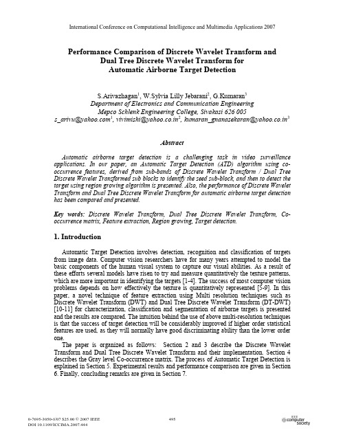
International Conference on Computational Intelligence and Multimedia Applications 2007Performance Comparison of Discrete Wavelet Transform andDual Tree Discrete Wavelet Transform forAutomatic Airborne Target DetectionS.Arivazhagan1, W.Sylvia Lilly Jebarani2, G.Kumaran3Department of Electronics and Communication EngineeringMepco Schlenk Engineering College, Sivakasi 626 005s_arivu@1, vivimishi@yahoo.co.in2, kumaran_gnanasekaran@yahoo.co.in3AbstractAutomatic airborne target detection is a challenging task in video surveillance applications. In our paper, an Automatic Target Detection (ATD) algorithm using co-occurrence features, derived from sub-bands of Discrete Wavelet Transform / Dual Tree Discrete Wavelet Transformed sub blocks to identify the seed sub-block, and then to detect the target using region growing algorithm is presented. Also, the performance of Discrete Wavelet Transform and Dual Tree Discrete Wavelet Transform for automatic airborne target detection has been compared and presented.Key words: Discrete Wavelet Transform, Dual Tree Discrete Wavelet Transform, Co-occurrence matrix, Feature extraction, Region growing, Target detection.1. IntroductionAutomatic Target Detection involves detection, recognition and classification of targets from image data. Computer vision researchers have for many years attempted to model the basic components of the human visual system to capture our visual abilities. As a result of these efforts several models have risen to try and measure quantitatively the texture patterns, which are more important in identifying the targets [1-4]. The success of most computer vision problems depends on how effectively the texture is quantitatively represented [5-9]. In this paper, a novel technique of feature extraction using Multi resolution techniques such as Discrete Wavelet Transform (DWT) and Dual Tree Discrete Wavelet Transform (DT-DWT) [10-11] for characterization, classification and segmentation of airborne targets is presented and the results are compared. The intuition behind the use of above multi-resolution techniques is that the success of target detection will be considerably improved if higher order statistical features are used, as they will normally have good discriminating ability than the lower order one.The paper is organized as follows: Section 2 and 3 describe the Discrete Wavelet Transform and Dual Tree Discrete Wavelet Transform and their implementation. Section 4 describes the Gray level Co-occurrence matrix. The process of Automatic Target Detection is explained in Section 5. Experimental results and performance comparison are given in Section 6. Finally, concluding remarks are given in Section 7.2. Discrete wavelet transformThe Discrete Wavelet Transform (DWT) analyzes the signal at different frequency bands with different resolutions by decomposing the signal into a coarse approximation and detail information. The DWT employs two sets of functions, called scaling functions and wavelet functions, which are associated with low pass and high pass filters, respectively. In order to decompose an image, first, the low pass filter (h) is applied for each row of data and subsequently down sampled by 2, thereby getting the low frequency components of the row. Then, the high pass filter (g) is applied for the same row of data, subsequently down sampled by a factor 2 to get high frequency components, and placed by the side of low pass components. This procedure is done for all rows. Down sampling is done to satisfy Nyquist’s rule, since the signal now has a highest frequency of /2πradians instead of πafter filtering. Next, the filtering is done for each column of the intermediate row decomposed data. The resulting two-dimensional array of coefficients contains four bands of data, each labeled as LL1 (low-low), LH1 (low-high), HL1 (high-low) and HH1 (high-high), corresponding to first level of image decomposition. The LL1 band can be further decomposed in the same manner for second level of decomposition. This can be done up to any level, thereby resulting in a pyramidal decomposition. The one level decomposed image is represented in Figure 1 (a) andFigure 1. Image Decomposition using DWT; (a) One level DWT(b) Filter bank structure for one level of Image decompositionIn our implementation, the target image is subjected to one level of DWT decomposition and the features derived from three detail sub-bands are used for target detection.3. Dual tree discrete wavelet transformThe standard DWT and its extensions suffer from two or more serious limitations. They are: (i) Lack of shift invariance , which means that small shifts in the input signal can cause major variations in the distribution of energy between DWT coefficients at different scales and (ii) Poor directional selectivity for diagonal features, because the wavelet filters are separable and real.A well-known way of providing shift invariance is to use the undecimated form of the dyadic filter tree. However this still suffers from substantially increased computation requirements compared to the fully decimated DWT and also exhibits high redundancy in the(a) 2 1 2 0 1 0 2 1 1 2 0 1 2 2 0 1 2 2 0 1 2 0 1 0 1(a)(b)output information, making subsequent processing expensive too. A more computationally efficient approach to shift invariance is Dual-Tree Discrete Wavelet Transform (DT-DWT). Furthermore, the DT-DWT also gives much better directional selectivity when filtering multidimensional signals. In summary, it has the properties, such as (i) Approximate shift invariance, (ii) Good directional selectivity in 2-dimensions and (iii) Perfect reconstruction (PR) using short linear-phase filtersDT-DWT use complex-valued filtering (analytic filter) that decomposes the real/complex signals into real and imaginary parts in transform domain. When an image is subjected to one level DT-DWT decomposition, it results in 16 sub bands as shown in Figure 2 (a). These 16 sub bands arise from separable applications of real and imaginary filters on horizontal and vertical directions respectively as shown in Figure 2 (b). Here, each block, identical to standard 2D-DWT results in 4 sub-bands where h is the set of filters {h 0, h 1} and g is the set of filters {g 0, g 1}. The filters h 0, h 1 are real valued low pass and high pass filters respectively for real tree and g 0, g 1 are the corresponding filters for imaginary tree and x and y represent row and column directions respectively for filtering. The overall 2-D dual-tree structure is 4-times redundant than the standard 2-D DWT. In our implementation, features are derived from 12Figure 2. One level 2D DT- DWT;a) Image Decomposition; (b) Filter bank structure4. Gray level co-occurrence matrixWhen a digital image is represented in the form of matrix whose elements indicate the intensity level of the image at that point for the gray level images and the level varies from 0 to 255.Figure 3. Derivation of Co-occurrence matrix(a) A 5x5 image with three gray levels 0, 1 and 2; (b) Co-occurrence matrixorientation (c) The gray level Co-occurrence matrix for d = (1, 1).The gray-level co-occurrence matrix C [i, j] is defined by first specifying a displacement d = (dx, dy) and counting all pairs of pixels separated by d having gray-levels i, j [2]. The dx and dy represent the displacement in x and y directions respectively. For example, consider the simple 55× image having gray levels 0, 1 and 2 as shown in Figure 3 (a). Since, there are only three gray levels, C [i, j] is a 33× matrix. Let the position operator is specified as (1, 1), which has the interpretation: one pixel to the right and one pixel below. For example, there are three pairs of pixels having values [2, 1] which are separated by the specified distance, and hence the entry C[2, 1] has a value of 3. The complete matrix C [i,j] is shown in Figure 3 (c).5. Automatic target detection systemThe various processes involved in the Automatic Target Detection system are shown in Figure 4. The image of size N N × is individually considered as having a number of non-overlapping and adjacent sub-blocks of size n n × where n<N . Starting from the top-left corner5.1 Feature extraction A significant Co-occurrence feature namely contrast is derived from detail sub-bands of DWT / DT-DWT decomposed sub blocks of the original image using the equation (1). This feature is further used in target detection to identify the seed sub block for subsequent region growing process.∑=−=n j i j i C j i contrast 0,),(22)( (1)where C(i, j) is the Co-occurrence matrix elements.5.2 Seed identification and region growingOnce the contrast value of all the sub blocks are computed, the sub block having the maximum contrast value is identified as the ‘seed’ sub block for subsequent region growing. The region growing algorithm merges those neighboring sub blocks which are having a contrast difference less than the threshold. The threshold is computed from the mean of the difference of the contrast values between the ‘seed’ and its eight neighbors. The region growing algorithm is iteratively applied till new sub blocks are no longer merged along with the seed. As the merging process gets completed, a bounded rectangle encompasses the target with a mark on the centroid of the target.6. Experimental results and performance comparisonOur algorithm using DWT and DT-DWT is applied on 6 different airborne target still images of various sizes under both cloudy and clear environment and the experimental results obtained for the same are shown in Table 1. The table shows the original images, Target identified images using DWT and DT-DWT and the corresponding execution times. Though the size of the sub block is dependent on the size of the target, a sub block size of 32 x 32 gave promising results irrespective of the size of the targets in the images chosen for experimentation.Table 1. Performance Comparison of Target Detection using DWT and DT-DWTSl. No Input Image Target Identified image using DWT Target Identified image using DT-DWT Execution time in Seconds for DWT Execution time inSeconds forDT-DWT10.171 0.57820.140 0.45330.125 0.35940.203 0.81250.140 0.48460.156 0.484From the table, it is observed that both DWT and DT-DWT based algorithms performs well on all targets, irrespective of its size and orientation. Also, it is found that the average computation time using C language program for DWT is 0.155 second while for DT-DWT it is 0.528second.7. ConclusionBoth the Multi resolution techniques detect the target irrespective of their size, perspective and background. Compared to DWT, application of DT-DWT results in better spatial localization. This improvement is mainly due to deriving co-occurrence feature namely contrast, from 12 detail sub-bands against three sub-bands in DWT, which results in increased computational time.AcknowledgementThis project is funded by Armament Research Board, Defense Research Development Organization (DRDO), New Delhi. The authors are expressing their sincere thanks to the Management and Principal, Mepco Schlenk Engineering College, Sivakasi for their constant encouragement and support.References[1]. F.Espinal, B.D.Jawerth and T.Kubota, “Wavelet based fractal signature analysis for automatic targetrecognition”, Journal of Society of Photo-Optical Instrumentation Engineers, Vol. 37. No.1, 1998, pp. 166-174.[2].R.M.Haralick, K.Shanmugam and I.Dinstein, “Texture features for image classification”, IEEETransactions on System, Man, Cybernatics, Vol.8, No.6, 1973, pp. 610-621.[3].J.Sklansky, “Image segmentaion and feature extraction”, IEEE Transactions on System, Man, Cybernatics,Vol.8, No.4, 1978, pp. 237-247.[4].L.S.Davis, S.A.Johns and J.K.Aggarwal, “Texture analysis using generalized co-occurrence matrices”,IEEE Transactions on Pattern Analysis and Machine Intelligence, Vol.1, No.3, 1979, pp. 251–259.[5].M.Unser and M.Eden, “Multiresolution feature extraction and selection for texture segmentation”, IEEETransactions on Pattern Analysis and Machine Intelligence, Vol. 11, No.7, 1989, pp. 717 – 728.[6].Tianhorng Chang and C C Jay Kuo, “Texture analysis and classification with tree-structured wavelettransform”, IEEE Transactions on Image processing, Vol.2, No.4, 1993, pp. 429-440.[7].G Van de Wouwer, P Schenders and D Van Dyek, “Statistical texture characterization from discretewavelet representation”, IEEE Transactions on Image processing, Vol.8, No.4, 1999, pp. 592-598.[8].S.Arivazhagan and L.Ganesan, “Texture Classification using Wavelet Transform”, Pattern RecognitionLetters, Vol.24, No. 9-10, 2003, pp. 1513-1521.[9]. A.Howard, C.Padgett and K.Brown, “Real Time Intelligent Target Detection and Analysis with MachineVision”, Proc. of 3rd International Symposium on Intelligent Automation and Control, World Automation Congress, 2000.[10].S erkan Hat.ipoglu, Sanjit K. Mit.ra and Nick Kingsbury, “Texture classification using Dual-Tree ComplexWavelet Transform”, IEE Conference on Image Processing and its Applications, 465, 1999, pp. 344-347.[11].P anchamkumar D Shukla, “Complex Wavelet Transforms and their Applications”, M.Phil.Thesis, SignalProcessing Division, Department of Electronic and Electrical Engineering, University of Strathclyde, Glasgow G11XW, Scotland, United Kingdom, 2003.。

摘要随着表面贴装技术（Surface Mounting Technology，SMT）兴起，电子元器件逐渐趋于小型化、密集化。

作为SMT第一道工序的锡膏印刷，若能实施全面检测，例如漏印、缺锡、少锡、偏移和连桥等，避免少锡或者缺锡导致虚焊，偏移和连桥形成短路等问题，这不仅可以在电子印刷电路板（Printed Circuit Board，PCB）的早期发现产品不良趋势，而且对于生产效率的提高和返修成本的降低等具有重要意义。

基于计算机视觉检测理论的锡膏印刷图像检测技术及设备，借助于外部的光栅、激光光源，通过电荷耦合器件（Charged Coupled Device，CCD）相机成像，按不同算法生成被测焊点形貌，利用锡膏印刷图像的高度、面积、体积特征，可以及时发现锡膏印刷过程中的缺陷和不足。

本文调研与分析了激光三角测量和相位光栅测量（Phase Measuring Profilometry，PMP）的原理及技术方法，针对三维锡膏检测设备虽利用了激光三角原理的锡膏检测仪（Solder Paste Inspection，SPI）速度快，三维效果好，但重复精度低，检测结果受外界震动和传动装置的震动影响大以及相位光栅测量方法需要结构光照明，虽重复性和再现性好，但测量的锡膏体积比真实锡膏体积偏小等情况，提出了基于双目视觉的三维锡膏检测方法。

首先，构建了灵活可调的三维锡膏检测系统平台。

平台底座采用了全新的大理石，保证了机身的坚固和稳定性。

传输系统采用了高速运动控制系统，设计了插补方式实现的精确轨迹运动。

照明系统由高亮度的LED（Light Emitting Diode）经特殊的球面结构形成均匀扩散光，防止电路板图像表面形成的漫反射，此为清晰的成像提供了保障。

相机系统采用了基于两点参考法的平场校正，消除了CCD 成像的非均匀性，通过白平衡处理，使得拍摄的PCB图像呈现真实的色彩。

为了减少扫描次数，降低对机械部件的磨损，延长系统寿命，使其可靠稳定运行，相机视场最大可设置为44mm⨯420mm，采集图像所包含的像素为3648⨯13750≈500万。

2021⁃04⁃10计算机应用,Journal of Computer Applications2021,41(4):1012-1019ISSN 1001⁃9081CODEN JYIIDU http ：//基于注意力融合网络的视频超分辨率重建卞鹏程，郑忠龙*，李明禄，何依然，王天翔，张大伟，陈丽媛（浙江师范大学数学与计算机科学学院，浙江金华321004）（∗通信作者电子邮箱zhonglong@ ）摘要：基于深度学习的视频超分辨率方法主要关注视频帧内和帧间的时空关系，但以往的方法在视频帧的特征对齐和融合方面存在运动信息估计不精确、特征融合不充分等问题。

针对这些问题，采用反向投影原理并结合多种注意力机制和融合策略构建了一个基于注意力融合网络（AFN ）的视频超分辨率模型。

首先，在特征提取阶段，为了处理相邻帧和参考帧之间的多种运动，采用反向投影结构来获取运动信息的误差反馈；然后，使用时间、空间和通道注意力融合模块来进行多维度的特征挖掘和融合；最后，在重建阶段，将得到的高维特征经过卷积重建出高分辨率的视频帧。

通过学习视频帧内和帧间特征的不同权重，充分挖掘了视频帧之间的相关关系，并利用迭代网络结构采取渐进的方式由粗到精地处理提取到的特征。

在两个公开的基准数据集上的实验结果表明，AFN 能够有效处理包含多种运动和遮挡的视频，与一些主流方法相比在量化指标上提升较大，如对于4倍重建任务，AFN 产生的视频帧的峰值信噪比（PSNR ）在Vid4数据集上比帧循环视频超分辨率网络（FRVSR ）产生的视频帧的PSNR 提高了13.2%，在SPMCS 数据集上比动态上采样滤波视频超分辨率网络（VSR -DUF ）产生的视频帧的PSNR 提高了15.3%。

关键词：超分辨率；注意力机制；特征融合；反向投影；视频重建中图分类号：TP391.4文献标志码：AAttention fusion network based video super -resolution reconstructionBIAN Pengcheng ，ZHENG Zhonglong *，LI Minglu ，HE Yiran ，WANG Tianxiang ，ZHANG Dawei ，CHEN Liyuan（College of Mathematics and Computer Science ，Zhejiang Normal University ，Jinhua Zhejiang 321004，China ）Abstract:Video super -resolution methods based on deep learning mainly focus on the inter -frame and intra -frame spatio -temporal relationships in the video ，but previous methods have many shortcomings in the feature alignment and fusion of video frames ，such as inaccurate motion information estimation and insufficient feature fusion.Aiming at these problems ，a video super -resolution model based on Attention Fusion Network （AFN ）was constructed with the use of the back -projection principle and the combination of multiple attention mechanisms and fusion strategies.Firstly ，at the feature extraction stage ，in order to deal with multiple motions between neighbor frames and reference frame ，the back -projection architecture was used to obtain the error feedback of motion information.Then ，a temporal ，spatial and channel attention fusion module was used to perform the multi -dimensional feature mining and fusion.Finally ，at the reconstruction stage ，the obtained high -dimensional features were convoluted to reconstruct high -resolution video frames.By learning different weights of features within and between video frames ，the correlations between video frames were fully explored ，and an iterative network structure was adopted to process the extracted features gradually from coarse to fine.Experimental results on two public benchmark datasets show that AFN can effectively process videos with multiple motions and occlusions ，and achieves significant improvements in quantitative indicators compared to some mainstream methods.For instance ，for 4-times reconstruction task ，the Peak Signal -to -Noise Ratio （PSNR ）of the frame reconstructed by AFN is 13.2%higher than that of Frame Recurrent Video Super -Resolution network （FRVSR ）on Vid4dataset and 15.3%higher than that of Video Super -Resolution network using Dynamic Upsampling Filter （VSR -DUF ）on SPMCS dataset.Key words:super -resolution;attention mechanism;feature fusion;back -projection;video reconstruction文章编号：1001-9081（2021）04-1012-08DOI ：10.11772/j.issn.1001-9081.2020081292收稿日期：2020⁃08⁃24；修回日期：2020⁃09⁃18；录用日期：2020⁃10⁃13。

My smmr hols wr CWOT.B4, we usd 2 go 2 NY 2C my bro, his GF & thr 3 :-@ kds FTF.ILNY, its gr8.Bt my Ps wr so {:-/ BC o 9/11 tht they dcdd 2 stay in SCO & spnd 2wks up N.Up N, WUCIWUG - 0.I ws vvv brd in MON.0 bt baas & ^^^^^.AAR8, my Ps wr :-) - they sd ICBW, & tht they wr ha-p 4 the pc&qt…IDTS!!I wntd 2 go hm ASAP, 2C my M8s again.2day, I cam bk 2 skool.I feel v O:-) BC I hv dn all my hm wrk.Now its BAU …能看懂吗？她是在说：My summer holidays were a complete waste of time. Before, we used to go to New York to see my brother, his girlfriend and their three screaming kids face to face. I love New York, it’s great. But my parents were so worried because of September 11 that they decided to stay in Scotland and spend two weeks up north. Up north, what you see is what you get - nothing. I was extremely bored in the middle of nowhere. Nothing but sheep and mountains. At any rate, my parents were happy – they said it could be worse, and that they were happy with the peace and quiet. I don’t think so! I wanted to go home as soon as possible, to see my mates again. Today I came back to school. I feel very saintly because I have done all my homework. Now it’s business as usual …via: Nascent下面转一些英文短信英文（来源）：* & - and* 0 - nothing* 2 - two, to, too* 2DAY - today* A - a / an* B - be* B4 - before* BC - because* BF - boyfriend* BK - back* BRO - brother* BT - but* C - see* D8 - date* DNR - dinner* EZ - easy* F8 - fate* GF - girlfriend* GR8 - great* HOLS - holidays* HV - have* I - I, it* Its - it is* KDS - kids* L8 - late* L8R - later* M8 - mate* NE1 - anyone* PLS - please* PS - parents* QT - cutie* R - are* SIS - sister* SKOOL - school* SMMR - summer* U - you* WR - were* A3 - anyplace, anytime, anywhere * ASAP - as soon as possible* B4N - Bye for now* BAU - business as usual* BRB - I’ll be right back.* BTW - by the way* CUL - see you later* CWOT - complete waste of time* FTF - face to face* FYI - for your information* GMTA - great minds think alike* HAND - have a nice day* HRU - how are you* ICBW - it could be worse* IDTS - I don’t think so* IMHO - in my humble opinion* IYKWIM - if you know what I mean * JK - just kidding* KOTC - kiss on the cheek* LOL - laughing out loud* LSKOL - long slow kiss on the lips* LTNS - long time no see* Luv U - I love you.* Luv U2 - I love you too.* MON - the middle of nowhere* MTE - my thoughts exactly* MU - I miss you.* MUSM - I miss you so much.* NP - no problem* OIC - oh, I see* PC&QT - peace and quiet* PCM - please call me* ROTFL - rolling on the floor laughing* RUOK - are you ok?* THNQ - thank you* U4E - you forever* UROK - you are okay* WUCIWUG - what you see is what you get* WYSIWYG - what you see is what you get* XLNT - exellentA.A.R = against all risks 担保全险，一切险A.B.No. = Accepted Bill Number 进口到单编号A/C = Account 账号AC. = Acceptance 承兑acc = acceptance,accepted 承兑，承诺a/c.A/C = account 帐，帐户ackmt = acknowledgement 承认，收条[/color] a/d = after date 出票后限期付款(票据)ad.advt. = advertisement 广告adv. = advice 通知(书)ad val. = Ad valorem(according to value) 从价税A.F.B. = Air Freight Bill 航空提单Agt. = Agent 代理商AI = first class 一级AM = Amendment 修改书A.M.T. = Air Mail Transfer 信汇Amt. = Amount 额，金额A.N. = arrival notice 到货通知A.P. = account payable 应付账款A/P = Authority to Purchase 委托购买a.p. = additional premiun 附加保险费A.R. = Account Receivable 应收款Art. = Article 条款，项A/S = account sales 销货清单a/s = after sight 见票后限期付款asstd. = Assorted 各色俱备的att,.attn. = attention 注意av.,a/v = average 平均，海损a/v = a vista (at sight) 见票即付(D)DD/A =documents against acceptance, 承兑后交付单= documents for acceptance,= documents attached, 备承兑单据= deposit account 存款账号d/a = days after acceptance 承兑后……日付款D.A. = Debit advice 付款报单D/D,D. = Demand draft,documentary draft 即期汇票，跟单汇票d/d = day’s date (days after date) 出票后……日付款d.f.,d.fet. = dead freight 空载运费(船)Disc. = Discount 贴现；折扣DLT = Day Letter Telegram 书信电D/N = debit note 借方通知D/O = delivery order 卸货通知书D/P = documents against payment 付款后交付单据Dr. = debit debter 借方，债务人d/s. = days’ sight 见票后……日付款DV = Dividends 股利(E)Eea. = each 每，各e.e.E.E. = error excepted 错误除外E/B = Export-Import Bank 进出口银行(美国)enc.,encl.= enclosure 附件E.& O.E. = errors and omissions excepted 错误或遗漏不在此限ETA = estimated time of arrival 预定到达日期ex. = example,executive,exchange,extract 例子，执行官，外汇交换，摘要Exp. = Export 出口(F)f.a.q.=fair average quality 良好平均品质f.a.s.=free alongside ship 船边交货价F.B.E.=foreign bill of exchange 国外汇票f.c.l.=full container load 整个集装箱装满f.d.free discharge 卸货船方不负责F.& D.=Freight and Demurrage 运费及延装费f.i.=free in 装货船方步负责f.i.o.=free in and out 装卸货船方均不负责f.i.o.=free in out stowed and trimming 装卸堆储平仓船方均不负责f.o.=free out 卸货船方不负责f.o.,f/o=firm offer 规定时限的报价f.o.b.=free on board 船上交货价f.o.c.=free of charge免费F.O.I.=free of Interest 免息f.o.r.=free on rail,free on road 火车上交货价f.o.s.=free on steamer 轮船上交货价f.o.t.=free on truck 卡车上交货价f.p.a.=free of particular average 单独海损不保fr.f=franc,from,free 法郎，从，自由FX=Foreign Exchange 外汇(G)Gg=good,goods,gramme 佳，货物，一克G/A=general average 共同海损GATT=General Agreement on Tariffs and Trade 关税贸易总协定gm.=gramme 一克g.m.b.=good merchantable brand品质良好适合买卖之货品g.m.q.=good merchantable quality良好可售品质G/N=Guarantee of Notes 承诺保证g.s.w.=gross shipping weight 运输总重量gr.wt.=gross weight 毛重(I)IIATA=International Air Transport Association 国际航空运输协会IBRD=International Bank Reconstruction and Development 国际复兴开发银行I/C=Inward Collection 进口托收ICC=International Chamber of Commerce 国际商会IMO=International Money Orders 国际汇票Imp=Import 进口IN=Interest 利息IMF=International Monetary Fund 国际货币基金inst.=instant(this month) 本月int.=interest 利息Inv.=Invoice 发票IOU=I owe you 借据I/P=Insurance Policy 保险单I/R=Inward Remittance 汇入汇款ISIC=International Standard Industrial Classification 国际行业标准分类it.=item 项目(K)Kk.=karat(carat) 卡拉(纯金含有度)kg.=keg,kilogramme笑，公斤K.W.=Kilo Watt 千瓦(L)LL/A=Letter of Authorization 授权书lbs.=pounds 磅L/C=Letter of Credit 信用证L/H=General Letter of Hypothecation 质押权利总股定书L/I=Letter of Indemnity赔偿保证书L/G=Letter of Guarantee 保证函l.t.=long ton 长吨(2,240磅)L/T=Letter Telegram 书信电报Ltd.=Limited 有限责任L/U=Letter of Undertaking 承诺书(M)Mm.=mile,metre,mark,month,minute,meridian(noon)哩，公尺，记号，月，分，中午m/d=month after date 出票后……月付款memo.=memorandum 备忘录M.I.P.=marine insurance policy 海上保险单misc.=miscellaneous杂项M/L=more or less增或减M/N=Minimum最低额MO=Money Order拨款单，汇款单，汇票m/s=months after sight见票后……月付款m.s.=mail steamer,mail transfer油船，轮船M.T.=metric ton,mail transfer公吨，信汇M/T=Mail Transfer信汇m.v.=motor vessel轮船MNC=multi-national corporation跨国公司(N)NN.B.=Nota Bene(take notice)注意NO.=number号码n/p=non-payment拒付Nt.Wt=Net Weight净重(O)O.=Order定单，定货O.B/L=Order bill of lading指示式提单O.C.P.=Overland Common Point通常陆上运输可到达地点O/C=Outward Collection出口托收OD.=Overdraft透支O/d=overdraft,on demand透支，要求即付款（票据）O/No.=order number定单编号o.p.=open policy预约保单O/R=Outward Remittance汇出汇款ORT=ordinary telegram寻常电报o/s=on sale,out of stock廉售，无存货O/S=old style老式o.t.=old term旧条件oz=ounce盎斯(P)PP/A，p/a=particular average单独海损pa=power of attorney委任状=private account私人账户p.a.=per annum(by the year)每年p.c.=per cent,petty cash百分比，零用金p.l.=partial loss分损P.&I.=Protection and Indemnity意外险P.&L.=profit and loss益损P.M.O.=postal money order邮政汇票P/N=promissory note本票P.O.B.=postal office box邮政信箱p.o.d.=payment on delivery交货时付款P.O.D.=Pay on Delivery发货付款P/O=Payment Order支付命令P/R=parcel receipt邮包收据prox.=proximo(next month)下月PS.=postscript再启pt.=pint品脱P.T.O.=please turn over请看里面PTL=private tieline service电报专线业务(Q)Qqlty=quality品质qr=quarter四分之一qty=quantity数量quotn=quotation报价单qy=quay码头(R)recd=received收讫recpt=receipt收据ref.=reference参考，关于RFWD=rain,fresh water damage雨水及淡水险remit.=remittance汇款r.m.=ready money,readymade备用金，现成的RM=Remittance汇款R.O.=remittance Order汇款委托书R.P.=reply paid,returnof post邮下或电费预付，请即会示rt.=rate率(S)SS.A.=-Statement of Account账单s.a.=subject to approval以承认(赞成，批准)为条件S/C=sale contract售货合同S/D=sight draft即期汇票S/D=sea damage海水损害SD.=Sundries杂项SE.=Securities抵押品S/N=shipping note装运通知S.O.s.o.=shipping order,seller’s option装船通知书，卖方有权选择S/S,s/s,ss,s.s=steamship轮船s.t.=short ton短吨(T)T/A=telegraphic address电报挂号tgm=telegram电报T.L.O.=total loss only只担保全损(分损不赔)T.M.O.=telegraphic money order电报汇款T.R.=trust receipt信托收据T.T.=telegraphic transfer电汇TPND=theft,pilferage and nondelivery盗窃遗失条款Uult.=ultimo(last month)上月u/w=underwriter保险业者(V)voy.=voyage航次V.V.=Vice Versa反之亦然(W)w.a.=with average水渍险(单独海损赔偿)war=with risk担保一切险W/B=way bill warehouse book货运单，仓库簿wgt=weight重量whf=wharf码头W/M=weight or measurement重量或容量w.p.a.=with particular average单独海损赔偿W.R.=War Risk战争险W.R.=warehouse receipt仓单wt=weight重量(X)x.d.=ex dividend除息XX=good quality良好品质XXX=very good quality甚佳品质XXXX=best quality最佳品质(Y)yd.=yard码yr.=your,year你的，年(Z)中式早點：烧饼Clay oven rolls 油条Fried bread stick 韭菜盒Fried leek dumplings水饺Boiled dumplings 蒸饺Steamed dumplings 馒头Steamed buns割包Steamed sandwich 饭团Rice and vegetable roll蛋饼Egg cakes 皮蛋100-year egg 咸鸭蛋Salted duck egg豆浆Soybean milk饭类：稀饭Rice porridge 白饭Plain white rice 油饭 Glutinous oil rice糯米饭Glutinous rice 卤肉饭Braised pork rice 蛋炒饭Fried rice with egg 地瓜粥Sweet potato congee面类：馄饨面 Wonton & noodles 刀削面 Sliced noodles 麻辣面Spicy hot noodles麻酱面Sesame paste noodles 鴨肉面 Duck with noodles 鱔魚面 Eel noodles 乌龙面Seafood noodles 榨菜肉丝面Pork , pickled mustard green noodles 牡蛎细面Oyster thin noodles 板条Flat noodles 米粉 Rice noodles炒米粉Fried rice noodles 冬粉Green bean noodle汤类：鱼丸汤Fish ball soup 貢丸汤Meat ball soup 蛋花汤Egg & vegetable soup 蛤蜊汤Clams soup 牡蛎汤Oyster soup 紫菜汤Seaweed soup 酸辣汤Sweet & sour soup 馄饨汤Wonton soup 猪肠汤Pork intestine soup 肉羹汤Pork thick soup 鱿鱼汤 Squid soup 花枝羹Squid thick soup甜点：爱玉Vegetarian gelatin 糖葫芦Tomatoes on sticks 长寿桃Longevity Peaches 芝麻球Glutinous rice sesame balls 麻花 Hemp flowers 双胞胎Horse hooves冰类：绵绵冰Mein mein ice 麦角冰Oatmeal ice 地瓜冰Sweet potato ice紅豆牛奶冰Red bean with milk ice 八宝冰Eight treasures ice 豆花Tofu pudding果汁：甘蔗汁Sugar cane juice 酸梅汁Plum juice 杨桃汁Star fruit juice 青草茶 Herb juice点心：牡蛎煎Oyster omelet 臭豆腐 Stinky tofu (Smelly tofu) 油豆腐Oily bean curd 麻辣豆腐Spicy hot bean curd 虾片Prawn cracker 虾球Shrimp balls春卷Spring rolls 蛋卷Chicken rolls 碗糕 Salty rice pudding 豆干Dried tofu筒仔米糕Rice tube pudding 红豆糕Red bean cake 绿豆糕Bean paste cake 糯米糕 Glutinous rice cakes 萝卜糕Fried white radish patty 芋头糕Taro cake肉圆 Taiwanese Meatballs 水晶饺Pyramid dumplings 肉丸Rice-meat dumplings其他：当归鸭Angelica duck 槟榔Betel nut 火锅Hot pot水果：pineapple 凤梨 watermelon 西瓜 papaya 木瓜 betelnut 槟榔 chestnut 栗子 coconut 椰子ponkan 碰柑 tangerine 橘子 mandarin orange 橘 sugar-cane 甘蔗 muskmelon 香瓜shaddock 文旦 juice peach 水蜜桃 pear 梨子 peach 桃子 carambola 杨桃 cherry 樱桃persimmon 柿子 apple 苹果 mango 芒果 fig 无花果 water caltrop 菱角 almond 杏仁plum 李子 honey-dew melon 哈密瓜 loquat 枇杷 olive 橄榄 rambutan 红毛丹 durian 榴梿strawberry 草莓 grape 葡萄 grapefruit 葡萄柚 lichee 荔枝 longan 龙眼wax-apple 莲雾 guava 番石榴 banana 香蕉熟菜与调味品：string bean 四季豆 pea豌豆 green soy bean 毛豆 soybean sprout黄豆芽 mung bean sprout 绿豆芽bean sprout 豆芽 kale 甘蓝菜 cabbage 包心菜; 大白菜 broccoli 花椰菜 mater convolvulus 空心菜dried lily flower 金针菜 mustard leaf 芥菜 celery 芹菜 tarragon 蒿菜 beetroot, beet 甜菜agar-agar 紫菜 lettuce 生菜 spinach 菠菜 leek 韭菜 caraway 香菜hair-like seaweed 发菜 preserved szechuan pickle 榨菜 salted vegetable 雪里红 lettuce 莴苣 asparagus 芦荟 bamboo shoot竹笋dried bamboo shoot 笋干 chives 韭黄 ternip白萝卜carrot 胡萝卜water chestnut 荸荠 ficus tikaua 地瓜 long crooked squash 菜瓜 loofah 丝瓜 pumpkin 南瓜 bitter gourd苦瓜 cucumber 黄瓜 white gourd 冬瓜gherkin 小黄瓜 yam 山芋 taro 芋头 beancurd sheets 百叶champignon 香菇 button mushroom 草菇 needle mushroom 金针菇agaricus 蘑菇 dried mushroom 冬菇 tomato 番茄 eggplant 茄子 potato, spud 马铃薯 lotus root 莲藕 agaric 木耳 white fungus 百木耳 ginger 生姜 garlic 大蒜garlic bulb 蒜头 green onion 葱 onion 洋葱 scallion, leek 青葱 wheat gluten 面筋 miso 味噌 seasoning 调味品caviar 鱼子酱 barbeque sauce 沙茶酱 tomato ketchup, tomato sauce 番茄酱 mustard 芥茉 salt 盐 sugar 糖 monosodium glutamate , gourmet powder 味精 vinegar 醋 sweet 甜 sour 酸bitter 苦 lard 猪油 peanut oil 花生油 soy sauce 酱油 green pepper 青椒 paprika 红椒star anise 八角 cinnamon 肉挂 curry 咖喱 maltose 麦芽糖 jerky 牛肉干dried beef slices 牛肉片dried pork slices 猪肉片confection 糖果 glace fruit 蜜饯 marmalade 果酱 dried persimmon 柿饼candied melon 冬瓜糖 red jujube 红枣 black date 黑枣 glace date 蜜枣 dried longan 桂圆干raisin 葡萄干 chewing gum 口香糖 nougat 牛乳糖 mint 薄荷糖 drop 水果糖 marshmallow 棉花糖caramel 牛奶糖 peanut brittle 花生糖 castor sugar 细砂白糖 granulated sugar 砂糖sugar candy 冰糖 butter biscuit 奶酥 rice cake 年糕 moon cake 月饼 green bean cake 绿豆糕popcorn 爆米花 chocolate 巧克力 marrons glaces 糖炒栗子牛排与酒：breakfast 早餐 lunch 午餐 brunch 早午餐 supper 晚餐 late snack 宵夜 dinner 正餐ham and egg 火腿肠 buttered toast 奶油土司 French toast法国土司 muffin 松饼 cheese cake 酪饼white bread 白面包 brown bread 黑面包 French roll 小型法式面包 appetizer 开胃菜green salad蔬菜沙拉 onion soup 洋葱汤 potage法国浓汤corn soup 玉米浓汤minestrone 蔬菜面条汤ox tail soup 牛尾汤 fried chicken 炸鸡 roast chicken 烤鸡 steak 牛排 T-bone steak 丁骨牛排filet steak 菲力牛排 sirloin steak 沙朗牛排 club steak 小牛排 well done 全熟 medium 五分熟rare三分熟beer 啤酒draft beer 生啤酒stout beer 黑啤酒canned beer罐装啤酒 red wine 红葡萄酒gin 琴酒 brandy 白兰地 whisky 威士忌vodka伏特加 on the rocks 酒加冰块 rum兰酒champagne 香槟其他小吃：meat 肉 beef 牛肉 pork 猪肉 chicken 鸡肉 mutton 羊肉 bread 面包 steamed bread 馒头rice noodles 米粉 fried rice noodles 河粉 steamed vermicelli roll 肠粉 macaroni 通心粉bean thread 冬粉 bean curd with odor 臭豆腐 flour-rice noodle 面粉 noodles 面条instinct noodles速食面 vegetable 蔬菜 crust 面包皮 sandwich 三明治toast 土司 hamburger 汉堡cake 蛋糕spring roll春卷 pancake煎饼fried dumpling 煎贴rice glue ball元宵glue pudding 汤圆millet congee 小米粥cereal 麦片粥 steamed dumpling 蒸饺滑ravioli 馄饨餐具：coffee pot 咖啡壶coffee cup咖啡杯 paper towel 纸巾 napkin 餐巾table cloth 桌布tea -pot 茶壶 tea set 茶具 tea tray 茶盘 caddy 茶罐 dish 碟 plate 盘 saucer 小碟子 rice bowl 饭碗 chopsticks 筷子 soup spoon 汤匙 knife 餐刀 cup 杯子glass 玻璃杯 mug 马克杯 picnic lunch 便当 fruit plate 水果盘 toothpick 牙签中餐：bear's paw 熊掌 * of deer 鹿脯 beche-de-mer; sea cucumber 海参sea sturgeon 海鳝 salted jelly fish 海蜇皮kelp,seaweed 海带 abalone鲍鱼shark fin鱼翅scallops干贝lobster龙虾 bird's nest 燕窝 roast suckling pig 考乳猪pig's knuckle 猪脚 boiled salted duck 盐水鸭 preserved meat腊肉 barbecued pork 叉烧 sausage 香肠 fried pork flakes 肉松 BAR-B-Q 烤肉meat diet 荤菜 vegetables 素菜 meat broth 肉羹 local dish 地方菜 Cantonese cuisine 广东菜 set meal 客饭 curry rice 咖喱饭fried rice 炒饭 plain rice 白饭 crispy rice 锅巴gruel, soft rice , porridge 粥—noodles with gravy 打卤面plain noodle 阳春面 casserole 砂锅 chafing dish,fire pot火锅 meat bun肉包子shao-mai烧麦preserved bean curd 腐乳bean curd豆腐fermented blank bean 豆豉 pickled cucumbers 酱瓜preserved egg 皮蛋 salted duck egg 咸鸭蛋 dried turnip 萝卜干西餐与日本料理：menu 菜单French cuisine法国菜 today's special 今日特餐 chef's special 主厨特餐 buffet 自助餐 fast food 快餐 specialty 招牌菜 continental cuisine 欧式西餐 aperitif 饭前酒 dim sum 点心 French fires炸薯条baked potato烘马铃薯 mashed potatoes马铃薯泥omelette 简蛋卷 pudding 布丁 pastries 甜点 pickled vegetables 泡菜 kimchi 韩国泡菜 crab meat 蟹肉 prawn 明虾 conch 海螺 escargots 田螺braised beef 炖牛肉 bacon 熏肉 poached egg 荷包蛋 sunny side up 煎一面荷包蛋 over 煎两面荷包蛋 fried egg 煎蛋over easy 煎半熟蛋 over hard 煎全熟蛋 scramble eggs 炒蛋boiled egg 煮蛋 stone fire pot 石头火锅 sashi 日本竹筷 sake 日本米酒miso shiru 味噌汤 roast meat 铁板烤肉 sashimi 生鱼片 butter 奶油冷饮：beverages饮料soya-bean milk 豆浆syrup of plum 酸梅汤tomato juice番茄汁 orange juice 橘子汁 coconut milk 椰子汁asparagus juice 芦荟汁 grapefruit juice 葡萄柚汁 vegetable juice 蔬菜汁ginger ale 姜汁 sarsaparilla 沙士 soft drink 汽水coco-cola (coke) 可口可乐 tea leaves 茶叶 black tea 红茶 jasmine tea 茉莉（香片）tea bag 茶包 lemon tea 柠檬茶 white goup tea 冬瓜茶honey 蜂蜜 chlorella 绿藻 soda water 苏打水 artificial color 人工色素 ice water 冰水mineral water 矿泉水 distilled water 蒸馏水 long-life milk 保久奶condensed milk 炼乳；炼奶 cocoa可可coffee mate奶精coffee咖啡iced coffee冰咖啡white coffee牛奶咖 black coffee纯咖啡 ovaltine 阿华田chlorella yakult 养乐多 essence of chicken 鸡精 ice-cream cone 甜筒sundae 圣代；新地 ice-cream 雪糕 soft ice-cream 窗淇淋vanilla ice-cream 香草冰淇淋 ice candy 冰棒 milk-shake 奶昔 straw 吸管1. Can you can a can as a canner can can a can?你能够像罐头工人一样装罐头吗？2. I wish to wish the wish you wish to wish, but if you wish the wish the witch wishes, I won't wish the wish you wish to wish.我希望梦想着你梦想中的梦想，但是如果你梦想着女巫的梦想，我就不想梦想着你梦想中的梦想。

Frequency-resolved Optical GatingFrequency-resolved optical gating [1, 2] is a technique for the “complete”characterization of ultrashort pulses, i.e. for measuring not only pulse parameters such as the pulse energy or pulse duration, but also the full time-dependent electric field or (equivalently) the optical spectrum including the frequency-dependent spectral phase. (The carrier–envelope offset and the arrival time of pulses can not be measured.) This technique has been pioneered by Rick Trebino's research group at the Georgia Institute of Technology.Figure 1: Setup for frequency-resolved optical gating in the form of SHG FROG. The spectrum of the nonlinear mixing product of the two beams is measured as a function of the relative time delay.A typical setup for a FROG measurement (Figure 1) is similar to that of an intensity autocorrelator, except that the photodetector is replaced with a spectrometer. A FROG measurement involves recording some tens or hundreds of spectra for different settings of the arrival time difference of the two pulses. These data can be illustrated in the form of a so-called FROG trace (see Figure 2), which is a kind of spectrogram and displays with a color scale the intensity as a function of time delay and optical frequency (or wavelength).A sophisticated iterative phase retrieval algorithm, implemented as a computer program, can then be used for reconstructing the pulse shape from the FROG trace. As the recorded data are substantially redundant, the FROG retrieval algorithm can not only deliver the pulse shape, but also carry out a consistency check. It may thus be noticed when errors occur, e.g. due to wrong calibration of the spectrometer. On a typical PC, the procedure may take a few minutes with a non-optimized algorithm, and optimized algorithms have been developed which make it possible to do the calculations in less than 0.1 s, at least for simply shaped pulses.The term “frequency-resolved optical gating” originates from the idea that a short gate pulse can be used to obtain a sample from a longer pulse by nonlinear mixing (gating) in a nonlinear crystal material. As an additional gate pulse, shorter than the pulse to be investigated, is usually not available, FROG actually uses the pulse itself for gating. This makes the method much simpler to apply, but at the same time conceptually and computationally more sophisticated.−Variants of Frequency-resolved Optical GatingThere are different versions of FROG, which rely on different nonlinear gating mechanisms, generate different kinds of FROG traces (thus requiring different phase retrieval algorithms), and have different strengths and weaknesses:∙Polarization-gated FROG (PG FROG) is the conceptually simplest FROG variant.Here, the gate pulse, polarized under 45° relative to the probe pulse, rotates the polarization of the latter when overlapping it in a χ(3) medium (e.g. fused silica), and thus leads to transmission of the probe through a polarizer. As always with FROG, the transmitted probe signal is analyzed with a spectrometer. Advantages of PG FROG are easy alignment, the absence of ambiguities in the retrieval, and the generation of fairly intuitive FROG traces. A problem is that a polarizer with very high extinction ratio is required.∙In self-diffraction FROG (SD FROG), two beams overlapping in a χ(3) medium generate a nonlinear refractive index grating, which diffracts both beams into new beams, one of which is used for detection. As no polarizers are required, SD FROG can be applied in various spectral regions, e.g. in the deep UV region. However, relatively high pulse energies are required.∙Transient-grating FROG (TG FROG) also uses a nonlinear refractive index grating, but uses a third pulse with variable delay as the probe which is diffracted at the grating generated by the other two beams. For various reasons, it allows for a much higher detection sensitivity than SD FROG.∙Second-harmonic FROG (SHG FROG) is the most popular FROG variant. It is based on a χ(2)nonlinear crystal and can thus reach a much higher sensitivity than is possible with all χ(3) versions of FROG. Phase-matching issues have to be carefully treated to avoid distortions for short pulses. There is an ambiguity concerning the direction of time, which can be removed e.g. by performing an additional measurement with some glass piece in the beam path.∙Interferometric FROG (IFROG) [12] uses a collinear geometry, avoiding a loss of temporal resolution via geometric effects (finite beam angles) in the characterization of few-cycle pulses.∙Cross-correlation FROG (XFROG) [6] uses an additional reference pulse, which does not need to be spectrally overlapping with the pulse under investigation. The recorded signal is obtained by sum or difference frequency generation of the two pulses. This method can be very sensitive, and can be applied in different spectral regions.Beyond these traditional FROG measurement methods, refined versions of FROG have been developed, which can be applied even to very short pulses (with angle dithering of the crystal to remove strong effects of group velocity mismatch in the nonlinear crystal) or to fairly long pulses (where a high spectrometer resolution is required). A particularly compact setup is achieved with the GRENOUILLE geometry [8, 9], which has no moving parts and even allows the measurement of additional features such as spatial chirps. A waveguide as the nonlinear component allows detection at ultralow power levels, and polarization scrambling makes possible polarization-independent measurements, which facilitate e.g. the delivery of pulses via fibers [13].A possible alternative to frequency-resolved optical gating is spectral phaseinterferometry for direct electric-field reconstruction (SPIDER), as explained in the article on spectral interferometry.−Bibliography[1] D. J. Kane and R. Trebino, “Characterization of arbitrary femtosecond pulses usingfrequency-resolved optical gating”,IEEE J. Quantum Electron. 29 (2), 571 (1993)[3] K. W. DeLong et al., “Frequency-resolved optical gating using second-harmonicgeneration”,J. Opt. Soc. Am. B 11 (11), 2206 (1994)[4] R. Trebino et al., “Measuring ultrashort laser pulses in the time–frequency domain usingfrequency-resolved optical gating”, Rev. Sci. Instrum. 68, 3277 (1997)[5] A. Baltuška et al., “Amplitude and phase characterization of 4.5-fs pulses byfrequency-resolved optical gating”,Opt. Lett. 23 (18), 1474 (1998)[6] S. Linden et al., “Amplitude and phase characterization of weak blue ultrashort pulses bydownconversion”,Opt. Lett. 24 (8), 569 (1999)[7] L. Gallmann et al., “Collinear type II second-harmonic-generation frequency-resolved opticalgating for the characterization of sub-10-fs optical pulses”,Opt. Lett. 25 (4), 269 (2000)[8] R. Trebino et al., “Measuring ultrashort laser pulses just got a lot easier!”, article onGRENOUILLE in Optics & Photonics News, June2001,/gcuo/OPN/GRENOUILLE6-01.pdf[9] GRENOUILLE tutorial of Trebino's group at the Georgia Institute ofTechnology, /gcuo/Tutorial/GRENOUILLE.html[10] J. Zhang et al., “Measurement of the intensity and phase of attojoule femtosecond lightpulses using Optical-Parametric-Amplification Cross-Correlation Frequency-Resolved Optical Gating”,Opt. Express 11 (6), 601 (2003)[11] S. Akturk et al., “Extre mely simple device for measuring 20-fs pulses”,Opt. Lett. 29 (9),1025 (2004)[12] G. Stibenz and G. Steinmeyer, “Interferometric frequency-resolved optical gating”,Opt.Express 13 (7), 2617 (2005)[13] H. Miao et al., “Polarization-insensitive ultralow-power second-harmonic generationfrequency-resolved optical gating”,Opt. Lett. 32 (7), 874 (2007)[14] X. Liu et al., “Numerical simulations of ultrasimple ultrashort laser-pulsemeasurement”,Opt. Express 15 (8), 4585 (2007)[15] D. Lee et al., “Experimentally simple, extremely broadband transient-gratingfrequency-resolved-optical gating arrangement”,Opt. Express 15 (2), 760 (2007)[16] J. Gagnon et al., “The accurate FROG characterization of attosecond pulses from streakingmeasurements”, Appl. Phys. B 92, 25 (2008)[17] R. Trebino, Frequency-Resolved Optical Gating: the Measurement of Ultrashort Laser Pulses,Kluwer, Boston (2002)。

卡尔曼滤波算法英文格式The Kalman filter is a mathematical algorithm that represents a recursive solution to the least squares problem. It's a powerful tool for estimating the state of a system from noisy observations.This algorithm is widely used in various fields,including navigation systems, aerospace, and economics, where it helps in predicting the future state of a system based on the current state and measurements.The Kalman filter works by combining a prediction step and a measurement update step. The prediction step estimates the next state of the system, while the update step refines this prediction using new measurements.One of the key strengths of the Kalman filter is its ability to handle uncertainty in both the system's dynamics and the measurements. It does this by using a statistical approach that incorporates the uncertainty in the form of covariance matrices.Despite its complexity, the Kalman filter is relatively easy to implement and can be adapted to a wide range of applications. Its versatility and accuracy make it a popular choice for real-time state estimation.In conclusion, the Kalman filter is an essentialalgorithm for anyone working with dynamic systems. Its ability to provide accurate state estimates in the presence of noise has made it a cornerstone of modern control theory and data analysis.。

a r X i v :0809.2220v 1 [n l i n .C D ] 12 S e p 2008APS/123-QEDState Space Reconstruction for Multivariate Time Series PredictionI.Vlachos ∗and D.Kugiumtzis †Department of Mathematical,Physical and Computational Sciences,Faculty of Technology,Aristotle University of Thessaloniki,Greece(Dated:September 12,2008)In the nonlinear prediction of scalar time series,the common practice is to reconstruct the state space using time-delay embedding and apply a local model on neighborhoods of the reconstructed space.The method of false nearest neighbors is often used to estimate the embedding dimension.For prediction purposes,the optimal embedding dimension can also be estimated by some prediction error minimization criterion.We investigate the proper state space reconstruction for multivariate time series and modify the two abovementioned criteria to search for optimal embedding in the set of the variables and their delays.We pinpoint the problems that can arise in each case and compare the state space reconstructions (suggested by each of the two methods)on the predictive ability of the local model that uses each of them.Results obtained from Monte Carlo simulations on known chaotic maps revealed the non-uniqueness of optimum reconstruction in the multivariate case and showed that prediction criteria perform better when the task is prediction.PACS numbers:05.45.Tp,02.50.Sk,05.45.aKeywords:nonlinear analysis,multivariate analysis,time series,local prediction,state space reconstructionI.INTRODUCTIONSince its publication Takens’Embedding Theorem [1](and its extension,the Fractal Delay Embedding Preva-lence Theorem by Sauer et al.[2])has been used in time series analysis in many different settings ranging from system characterization and approximation of invariant quantities,such as correlation dimension and Lyapunov exponents,to prediction and noise-filtering [3].The Em-bedding Theorem implies that although the true dynam-ics of a system may not be known,equivalent dynamics can be obtained under suitable conditions using time de-lays of a single time series,treated as an one-dimensional projection of the system trajectory.Most applications of the Embedding Theorem deal with univariate time series,but often measurements of more than one quantities related to the same dynamical system are available.One of the first uses of multivari-ate embedding was in the context of spatially extended systems where embedding vectors were constructed from data representing the same quantity measured simulta-neously at different locations [4,5].Multivariate em-bedding was used for noise reduction [6]and for surro-gate data generation with equal individual delay times and equal embedding dimensions for each time series [7].In nonlinear multivariate prediction,the prediction with local models on a space reconstructed from a different time series of the same system was studied in [8].This study was extended in [9]by having the reconstruction utilize all of the observed time series.Multivariate em-bedding with the use of independent components analysis was considered in [10]and more recently multivariate em-2as x n=h(y n).Despite the apparent loss of information of the system dynamics by the projection,the system dynamics may be recovered through suitable state space reconstruction from the scalar time series.A.Reconstruction of the state space According to Taken’s embedding theorem a trajectory formed by the points x n of time-delayed components from the time series{x n}N n=1asx n=(x n−(m−1)τ,x n−(m−2)τ,...,x n),(1)under certain genericity assumptions,is an one-to-one mapping of the original trajectory of y n provided that m is large enough.Given that the dynamical system“lives”on an attrac-tor A⊂Γ,the reconstructed attractor˜A through the use of the time-delay vectors is topologically equivalent to A.A sufficient condition for an appropriate unfolding of the attractor is m≥2d+1where d is the box-counting dimension of A.The embedding process is visualized in the following graphy n∈A⊂ΓF→y n+1∈A⊂Γ↓h↓hx n∈R x n+1∈R↓e↓ex n∈˜A⊂R m G→x n+1∈˜A⊂R mwhere e is the embedding procedure creating the delay vectors from the time series and G is the reconstructed dynamical system on˜A.G preserves properties of the unknown F on the unknown attractor A that do not change under smooth coordinate transformations.B.Univariate local predictionFor a given state space reconstruction,the local predic-tion at a target point x n is made with a model estimated on the K nearest neighboring points to x n.The local model can have a simple form,such as the zeroth order model(the average of the images of the nearest neigh-bors),but here we consider the linear modelˆx n+1=a(n)x n+b(n),where the superscript(n)denotes the dependence of the model parameters(a(n)and b(n))on the neighborhood of x n.The neighborhood at each target point is defined either by afixed number K of nearest neighbors or by a distance determining the borders of the neighborhood giving a varying K with x n.C.Selection of embedding parametersThe two parameters of the delay embedding in(1)are the embedding dimension m,i.e.the number of compo-nents in x n and the delay timeτ.We skip the discussion on the selection ofτas it is typically set to1in the case of discrete systems that we focus on.Among the ap-proaches for the selection of m we choose the most popu-lar method of false nearest neighbors(FNN)and present it briefly below[13].The measurement function h projects distant points {y n}of the original attractor to close values of{x n}.A small m may still give badly projected points and we seek the reconstructed state space of the smallest embed-ding dimension m that unfolds the attractor.This idea is implemented as follows.For each point x m n in the m-dimensional reconstructed state space,the distance from its nearest neighbor x mn(1)is calculated,d(x m n,x mn(1))=x m n−x mn(1).The dimension of the reconstructed state space is augmented by1and the new distance of thesevectors is calculated,d(x m+1n,x m+1n(1))= x m+1n−x m+1n(1). If the ratio of the two distances exceeds a predefined tol-erance threshold r the two neighbors are classified as false neighbors,i.e.r n(m)=d(x m+1n,x m+1n(1))3 III.MULTIV ARIATE EMBEDDINGIn Section II we gave a summary of the reconstructiontechnique for a deterministic dynamical system from ascalar time series generated by the system.However,it ispossible that more than one time series are observed thatare possibly related to the system under investigation.For p time series measured simultaneously from the samedynamical system,a measurement function H:Γ→R pis decomposed to h i,i=1,...,p,defined as in Section II,giving each a time series{x i,n}N n=1.According to the dis-cussion on univariate embedding any of the p time seriescan be used for reconstruction of the system dynamics,or better,the most suitable time series could be selectedafter proper investigation.In a different approach all theavailable time series are considered and the analysis ofthe univariate time series is adjusted to the multivariatetime series.A.From univariate to multivariate embeddingGiven that there are p time series{x i,n}N n=1,i=1,...,p,the equivalent to the reconstructed state vec-tor in(1)for the case of multivariate embedding is of theformx n=(x1,n−(m1−1)τ1,x1,n−(m1−2)τ1,...,x1,n,x2,n−(m2−1)τ2,...,x2,n,...,x p,n)(3)and are defined by an embedding dimension vector m= (m1,...,m p)that indicates the number of components used from each time series and a time delay vector τ=(τ1,...,τp)that gives the delays for each time series. The corresponding graph for the multivariate embedding process is shown below.y n∈A⊂ΓF→y n+1∈A⊂Γւh1↓h2...ցhpւh1↓h2...ցhpx1,n x2,n...x p,n x1,n+1x2,n+1...x p,n+1ցe↓e...ւeցe↓e...ւex n∈˜A⊂R M G→x n+1∈˜A⊂R MThe total embedding dimension M is the sum of the individual embedding dimensions for each time seriesM= p i=1m i.Note that if redundant or irrelevant information is present in the p time series,only a sub-set of them may be represented in the optimal recon-structed points x n.The selection of m andτfollows the same principles as for the univariate case:the attrac-tor should be fully unfolded and the components of the embedding vectors should be uncorrelated.A simple se-lection rule suggests that all individual delay times and embedding dimensions are the same,i.e.m=m1and τ=τ1with1a p-vector of ones[6,7].Here,we set againτi=1,i=1,...,p,but we consider bothfixed and varying m i in the implementation of the FNN method (see Section III D).B.Multivariate local predictionThe prediction for each time series x i,n,i=1,...,p,is performed separately by p local models,estimated as in the case of univariate time series,but for reconstructed points formed potentially from all p time series as given in(3)(e.g.see[9]).We propose an extension of the NRMSE for the pre-diction of one time series to account for the error vec-tors comprised of the individual prediction errors for each of the predicted time series.If we have one step ahead predictions for the p available time series,i.e.ˆx i,n, i=1,...,p(for a range of current times n−1),we define the multivariate NRMSENRMSE=n (x1,n−¯x1,...,x p,n−¯x p) 2(4)where¯x i is the mean of the actual values of x i,n over all target times n.C.Problems and restrictions of multivariatereconstructionsA major problem in the multivariate case is the prob-lem of identification.There are often not unique m and τembedding parameters that unfold fully the attractor.A trivial example is the Henon map[17]x n+1=1.4−x2n+y ny n+1=0.3x n(5) It is known that for the state space reconstruction from the observable x n the appropriate embedding parame-ters are m=2andτ=1.Due to the fact that y n is a lagged multiple of x n the attractor can obviously be reconstructed from the bivariate time series{x n,y n} equally well with any of the following two-dimensional embedding schemesx n=(x n,x n−1)x n=(x n,y n)x n=(y n,y n−1) since they are essentially the same.This example shows also the problem of redundant information,e.g.the state space reconstruction would not improve by augmenting the delay vector x n=(x n,x n−1)with the component y n that actually duplicates x n−1.Redundancy is inevitable in multivariate time series as synchronous observations of the different time series are generally correlated and the fact that these observations are used as components in the same embedding vector adds redundant information in them.We note here that in the case of continuous dynamical systems,the delay parameterτi may be se-lected so that the components of the i time series are not correlated with each other,but this does not imply that they are not correlated to components from another time series.4 A different problem is that of irrelevance,whenseries that are not generated by the same dynamicaltem are included in the reconstruction procedure.may be the case even when a time series is connectedtime series generated by the system underAn issue of concern is also the fact thatdata don’t always have the same data ranges andtances calculated on delay vectors withdifferent ranges may depend highly on only some ofcomponents.So it is often preferred to scale all theto have either the same variance or be in the samerange.For our study we choose to scale the data torange[0,1].D.Selection of the embedding dimension vector Taking into account the problems in the state space reconstruction from multivariate time series,we present three methods for determining m,two based on the false nearest neighbor algorithm,which we name FNN1and FNN2,and one based on local models which we call pre-diction error minimization criterion(PEM).The main idea of the FNN algorithms is as for the univariate case.Starting from a small value the embed-ding dimension is increased by including delay compo-nents from the p time series and the percentage of the false nearest neighbors is calculated until it falls to the zero level.The difference of the two FNN methods is on the way that m is increased.For FNN1we restrict the state space reconstruction to use the same embedding dimension for each of the p time series,i.e.m=(m,m,...,m)for a given m.To assess whether m is sufficient,we consider all delay embeddings derived by augmenting the state vector of embedding di-mension vector(m,m,...,m)with a single delayed vari-able from any of the p time series.Thus the check for false nearest neighbors in(2)yields the increase from the embedding dimension vector(m,m,...,m)to each of the embedding dimension vectors(m+1,m,...,m), (m,m+1,...,m),...,(m,m,...,m+1).Then the algo-rithm stops at the optimal m=(m,m,...,m)if the zero level percentage of false nearest neighbors is obtained for all p cases.A sketch of thefirst two steps for a bivariate time series is shown in Figure1(a).This method has been commonly used in multivariate reconstruction and is more appropriate for spatiotem-porally distributed data(e.g.see the software package TISEAN[18]).A potential drawback of FNN1is that the selected total embedding dimension M is always a multiple of p,possibly introducing redundant informa-tion in the embedding vectors.We modify the algorithm of FNN1to account for any form of the embedding dimension vector m and the total embedding dimension M is increased by one at each step of the algorithm.Let us suppose that the algorithm has reached at some step the total embedding dimension M. For this M all the combinations of the components of the embedding dimension vector m=(m1,m2,...,m p)are considered under the condition M= p i=1m i.Then for each such m=(m1,m2,...,m p)all the possible augmen-tations with one dimension are checked for false nearest neighbors,i.e.(m1+1,m2,...,m p),(m1,m2+1,...,m p), ...,(m1,m2,...,m p+1).A sketch of thefirst two steps of the extended FNN algorithm,denoted as FNN2,for a bivariate time series is shown in Figure1(b).The termination criterion is the drop of the percent-age of false nearest neighbors to the zero level at every increase of M by one for at least one embedding dimen-sion vector(m1,m2,...,m p).If more than one embedding dimension vectors fulfill this criterion,the one with the smallest cumulative FNN percentage is selected,where the cumulative FNN percentage is the sum of the p FNN percentages for the increase by one of the respective com-ponent of the embedding dimension vector.The PEM criterion for the selection of m= (m1,m2,...,m p)is simply the extension of the goodness-of-fit or prediction criterion in the univariate case to account for the multiple ways the delay vector can be formed from the multivariate time series.Thus for all possible p-plets of(m1,m2,...,m p)from(1,0,...,0), (0,1,...,0),etc up to some vector of maximum embed-ding dimensions(m max,m max,...,m max),the respective reconstructed state spaces are created,local linear mod-els are applied and out-of-sample prediction errors are computed.So,totally p m max−1embedding dimension vectors are compared and the optimal is the one that gives the smallest multivariate NRMSE as defined in(4).IV.MONTE CARLO SIMULATIONS ANDRESULTSA.Monte Carlo setupWe test the three methods by performing Monte Carlo simulations on a variety of known nonlinear dynamical systems.The embedding dimension vectors are selected using the three methods on100different realizations of each system and the most frequently selected embedding dimension vectors for each method are tracked.Also,for each realization and selected embedding dimension vec-5ate NRMSE over the100realizations for each method is then used as an indicator of the performance of each method in prediction.The selection of the embedding dimension vector by FNN1,FNN2and PEM is done on thefirst three quarters of the data,N1=3N/4,and the multivariate NRMSE is computed on the last quarter of the data(N−N1).For PEM,the same split is used on the N1data,so that N2= 3N1/4data are used tofind the neighbors(training set) and the rest N1−N2are used to compute the multivariate NRMSE(test set)and decide for the optimal embedding dimension vector.A sketch of the split of the data is shown in Figure2.The number of neighbors for the local models in PEM varies with N and we set K N=10,25,50 for time series lengths N=512,2048,8192,respectively. The parameters of the local linear model are estimated by ordinary least squares.For all methods the investigation is restricted to m max=5.The multivariate time series are derived from nonlin-ear maps of varying dimension and complexity as well as spatially extended maps.The results are given below for each system.B.One and two Ikeda mapsThe Ikeda map is an example of a discrete low-dimensional chaotic system in two variables(x n,y n)de-fined by the equations[19]z n+1=1+0.9exp(0.4i−6i/(1+|z n|2)),x n=Re(z n),y n=Im(z n),where Re and Im denote the real and imaginary part,re-spectively,of the complex variable z n.Given the bivari-ate time series of(x n,y n),both FNN methods identify the original vector x n=(x n,y n)andfind m=(1,1)as optimal at all realizations,as shown in Table I.On the other hand,the PEM criterionfinds over-embedding as optimal,but this improves slightly the pre-diction,which as expected improves with the increase of N.Next we consider the sum of two Ikeda maps as a more complex and higher dimensional system.The bivariateI:Dimension vectors and NRMSE for the Ikeda map.2,3and4contain the embedding dimension vectorsby their respective frequency of occurrenceNRMSEFNN1PEM FNN2 512(1,1)1000.0510.032 (1,1)100(2,2)1000.028 8192(1,1)1000.0130.003II:Dimension vectors and NRMSE for the sum ofmapsNRMSEFNN1PEM FNN2 512(2,2)650.4560.447(1,3)26(3,3)95(2,3)540.365(2,2)3(2,2)448192(2,3)430.2600.251(1,4)37time series are generated asx n=Re(z1,n+z2,n),y n=Im(z1,n+z2,n).The results of the Monte Carlo simulations shown in Ta-ble II suggest that the prediction worsens dramatically from that in Table I and the total embedding dimension M increases with N.The FNN2criterion generally gives multiple optimal m structures across realizations and PEM does the same but only for small N.This indicates that high complex-ity degrades the performance of the algorithms for small sample sizes.PEM is again best for predictions but over-all we do not observe large differences in the three meth-ods.An interesting observation is that although FNN2finds two optimal m with high frequencies they both give the same M.This reflects the problem of identification, where different m unfold the attractor equally well.This feature cannot be observed in FNN1because the FNN1 algorithm inspects fewer possible vectors and only one for each M,where M can only be multiple of p(in this case(1,1)for M=2,(2,2)for M=4,etc).On the other hand,PEM criterion seems to converge to a single m for large N,which means that for the sum of the two Ikeda maps this particular structure gives best prediction re-sults.Note that there is no reason that the embedding dimension vectors derived from FNN2and PEM should match as they are selected under different conditions. Moreover,it is expected that the m selected by PEM gives always the lowest average of multivariate NRMSE as it is selected to optimize prediction.TABLE III:Dimension vectors and NRMSE for the KDR mapNRMSE FNN1PEM FNN2512(0,0,2,2)30(1,1,1,1)160.7760.629 (1,1,1,1)55(2,2,2,2)39(0,2,1,1)79(0,1,0,1)130.6598192(2,1,1,1)40(1,1,1,1)140.5580.373TABLE IV:Dimension vectors and NRMSE for system of Driver-Response Henon systemEmbedding dimensionsN FNN1PEM FNN2512(2,2)100(2,2)75(2,1)100.196(2,2)100(3,2)33(2,2)250.127(2,2)100(3,0)31(0,3)270.0122048(2,2)100(2,2)1000.093(2,2)100(3,3)45(4,3)450.084(2,2)100(0,3)20(3,0)190.0068192(2,2)100(2,2)1000.051(2,2)100(3,3)72(4,3)250.027(2,2)100(0,4)31(4,0)300.002TABLE V:Dimension vectors and NRMSE for Lattice of3coupled Henon mapsEmbedding dimensionsN FNN1PEM FNN2512(2,2,2)94(1,1,1)6(1,2,1)29(1,1,2)230.298(2,2,2)98(1,1,1)2(2,0,2)44(2,1,1)220.2282048(2,2,2)100(1,2,2)34(2,2,1)300.203(2,2,2)100(2,1,2)48(2,0,2)410.1318192(2,2,2)100(2,2,2)97(3,2,3)30.174(2,2,2)100(2,1,2)79(3,2,3)190.084NRMSEC FNN2FNN1PEM0.4(1,1,1,1)42(1,0,2,1)170.2850.2880.8(1,1,1,1)40(1,0,1,2)170.3140.2910.4(1,1,1,1)88(1,1,1,2)70.2290.1900.8(1,1,1,1)36(1,0,2,1)330.2250.1630.4(1,1,1,1)85(1,2,1,1)80.1970.1370.8(1,2,0,1)31(1,0,2,1)220.1310.072 PEM cannot distinguish the two time series and selectswith almost equal frequencies vectors of the form(m,0)and(0,m)giving again over-embedding as N increases.Thus PEM does not reveal the coupling structure of theunderlying system and picks any embedding dimensionstructure among a range of structures that give essen-tially equivalent predictions.Here FNN2seems to de-tect sufficiently the underlying coupling structure in thesystem resulting in a smaller total embedding dimensionthat gives however the same level of prediction as thelarger M suggested by FNN1and slightly smaller thanthe even larger M found by PEM.ttices of coupled Henon mapsThe last system is an example of spatiotemporal chaosand is defined as a lattice of k coupled Henon maps{x i,n,y i,n}k i=1[22]specified by the equationsx i,n+1=1.4−((1−C)x i,n+C(x i−1,n+x i+1,n)ple size,at least for the sizes we used in the simulations. Such a feature shows lack of consistency of the PEM cri-terion and suggests that the selection is led from factors inherent in the prediction process rather than the quality of the reconstructed attractor.For example the increase of embedding dimension with the sample size can be ex-plained by the fact that more data lead to abundance of close neighbors used in local prediction models and this in turn suggests that augmenting the embedding vectors would allow to locate the K neighbors used in the model. On the other hand,the two schemes used here that ex-tend the method of false nearest neighbors(FNN)to mul-tivariate time series aim atfinding minimum embedding that unfolds the attractor,but often a higher embedding gives better prediction results.In particular,the sec-ond scheme(FNN2)that explores all possible embedding structures gives consistent selection of an embedding of smaller dimension than that selected by PEM.Moreover, this embedding could be justified by the underlying dy-namics of the known systems we tested.However,lack of consistency of the selected embedding was observed with all methods for small sample sizes(somehow expected due to large variance of any estimate)and for the cou-pled maps(probably due to the presence of more than one optimal embeddings).In this work,we used only a prediction performance criterion to assess the quality of state space reconstruc-tion,mainly because it has the most practical relevance. There is no reason to expect that PEM would be found best if the assessment was done using another criterion not based on prediction.However,the reference(true)value of other measures,such as the correlation dimen-sion,are not known for all systems used in this study.An-other constraint of this work is that only noise-free multi-variate time series from discrete systems are encountered, so that the delay parameter is not involved in the state space reconstruction and the effect of noise is not studied. It is expected that the addition of noise would perplex further the process of selecting optimal embedding di-mension and degrade the performance of the algorithms. For example,we found that in the case of the Henon map the addition of noise of equal magnitude to the two time series of the system makes the criteria to select any of the three equivalent embeddings((2,0),(0,2),(1,1))at random.It is in the purpose of the authors to extent this work and include noisy multivariate time series,also fromflows,and search for other measures to assess the performance of the embedding selection methods.AcknowledgmentsThis paper is part of the03ED748research project,im-plemented within the framework of the”Reinforcement Programme of Human Research Manpower”(PENED) and co-financed at90%by National and Community Funds(25%from the Greek Ministry of Development-General Secretariat of Research and Technology and75% from E.U.-European Social Fund)and at10%by Rik-shospitalet,Norway.[1]F.Takens,Lecture Notes in Mathematics898,365(1981).[2]T.Sauer,J.A.Yorke,and M.Casdagli,Journal of Sta-tistical Physics65,579(1991).[3]H.Kantz and T.Schreiber,Nonlinear Time Series Anal-ysis(Cambridge University Press,1997).[4]J.Guckenheimer and G.Buzyna,Physical Review Let-ters51,1438(1983).[5]M.Paluˇs,I.Dvoˇr ak,and I.David,Physica A StatisticalMechanics and its Applications185,433(1992).[6]R.Hegger and T.Schreiber,Physics Letters A170,305(1992).[7]D.Prichard and J.Theiler,Physical Review Letters73,951(1994).[8]H.D.I.Abarbanel,T.A.Carroll,,L.M.Pecora,J.J.Sidorowich,and L.S.Tsimring,Physical Review E49, 1840(1994).[9]L.Cao,A.Mees,and K.Judd,Physica D121,75(1998),ISSN0167-2789.[10]J.P.Barnard,C.Aldrich,and M.Gerber,Physical Re-view E64,046201(2001).[11]S.P.Garcia and J.S.Almeida,Physical Review E(Sta-tistical,Nonlinear,and Soft Matter Physics)72,027205 (2005).[12]Y.Hirata,H.Suzuki,and K.Aihara,Physical ReviewE(Statistical,Nonlinear,and Soft Matter Physics)74, 026202(2006).[13]M.B.Kennel,R.Brown,and H.D.I.Abarbanel,Phys-ical Review A45,3403(1992).[14]D.T.Kaplan,in Chaos in Communications,edited byL.M.Pecora(SPIE-The International Society for Optical Engineering,Bellingham,Washington,98227-0010,USA, 1993),pp.236–240.[15]B.Chun-Hua and N.Xin-Bao,Chinese Physics13,633(2004).[16]R.Hegger and H.Kantz,Physical Review E60,4970(1999).[17]M.H´e non,Communications in Mathematical Physics50,69(1976).[18]R.Hegger,H.Kantz,and T.Schreiber,Chaos:An Inter-disciplinary Journal of Nonlinear Science9,413(1999).[19]K.Ikeda,Optics Communications30,257(1979).[20]C.Grebogi,E.Kostelich,E.O.Ott,and J.A.Yorke,Physica D25(1987).[21]S.J.Schiff,P.So,T.Chang,R.E.Burke,and T.Sauer,Physical Review E54,6708(1996).[22]A.Politi and A.Torcini,Chaos:An InterdisciplinaryJournal of Nonlinear Science2,293(1992).。