Pandat软件培训资料
- 格式:pdf
- 大小:629.57 KB
- 文档页数:15


pdms培训大纲
PDMS(Process Dynamics Modeling System)培训大纲主要包括以下几个部分:
1. 简介:介绍PDMS的基本概念、应用领域和软件功能,让学生了解PDMS的重要性和实际意义。
2. 基础知识:讲解PDMS软件的操作界面、基本操作和常用命令,让学生掌握软件的基本操作和常用功能。
3. 三维建模:介绍如何使用PDMS软件进行三维建模,包括建模流程、基本体创建、设备连接、管道布置等内容,让学生掌握三维建模的基本技能。
4. 模型优化:讲解如何对三维模型进行优化,包括设备调整、管道优化、模型美化等内容,让学生掌握模型优化的方法和技巧。
5. 数据分析:介绍如何使用PDMS软件进行数据分析,包括数据导入、数据处理、数据可视化等内容,让学生掌握数据分析的基本技能。
6. 案例分析:通过实际案例的讲解和实践,让学生更好地理解和掌握PDMS软件的应用,提高实际操作能力和解决问题的能力。
7. 总结与展望:总结PDMS培训的主要内容,并展望未来PDMS的发展方向和应用前景,让学生对PDMS有更全面的了解。
具体课时和培训步骤可以根据实际情况进行调整,以上内容仅供参考。
Minitab培训教程详解-(带目录)Minitab培训教程详解一、引言Minitab是一款广泛应用于质量管理、数据分析、过程改进等领域的统计软件。
它凭借其强大的数据处理能力、简便的操作界面和丰富的图表功能,受到了众多专业人士的青睐。
为了让用户更好地掌握Minitab的使用技巧,本文将详细介绍Minitab的基本操作、常用功能及实际应用案例,帮助读者快速提升数据分析能力。
二、Minitab基本操作1.安装与启动(1)从官网Minitab安装包。
(2)按照提示完成安装过程。
(3)启动Minitab,输入序列号激活软件。
2.界面介绍(1)菜单栏:包含文件、编辑、视图、帮助等菜单。
(2)工具栏:提供常用功能的快捷按钮。
(3)项目管理器:用于创建、管理和保存项目。
(4)工作表:用于输入、编辑和查看数据。
(5)图表:用于展示数据分析结果。
3.数据输入与编辑(1)手动输入数据:在工作表中直接输入数据。
(2)导入外部数据:支持Excel、CSV、TXT等格式。
(3)数据编辑:包括复制、粘贴、删除、插入等操作。
(4)数据筛选:根据条件筛选数据。
三、Minitab常用功能1.描述性统计(1)基本统计量:包括均值、中位数、标准差等。
(2)频数分析:统计各数据出现的次数。
(3)图表展示:包括直方图、箱线图等。
2.假设检验(1)单样本t检验:检验样本均值是否等于总体均值。
(2)两独立样本t检验:检验两个样本均值是否存在显著差异。
(3)配对样本t检验:检验两个相关样本均值是否存在显著差异。
3.方差分析(1)单因素方差分析:检验多个样本均值是否存在显著差异。
(2)双因素方差分析:检验两个因素对样本均值的影响。
4.相关分析与回归分析(1)相关分析:研究两个变量之间的关系。
(2)线性回归:建立一个或多个自变量与因变量之间的线性关系模型。
(3)多元回归:建立一个或多个自变量与多个因变量之间的线性关系模型。
5.质量管理工具(1)控制图:监控过程稳定性,发现异常因素。
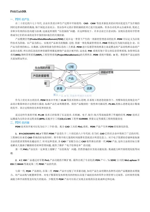
PMfiJSnMHR一、PDM的产生在二十世纪的六七十年代.企业在其设计和生产过程中开始使用,CAD、CAM等技术新技术的应用在促进生产为开展的同时也带来的新的挑战.始于制造企业而言,里站各单元的计算机辅助技术已是日技成熟,但各自动化单元自成体系,彼此之音林少有效的信息沟通与协调.这就是所谓的“信息抽防"问题。
在这种情况下,许多企业巳合意识到:实现信息的有序管理将成为它们的未来的竞争中保持依*地位的关饿因素.产品敷期甘理(ProductDataManaRemσnt,PDM)正是在这一背景下产生的一项新的管理思双的技术.PDM可以定义为以软件技术为茨础,以产品为核心,实现对产品相关的数据.过程.资源一体化集成管理技术.PIMI明南定位为面向前造全∙业,以产品为管理的核心,以数据.过程和资潦为管理信息的三大要素.PDM进行信愿管理的两条主故是整态的产品结构和动态的产品设计流程.所右的信息组织和资源管理都是困绕产品设计展开的.这也是PWi系统有别于其它的信息管理系境,如管理信息系统(MIS).物料管理系铳(MRP),工程管理系统(ProjectManaBeinen1.)的关然所在.PDM系统中数据:it程、费惹和产品这前的关臬如图1所示.生台周期侪理资题或管理产品.it卷.筑据和费源的关系图作为上世纪末出的技术,PDM继承并开展了C1.M等技术的核心思甥,在系统工程思怒的指导下,用整体优化的现念对产品设计数第和设计过程迸行描迹.标准产品生命周期普理,保持产品数招的一致性和可跟琮性.P1.M1.的核心思想是设计数端的有序、设计过程的优化和资界的扶里.是过近些年来的开展.P1.)M技术已经取得了长足进步,在机械、电子.航空/航天等故地荻俚了件遍的应用.PDM技术正运潮成为支持企业过程业组(BPR).实施并行工程(CE).C1.MS工程和S109000.贾量认迂等桑筑工程的使能技也二、PDM的开展PDM技术的开展可以化为以下三个阶∙段,配合CAD工具的PIn1.系统、PDM产品产生和PDM的琼准化阶段.1.B⅜CADXΛMPO∣M1.t早期的PDM产品设生于二十世纪的八十年代初.在当时.CAD巳羟在企业中得到了广泛的应用,工程婶们在承受CAD带来的好处的同时,势不得不将大量的时同泡费有查找设计所需信息上,对于电子筑堪的存储和荻取新方法的需求变得纯东越迫切了.针对这种需求,各CAD厂家配合自己CAD软件推出的第一代PDM产品,这些主品的目标主要是解决大量曲子翻狷的存府和管理问题,提供了维护“电子给国仓卑”的功能.第一代PM1.产品仅在一定和度上缓解了“信息孤岛’问题,仍然普遍存在至诜功能较弱。


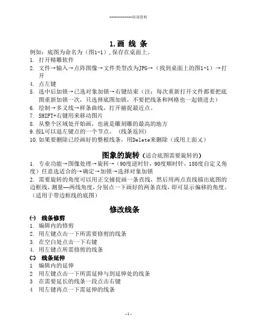
1.画线条例如:底图为命名为(图1-1),保存在桌面上。
1. 打开精雕软件2. 文件→输入→点阵图像→文件类型改为JPG→(找到桌面上的图1-1)→打开4. 点左键5. 选中后加锁→已选对象加锁→右键结束(注:每次重新打开文件都要把底图重新加锁一次,只选择底图加锁,不要把线条和网格也一起锁进去)6. 绘制→多义线→样条曲线,打开捕捉最近点。
7. SHIFT+右键用来移动图片8. 从整个区域处开始画,也就是雕刻雕的最高的地方9.按L可以退左键点的一个节点。
(线条返回)10.如果要删除已经画好的整根线条,用Delete来删除(或用上面乂)图象的旋转(适合底图需要旋转的)1.专业功能→图像处理→旋转→(90度逆时针,90度顺时针,180度自定义角度)任意选适合的→确定→加锁→选择对象加锁2.需要旋转的角度可以用正交捕捉画一条直线,然后用两点直线描出底图的边框线,测量—两线角度,分别点一下画好的两条直线,即可显示偏移的角度。
(适用于带边框线的底图)修改线条㈠线条修剪1. 编辑内的修剪2. 用左键点击一下所需要修剪的线条3. 在空白处点击一下右键4. 用左键点所需修剪的线条㈡线条延伸1 编辑内的延伸2 用左键点击一下所需延伸与到延伸处的线条3 在需要延长的线条一段点击右键4 用左键再点一下需延伸的线条㈢线条切断3选中线条→点编辑→切断→鼠标左键点一下所需要切断的地方连接功能1. 在左边→节点编辑工具(可以合并断点,重点等。
)线条的连接1. 点编辑→连接→点屏幕右边的缺省连接→用左键点击两条要连接的线条。
2. 对象为同一区域的两条直线可以连接2.建模型填颜色1. 虚拟雕塑工具→选中图片(把图片框起来)2. 模型→新建模型(把步长该为合适的)→右键确定3. 颜色→单线填色→选择一种颜色→点一下要填色的线条→按CTRL+左键(在填好颜色的线条里面画虚线(辅助填颜色用)1.画虚线→先选颜色上的单线填色→把单线填好→按空格键→再左键画线填色3.冲压→去料1. 选好填色后的图片2. 用雕塑→冲压→右边的颜色(外)→选底色【按Shift键鼠标左键点底色】→冲压深度(3-4毫米)3. 在模型里面扫一遍(按左键把黑的涂干净)→右键结束4. 选项→地图方式显示,(有颜色的图象=选项内的图形方式显示)5. 雕塑→去料→限高(冲压的高度)颜色模板(颜色内)6. 按Shift键把鼠标键放在自己要做的区内,选当前颜色7. Ctrl+右键是看立体的效果(旋转查看)8. 返回按鼠标右键选俯视图:冲压错误怎样返回1. 如果冲压错误了,再重新回到冲压→颜色无效冲压02. 如果去料错了要重新开始,雕塑→冲压→右边的颜色内→冲压深度(如3CM)→按住Shift键点击一下左键,松开Shift再点击一下左键,→右键结束;3. 如图在进了模型后跑掉图片→左边上的眼睛点一下;刀的区别H——对刀的显示与隐藏 Q——指刀的浅度E——线条显示与隐藏 W——指刀的深度N——取消颜色 A——指刀的直径放小R—模型显示与隐藏 S——指刀的直径放大G——颜色显示与隐藏 D——指刀的窄度Z——撤销一步 F——指刀的宽度限高保低如要做(4)毫米量:现有6毫米,应限高保低到选项→限高保低→限高填上→确定加载模型颜色(找回丢失的颜色)1. 必须是之前填的颜色是保存过的,而失去颜色后没有再次保存.2. 先把窗口缩小到下面的任务栏中3. 打开从前那幅有颜色的图片→模型→存为位图→保存(输入文件名)→右边确定→关掉这个窗口;4. 打开失去颜色图片的窗口→模型→加载模型颜色→打开刚才所保存的文件名三角刀导动——导动去料:1. 如果线条全部集合,先选中一条线条再按(Shift+左键)点完叶茎的线→导动去料→调好刀的深浅→右边颜色模板内→笔画类型选好→中间点一下;2. 导动方向不一样可以调整→变换→调整方向→右边的反向点一下磨光1. 效果→磨光→高度模式:任意选择(1) 去高补低,(2) 仅补低,(3) 仅补高,(4) 颜色模板(5) 磨光力度档任意选【一档慢(细)。

同望软件培训资料1. 简介同望软件是一家专业从事电力系统设计和仿真软件开发的公司,其产品包括PowerFactory、PowerStation等。
为了更好地服务客户,同望软件会不定期举办一些培训课程,为用户提供系统的学习和实践机会。
本文档梳理了同望软件培训资料的相关信息,包括培训内容、参与方式等。
2. 培训内容同望软件的培训课程主要涵盖以下几个方面:2.1. 电力系统基础知识此部分主要介绍电力系统的基础知识和理论,包括电网结构、电力传输和配电、设备的基本原理和参数等。
理解这些基础知识有助于更好地理解和使用同望软件的电力系统仿真软件。
2.2. PowerFactory软件使用PowerFactory是同望软件的一款电力系统仿真软件,培训课程将详细介绍其使用方法和技巧,包括数据输入、模型构建、分析和结果展示等各个环节。
参与者可以通过实际操作加深对软件的了解和理解。
2.3. PowerStation软件使用PowerStation是同望软件的一款电力系统设计软件,与PowerFactory相辅相成。
此部分主要介绍PowerStation的使用方法和技巧,包括基本的接线图绘制、电气设计、系统优化等内容。
3. 参与方式同望软件的培训课程可以通过以下几种方式参与:3.1. 线下培训课程同望软件会选择不同的城市和时间举办线下培训课程,参与者需提前报名并支付相应的培训费用。
线下培训课程通常包含理论讲解和实践操作环节,参与者可以通过和同行业人士的沟通和交流加深对电力系统和软件的理解。
3.2. 在线视频课程同望软件还提供在线视频课程,参与者可以自由选择时间和地点进行学习。
在线视频课程通常包括针对不同使用者的视频教程和相关的实践案例分析。
参与者可以根据自己的需要有选择地学习其中的内容。
3.3. 在线讲座同望软件还会定期开展一些在线讲座,以专题形式介绍相关的电力系统问题和解决方案。
参与者只需在线注册即可获得资格,并在指定时间收听线上讲座。
PDMS入门培训教程近年来,PDMS(Plant Design Management System)成为了化工、石油、天然气等行业的必备软件,它有着广泛的应用。
对于刚接触PDMS软件的初学者来说,入门培训非常重要,下面将为大家介绍一些PDMS入门培训教程。
一、基础知识首先,学习PDMS软件需要了解一些基础知识,比如:计算机基础、三维空间基础、CAD方面的知识等。
建议在电脑基础打好的情况下,可以先学习一些基础的CAD知识,比如如何使用绘图命令,如何绘制图形等,这样才能更好地理解PDMS 软件的使用方法。
二、软件安装将PDMS软件安装到电脑中非常重要,因为它是实际进行培训的软件。
如果没有软件,那么任何学习都是空谈。
PDMS 软件的安装步骤需要注意的是一些细节,如果安装不到位,那么会影响到软件的使用。
三、软件操作在掌握了基础知识和成功安装软件之后,学习软件操作就是非常重要的一步。
首先,需要熟悉基本的界面组成和操作方式,在PDMS软件中,包括了主界面、几何对象创造、属性定义、动态复查、层等等。
然后通过实践,慢慢掌握操作方法,例如:如何添加材料、直接利用列表窗口添加新对象、利用透视图观察3D模型等等。
四、绘图技巧PDMS软件中,关键是建立3D模型,以便实现物理模拟、可视化,以及最后的造型、投入生产等。
所以,熟练掌握绘图技巧比较重要,需要掌握各种绘图命令的用法,比如:绘制直线、弧线,制作圆、矩形等基本图形,绘制线路、开孔等等。
五、PDMS实战在掌握了以上内容之后,比较重要的一步就是实战。
建议通过模拟实际的场景,进行练习,加深理解。
比如:模拟制作一个压缩机的示意图,或者模拟制作一台车的立体模型,都是比较好的练习。
通过以上的步骤,初学者可以掌握PDMS软件的入门培训技巧,尽快熟练使用PDMS软件,学会PDMS软件的绘制方法,让自己在化工、石油等行业中有更好的发展。
当然,学习PDMS软件还需要不断实践和学习,只有耐心和精力才能取得好的成果。
CompuTherm Training ClassShanghai, ChinaNovember 15, 2007CompuTherm, LLCMadison, WI 53179, USACopyright © 2007 CompuTherm LLCCompuTherm Training Class, 2007CompuTherm Training Class, 200711.1 OptimizationThis material is intended for training users on how to use PanOptimizer with Al-Zn as an example. Understanding optimization process itself is more complicated and requires extensive experience.Users should follow the seven steps below to perform the model parameter optimization using PanOptimizer. Here we use Al-Zn binary as an example.9 Step 1: Load Thermodynamic Database FileLoad thermodynamic database AlZn_0.TDB file into Pandat workspace. This database file contains the phases to be modeled. The database file definition is consistent with the current accepted format in the CALPHAD society.9 Step 2: Define Model ParametersPanOptimizer asks user to define the optimization parameters in the TDB file. Each model parameter is defined by the keyword “OPTIMIZATION ”. The format of defining a model parameter is:Optimization [name of model parameter][low bound][initial value][high bound] N !For example:// Keyword Name Low Bound Init. Value High Bound Optimization LIQ_AA 0 0; 60000 N ! Optimization LIQ_AAT -20 0; 20 N !Phase LIQUID % 1 1 !Constituent LIQUID : AL, ZN : !Parameter G(LIQUID, AL; 0) 298.15 G_Al_LIQUID; 6000 N ! Parameter G(LIQUID, ZN; 0) 298.15 G_Zn_LIQUID; 6000 N ! Parameter G(LIQUID, AL, ZN; 0) 298.15 LIQ_AA + LIQ_AAT*T; 6000 N !9 Step 3: Prepare Experimental FileThe most widely accepted format for experimental data file in the CALPHAD society is a POP file. PanOptimizer accepts most of the keywords in the POP format and adds a few special keywords. Typical format of a POP file to define a tie line looks like:CREATE_NEW_EQUILIBRIUM 1,1 CHANGE_STATUS PHASE * = SCHANGE_STATUS PHASE LIQUID, FCC_A1 = FIX 1 SET_CONDITION P = P0, T = 656EXPERIMENT X(LIQUID, AL)= 0.33 : DX1, EXPERIMENT X(FCC_A1, AL)= 0.11 : DX1,CompuTherm Training Class, 2007 29 Step 4: Load and Compile Experimental FileThrough the function Load Experimental File , AlZn_Sample.pop file can be loaded into the Pandat workspace and compiled with the database file loaded in step 1.9 Step 5: OptimizationModel parameter optimization is controlled through the optimization control panel as shown below. There are four control areas in the optimization control panel. They are: Histogram (A), Bound/Unbound Variables (B), Optimization (C), and Optimization Results (D). Histogram (A)Histogram is for displaying and tracing the history of the discrepancy between model-calculated values and experimental data. Free Bound/Unbound Variables (B)The user can choose the model parameters to be optimized in either the bounded or the unbounded mode. In the bounded mode, the low and highbounds defined in a TDB file will take into effects.CompuTherm Training Class, 20073Optimization (C)The optimization process can be controlled by choosing 1 Iteration or Run . In this example, there are totally 11 parameters to be optimized and all the initial values are set to be zero. The available experimental data include the enthalpy of liquid phase at 953K, two invariant reactions at 655K: LIQUID -> FCC_A1 + HCP_A3 and at 550K: FCC_A1#2 -> FCC_A1#1 + HCP_A3 and tie-lines: FCC_A1#1 + FCC_A1#2, LIQUID + FCC_A1, LIQUID + HCP_A3 and HCP_A3 + FCC_A1 at different temperatures.Before the optimization, user can check the calculated results using the initial model parameters without optimization. The parameters without optimization result in large discrepancies between the calculated values and the experimental measurements. Optimization of these model parameters (value zero) is needed.AB C DCompuTherm Training Class, 20074By clicking Run twice (two rounds), and each Run with 50 number of function calls, the sum of squares decreases from 904896 to 494.After another two rounds of Run, the sum of squares decreases from 494 to 2.8. Now, we can do the real time calculation using the instantly obtained optimized parameters. The following two comparisons show excellent agreements between the calculated results and the measurement data.CompuTherm Training Class, 2007Optimization Results (D)•During optimization, user can check model parameters through the Parameters button.•For each model parameter, user can change its low bound, upper bound and initial value in the dialog window.•It also allows user to Include or Exclude some model parameters for optimization using “Ctrl” or “Shift” to select those parameters.•If a set of optimized parameters is satisfactory, user can save this set of values as default ones through Set As Default. Otherwise, user can reject this set of values and go back to previous default values through Reset Default.5CompuTherm Training Class, 2007 6• User also can save the TDB file with the optimized model parameters through Save TDB .• To track the change of each parameter during the past 100 iterations, user can click the parameter name in the table.•It should be noted that any changes on model parameters made by user will take into effect only after the “Apply” button is clicked.Comparison with Experimental Data (D)• Through Experimental Data , users can compare the calculated values and the experimental data for each equilibrium.• The experimental information such as uncertainty and weight factor can be adjusted as needed during optimization procedure.•Through the column of “Residual ”, user can see different color after each comparison. The green means satisfactory results are achieved, while the red color means large deviation remaining.• User can Include or Exclude the selected experimental data for the optimization as needed.• More detailed phase equilibrium information can be accessed by clicking the equilibrium ID in the table.•The “Export Table” function is used to export the table data to Excel.CompuTherm Training Class, 200779 Step 6: Plot Diagram with Pptimized ParametersDuring optimization, user can calculate phase equilibria or other properties at anytime using the instantly obtained optimized parameters, and plot the diagrams with experimental data. This provides a graphic presentation on the comparison between the calculated and experimental results. The parameters used for calculation are displayed in the Parameters window.CompuTherm Training Class, 200789 Step 7: Save/Load Optimization ResultsDuring optimization, the user may save and load optimization file through Save Optimization Results and Load Optimization Results . The optimization results file has the extension name of POR that can only be read by PanOptimizer. All settings of the optimization are stored and recovered through these two operations. Examples on the settings are: what model parameters used in the optimization, and their changes from previous step; what experimental data used in the optimization, and their weight and uncertainty; and comparisons between calculated results and experimental data.1.2 Rough Search“Rough Search ” is used to obtain a rough topology of a phase diagram based on the given experimental data. It might be useful for quickly guessing the initial values of the model parameters at the beginning stage of theoptimization procedure.9Step 1: Load Thermodynamic Database File (same asSection 1.1)9Step 2: Define Model Parameters (same as Section 1.1)9Step 3: Prepare Experimental FileKeyword CREATE_ROUGH_EQUILIBRIUM is used to define phase equilibrium for rough search. When create a rough equilibrium, the status of phases in equilibrium can only be FIXED. The keyword PHASE_POINT is used to define the calculation conditions. No experimental data are allowed to be optimized for multiple-phase equilibria. However, a special case is the single-phase equilibrium. The thermodynamic property data of the single-phase equilibrium can be used as experimental data to optimize the model parameters. Example is:$ Tieline between HCP_A3 and FCC_A1 at 500K$ 10 is the weight factor of this equilibriumCREATE_ROUGH_EQUILIBRIUM @@, 1, 10CHANGE_STATUS PHASE FCC_A1, HCP_A3 = FIX 1PHASE_POINT P = P0, T = 500PHASE_POINT X(FCC_A1, AL)= 0.92, X(HCP_A3, AL)= 0.01For a phase described by a sublattice model, the initial value of an element or species in a sublattice should be specified using SET_START_VALUE.9Step 4: Load and Compile Experimental FileThrough the function Load Experimental File, AlZn_Sample_rough.pop file can be loaded into the Pandat workspace and compiled with the database file loaded in step 1. The “Rough Search” button in toolbar will be activated automatically if there are rough equilibria loaded into PanOptimizer.9Step 5: Rough SearchAgain, there are four control areas in the control panel for rough search as shown below (only Area C is marked since the other three areas are the same as the normal optimization control panel).CRough Search (C)There are two types of built-in optimization algorithms for Rough Search and they are Global Search and Local Search, as shown in area C.•Global Search is to search a set of good initial values of the model parameters within the whole searching domain, the initial values defined in TDB file will be ignored.•Local Search leads to a quick convergence to an optimal solution based on the given initial values of model parameters.The user can set the maximum number of function calls for both algorithms.For example, 1000 function evaluations of Global search lead to the sum of squares of 2.91. The figure below shows the calculated phase boundaries after a global search with 1000 function evaluations. It can be seen that the optimized parameters give a very similar topology with the known Al-Zn phase diagram. By clicking Local Search , the sum of squares decrease from 2.91 to 0.059, which reproduces the phase diagram in better agreement with the experimental one as you can see below.Optimization Results (D)•Model parameters can be checked through Parameters .•Chemical potential differences between any two phases in equilibrium can be accessed by Experimental Data . They are reflected by the values in column “(Wtd. Residual)^2” as shown in the dialog window below.• The weight factor of the equilibrium can be adjusted as needed during optimization procedure.• Chemical potential values of each phase in equilibrium can be accessed by clicking the buttons in the first column.• The “Export Table ” function is used to export the table data to Excel.9Step 6: Go Back to Normal OptimizationOnce the phase diagram topology is obtained, user can append the AlZn_sample.pop, and go through Steps 5-7 to obtain an optimal set of model parameters which can best fit phase diagram and thermodynamic properties.。