No unbiased estimator of the variance of K-fold cross-validation

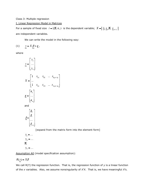
Class 3: Multiple regressionI. Linear Regression Model in Matrices For a sample of fixed size y n i,,1 is the dependent variable; 11,,1 p x x Xare independent variables. We can write the model in the following way:(1) X y ,wheren y y y (1))1()1(1211211...1......1p n p n n x x x x x x Xn (1)and110....p[expand from the matrix form into the element form]Assumption A0 (model specification assumption):X y R )(We call R(Y) the regression function. That is, the regression function of y is a linear function of the x variables. Also, we assume nonsingularity of X'X . That is, we have meaningful X 's..........21 n y y yII. Least Squares Estimator in Matrices Pre-multiply (1) by X ' (2),'''1 X X X y X pAssumption A1 (orthogonality assumption): we assume that is uncorrelated with each and every vector in X . That is,(3).0)(0),(0)(0),(0)(0),(0)(112111 p p x E x Cov x E x Cov x E x Cov ESample analog of expectation operator is n1. Thus, we have(4)01010101)1(21 i p i i i i i i x nx n x n n That is, there are a total of p restriction conditions, necessary for solving p linear equations to identify p parameters. In matrix format, this is equivalent to:(5).][or,][1o X o X nSubstitute (5) into (2), we have (6))()(X X y XThe LS estimator is then:(7),)(1y X X X bwhich is the same as the least squares estimator. Note: A1 assumption is needed for avoiding biases. III. Properties of the LS Estimator For the mode X y ,A1]using result, [important ][)(][)(])[(])[()]()[(])[()()(1111111o X E X X E X X X X X X X E X X X X E X X X X E y X X X E b E y X X X bthat is, b is unbiased.V (b ) is a symmetric matrix, called variance and covariance matrix of b .)(......)...(),(...),()()(1110100p b V b V b b Cov b b Cov b V b V 1111111)(][)()on al (condition ])[()])()[()]()[(])[()( X X X V X X X X X X X V O X X X X X X X V X X X X V y X X X V b V(after assuming I V 2][ non-serial correlation and homoscedasticity)21)( X X [important result, using A2][blackboard ]22001. Assumption A2 (iid assumption): independent and identically distributed errors. Two implications:1. Independent disturbances, j i E j i ,0),(Obtaining neat v (b ).2. Homoscedasticity, j i v E i j i ,)()(2Obtaining neat v (b ).I V 2)( , scalar matrix.IV. Fitted Values and Residualsy H y X X X X b X y 1)(ˆ X X X X H n n 1)(is called H matrix, or hat matrix. H is an idempotent matrix:H HHFor residuals:y H I y H y yy e )(ˆ (I-H ) is also an idempotent matrix.V. Estimation of the Residual Variance A. Sample Analog (8))()]([)(222i i i i E E E Vis unknown but can be estimated by e , where e is residual. Some of you may have noticedthat I have intentionally distinguished from e . is called disturbance, and e is called residual. Residual is defined by the difference between observed and predicted values.The sample analog of (8) is2)1()1(2211022)]([1)ˆ(11 p i p i i i i i i x b x b x b b y ny y n e nIn matrix:e e e i 2The sample analog is thenn e e /B. Degrees of FreedomAs a general rule, the correct degrees of freedom equals the number of totalobservations minus the number of parameters used in estimation.In multiple regression, there are p parameters to be estimated. Therefore, theremaining degrees of freedom for estimating disturbance variance is n-p . C. MSE as the EstimatorMSE is the unbiased estimator. It is unbiased because it corrects for the loss ofdegrees of freedom in estimating the parameters.ee p n MSE e pn MSE i112D. Statistical InferencesNow that we have point estimates (b ) and the variance-covariance matrix of b . But wecannot do formal statistical tests yet. The question, then, is how to make statistical inferences, such as testing hypotheses and constructing confidence intervals. Well, the only remaining thing we need is the ability to use some tests, say t , Z , or F tests.Statistical theory tells us that we can conduct such tests if e is not only iid, but iid in anormal distribution. That is, we assumeAssumption A3 (normality assumption): i is distributed as ),0(2NWith this assumption, we can look up tables for small samples.However, A3 is not necessary for large samples. For large samples, central limit theoryassures that we can still make the same statistical inferences based on t, z , or F tests if the sample is large enough.A Summary of Assumptions for the LS Estimator 1. A0: Specification assumptionX X y )|(EIncluding nonsingularity of X X .Meaningful X 's.With A0, we can computey X X X b 1)(2. A1:orthoganality assumption0)(k x E , for k = 0, .... p-1, x 0 = 1.Meaning: 0)( E is needed for the identification of 0 .All other column vectors in X are orthogonal with respect to .A1 is needed for avoiding biases. With A1, b is unbiased and consistent estimator of . Unbiasedness means that)(b EConsistency: n b as .For large samples, consistency is the most important criterion for evaluating estimators.3. A2. iid independent and identically distributed errors. Two implications:1. Independent disturbances, j i Cov j i ,0),(Obtaining neat v(b).2. Homoscedasticity, j i v Cov i j i ,)(),(2Obtaining neat v(b).I V 2)( , scalar matrix.With A2, b is an efficient estimator.Efficiency: an efficient estimator has the smallest sampling variance among all unbiased estimators. That is),ˆ()(Var somehow b Var whereˆ denotes any unbiased estimator. Roughly, for efficient estimators, imprecision [i.e., SD(b )] decreases by the inverse of the square root of n . That is, if you wish to increase precision by 10 times, (i.e., reduce S.E. by a factor of ten), you would need to increase the sample size by 100 times.A1 + A2 make OLS a BLUE estimator, where BLUE means the best, linear, unbiased estimator. That is, no other unbiased linear estimator has a smaller sampling variance than b .This result is called "Gauss-Markov theorem."4. A3. Normality, i is distributed as ),0(2NInferences: looking up tables for small samples.A1 + A2 + A3 make OLS a maximum likelihood (ML) estimator. Like all other ML estimators, OLS in this case is BUE (best unbiased estimator). That is, no other unbiased estimator can have a smaller sampling variance than OLS.Note that ML is always the most efficient estimator among all unbiased estimators. The cost of ML is really the requirement of we know the true parametric distribution of the residual. If you can afford the assumption, ML is always the best. Very often, we don't make the assumption because we don't know the parametric family of the disturbance. In general, the following tradeoff is true:More information == more efficiency. Less assumption == less efficiency.It is not correct to call certain models OLS models and other ML models. Theoretically, a same model can be estimated by OLS or ML. Model specification is different from estimation procedure.VI. ML for linear model under normality assumption (A1+A2+A3) , i :i :d N(0， 2), i = 1, … nObservations y i are independently distributed as y i ~ N(x i ’ 2); i = 1, … nUnder the normal errors assumption, the joint pdf of y’s isL = f (y 1…y n | 2) = ∏ f (y i | 2)= (2π 2)-n/2 exp{-(2 2)-1∑(y i - x i ’ }Log transformation is a monotone transformation. Maximizing L is equivalent to maximizing logL below:l = logL = (-n/2) log(2π 2) - (2 2)-1 ∑(y i - x i ’It is easy to see that what maximizes l (Maximum Likelihood Estimator) is the same as the LS estimator.。

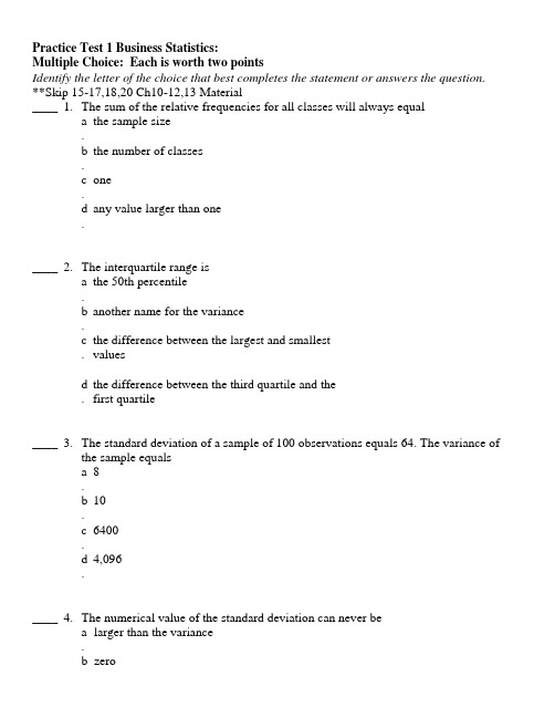
Practice Test 1 Business Statistics:Multiple Choice: Each is worth two pointsIdentify the letter of the choice that best completes the statement or answers the question. **Skip 15-17,18,20 Ch10-12,13 Material____ 1. The sum of the relative frequencies for all classes will always equal a.the sample sizeb.the number of classesc.oned.any value larger than one____ 2. The interquartile range isa.the 50th percentileb.another name for the variancec . the difference between the largest and smallest valuesd . the difference between the third quartile and the first quartile____ 3. The standard deviation of a sample of 100 observations equals 64. The variance of the sample equalsa.8b.10c.6400d.4,096____ 4. The numerical value of the standard deviation can never bea.larger than the variance.cnegative.smaller than the varianced.____ 5. The set of all possible sample points (experimental outcomes) is called aa sample.an eventb.cthe sample space.a populationd.____ 6. A random variable that can assume only a finite number of values is referred to as a(n)infinite sequencea.bfinite sequence.discrete random variablec.discrete probability functiond.Exhibit 5-11A local bottling company has determined the number of machine breakdowns permonth and their respective probabilities as shown below:Number ofBreakdowns Probability0 0.121 0.382 0.253 0.184 0.07____ 7. Refer to Exhibit 5-11. The probability of at least 3 breakdowns in a month is a0.5b0.10.c0.30.d0.90.____ 8. A normal probability distributionis a continuous probability distributiona.bis a discrete probability distribution.can be either continuous or discretec.dmust have a standard deviation of 1.Exhibit 6-6The starting salaries of individuals with an MBA degree are normally distributedwith a mean of $40,000 and a standard deviation of $5,000.____ 9. Refer to Exhibit 6-6. What percentage of MBA's will have starting salaries of $34,000 to $46,000?a38.49%.38.59%b.50%c.76.98%d.____10. Given that Z is a standard normal random variable, what is the value of Z if the area between -Z and Z is 0.901?1.96a.-1.96b.0.4505c.d 1.65____11. Which of the following is not a measure of central location?amean.medianb.variancec.moded.____12. The descriptive measure of dispersion that is based on the concept of a deviation about the mean isthe rangea.the interquartile rangeb.the absolute value of the rangec.the standard deviationd.____13. Which of the following symbols represents the mean of the population?aσ2.bσ.cμ.d.____14. Which of the following symbols represents the size of the sampleaσ2.bσ.Nc.d n____15. If two events are independent, thenathey must be mutually exclusive.the sum of their probabilities must be equal to oneb.ctheir intersection must be zero.None of these alternatives is correct..d.____16. Which of the following statements is(are) always true?a-1 ≤ P(E i) ≤1.P(A) = 1 - P(A c)b.P(A) + P(B) = 1c.d∑P ≥ 1.____17. A measure of the average value of a random variable is called a(n)variancea.bstandard deviation.expected valuec.coefficient of variationd.____18. Four percent of the customers of a mortgage company default on their payments. A sample of five customers is selected. What is the probability that exactly twocustomers in the sample will default on their payments?0.2592a.0.0142b..0.7408d.____19. The expected value of a discrete random variablea. is the most likely or highest probability value for the randomvariableb. will always be one of the values x can take on, although it maynot be the highest probability value for the random variablec. is the average value for the random variable over many repeats ofthe experimentd. None of these alternatives is correct.____20. Which of the following is not a property of a binomial experiment?a. the experiment consists of a sequence of n identical trialsb. each outcome can be referred to as a success or a failurec. the probabilities of the two outcomes can change from onetrial to the nextd. the trials are independentExhibit 5-9The probability distribution for the daily sales at Michael's Co. is given below.Daily Sales(In $1,000s) Probability40 0.150 0.460 0.370 0.2____21. Refer to Exhibit 5-9. The expected daily sales are$55,000a.$56,000b.$50,000c.$70,000d.azero.-0.5b.c0.5.oned.Exhibit 6-2The weight of football players is normally distributed with a mean of 200 poundsand a standard deviation of 25 pounds.____23. Refer to Exhibit 6-2. What percent of players weigh between 180 and 220 pounds?a. 28.81%b0.5762%.c. 0.281%57.62%d.Exhibit 6-6The starting salaries of individuals with an MBA degree are normally distributedwith a mean of $40,000 and a standard deviation of $5,000.____24. Refer to Exhibit 6-6. What is the probability that a randomly selected individual with an MBA degree will get a starting salary of at least $47,500?a. 0.4332b. 0.9332c. 0.0668d. 0.5000Short Answer/Problems1.The following data represent the daily demand (y in thousands of units) and the unit price (xin dollars) for a product.Daily Demand (y) Unit Price (x)47 139 335 544 334 620 815 16a. Compute and interpret the sample covariance for the above data.b. Compute and interpret the sample correlation coefficient.2.The daily dinner bills in a local restaurant are normally distributed with a mean of $28 and astandard deviation of $6.a. What is the probability that a randomly selected bill will be at least $39.10?b. What percentage of the bills will be less than $16.90?c. What are the minimum and maximum of the middle 95% of the bills?d. If twelve of one day's bills had a value of at least $43.06, how many bills didthe restaurant collect on that day?3.Below you are given a partial computer output based on a sample of 7 observations, relatingan independent variable (x) and a dependent variable (y).Predictor Coefficient StandardErrorConstant 24.112 8.376x -0.252 0.253Analysis of VarianceSOURCE SSRegression 196.893Error 94.822a. Develop the estimated regression line.b. If you are given that x = 50, find the estimate of y based on your regressionequation.c. Determine the coefficient of determination and interpret your answer. Solutions to MC1. C2. D3. D4. C5. C6. C7. D8. A9. D 10. D11. C 12. D 13. C 14. D 15. D 16. B 17. C 18. B19. C 20. C 21. B 22. C 23. D 24. C 25. C 26. A27. B 28. D 29. CSolutions to Short Answer1. ANS:a. -47 (rounded). Since the covariance is negative, it indicates a negativerelationship between x and y.b. -0.922. There is a strong negative relationship between x and y.2. ANS:a. 0.0322b. 0.0322d. 2,0003. ANS:a. = 24.112 + 0.816xb. If x = 50 then = 24.112 + 0.816x 24.1 + 0.82 ( 50 ) = 65.1c. 0.675 So there is a fairly strong positive relationship between x and y.Practice Test 2 Business Statistics:Multiple Choice: Each is worth two pointsIdentify the letter of the choice that best completes the statement or answers the question.____ 1. The sample statistic s is the point estimator ofa. μbσ.c.d.____ 2. A sample statistic is an unbiased estimator of the population parameter ifa. the expected value of the sample statistic is equal to zerob. the expected value of the sample statistic is equal to onec. the expected value of the sample statistic is equal to thepopulation parameterd. it is equal to zero____ 3. A property of a point estimator that occurs whenever larger sample sizes tend to provide point estimates closer to the population parameter is known asa. efficiencyb. unbiased samplingc. consistencyd. relative estimation____ 4. A random sample of 121 bottles of cologne showed an average content of 4 ounces.It is known that the standard deviation of the contents (i.e., of the population) is 0.22ounces. In this problem the 0.22 isa. a parameterb. a statisticd. the average content of colognes in the long run____ 5. A sample of 92 observations is taken from an infinite population. The sampling distribution of is approximatelya. normal because is always approximately normally distributedb. normal because the sample size is small in comparison to thepopulation sizec. normal because of the central limit theoremd. None of these alternatives is correct.____ 6. As the number of degrees of freedom for a t distribution increases, the difference between the t distribution and the standard normal distributiona. becomes largerb. becomes smallerc. stays the samed. None of these alternatives is correct.____ 7. From a population of 200 elements, a sample of 49 elements is selected. It is determined that the sample mean is 56 and the sample standard deviation is 14. Thestandard error of the mean isa. 3b. 2c. greater than 2d. less than 2____ 8. Which of the following is(are) point estimator(s)?a. σb. μc. sd. α____ 9. A population characteristic, such as a population mean, is calleda. a statistica parameterb.c. a sampledthe mean deviation.____10. The sample statistic, such as , s, or , that provides the point estimate of the population parameter is known asa. a point estimatorb. a parameterc. a population parameterd. a population statistic____11. The fact that the sampling distribution of sample means can be approximated by a normal probability distribution whenever the sample size is large is based on thea. central limit theoremb. fact that we have tables of areas for the normal distributionc. assumption that the population has a normal distributiond. None of these alternatives is correct.____12. Random samples of size 17 are taken from a population that has 200 elements, a mean of 36, and a standard deviation of 8. The mean and the standard deviation ofthe sampling distribution of the sample means area. 8.7 and 1.94b. 36 and 1.94c. 36 and 1.86d. 36 and 8____13. When constructing a confidence interval for the population mean and a small sample is used, the degrees of freedom for the t distribution equalsa. n-1b. nc. 29d. 30_____ 14. The collection of all possible sample points in an experiment isa. the sample spaceb. a sample pointc.an experimentd. the population_____ 15. Of five letters (A, B, C, D, and E), two letters are to be selected at random. How many possible selections are there?a. 20b. 7c. 5!d. 10_____ 16. The “Top Three” at a racetrack consists of picking the correct order of the first three horses in a race. If there are 10 horses in a particular race, how many “Top Three”outcomes are there?a. 302,400b. 720c. 1,814,400d. 10_____ 17. Given that event E has a probability of 0.25, the probability of the complement of event Ea. cannot be determined with the above informationb. can have any value between zero and onec. must be 0.75d. is 0.25_____ 18. The symbol ⋃ shows thea.union of eventsb. intersection of eventsc.sum of the probabilities of eventsd.sample space_____ 19. If P(A) = 0.38, P(B) = 0.83, and P(A ⋂ B) = 0.57; then P(A ⋃ B) =a. 1.21b. 0.64c. 0.78d. 1.78_____ 20. If P(A) = 0.62, P(B) = 0.47, and P(A ⋃ B) = 0.88; then P(A ⋂ B) =a. 0.2914b. 1.9700c. 0.6700d.0.2100_____ 21. If P(A) = 0.85, P(A ⋃ B) = 0.72, and P(A ⋂ B) = 0.66, then P(B) =a. 0.15b. 0.53c. 0.28d. 0.15_____ 22. Two events are mutually exclusive ifa. the probability of their intersection is 1b. they have no sample points in commonc. the probability of their intersection is 0.5d. the probability of their intersection is 1 and they have no sample points in common_____ 23. If A and B are mutually exclusive events with P(A) = 0.3 and P(B) = 0.5, then P(A ⋂ B) =a. 0.30b. 0.15c. 0.00d. 0.20_____ 24. If A and B are mutually exclusive events with P(A) = 0.3 and P(B) = 0.5, then P(A ⋃ B) =a. 0.00b. 0.15c. 0.8d. 0.2_____ 25. A subset of a population selected to represent the population is aa.subsetb.samplec.small populationd. None of the alternative answers is correct._____ 26. A simple random sample of size n from an infinite population of size N is to be selected. Each possible sample should havea. the same probability of being selectedb. a probability of 1/n of being selectedc. a probability of 1/N of being selectedd. a probability of N/n of being selected_____ 27. A probability distribution for all possible values of a sample statistic is known as aa.sample statisticb.parameterc.simple random sampled.sampling distribution_____ 28. From a population of 200 elements, the standard deviation is known to be 14.A sample of 49 elements is selected. It is determined that the sample mean is 56. The standard error of the mean isa. 3b. 2c. greater than 2d. less than 2_____ 29. From a population of 500 elements, a sample of 225 elements is selected. It is known that the variance of the population is 900. The standard error of the mean is approximatelya. 1.1022b. 2c. 30d. 1.4847Short Answer/ProblemsDirections: Clearly designate your solution to each portion of the questions asked and show your entire work and method for arriving at the solution.1. The sales records of a real estate agency show the following sales over the past 200 days:b. Assign probabilities to the sample points and show their values.c. What is the probability that the agency will not sell any houses in a given day?d. What is the probability of selling at least 2 houses?e. What is the probability of selling 1 or 2 houses?f. What is the probability of selling less than 3 houses?2. Assume two events A and B are mutually exclusive and, furthermore, P(A) = 0.2 and P(B)= 0.4.a. Find P(A ⋂ B).b. Find P(A ⋃ B).c. Find P(A⎜B).3.You are given the following information on Events A, B, C, and D. P(A) = .4, P(B) = .2,P(C) = .1,P(A ⋃ D) = .6, P(A⎜B) = .3, P(A ⋂ C) = .04, P(A ⋂ D) = .03a. Compute P(D).b. Compute P(A ⋂ B).c. Compute P(A⎜C).d. Compute the probability of the complement of C.e. Are A and B mutually exclusive? Explain your answer.f. Are A and B independent? Explain your answer.g. Are A and C mutually exclusive? Explain your answer.h. Are A and C independent? Explain your answer.4. Consider a population of five weights identical in appearance but weighing 1, 3, 5, 7, and 9 ounces.a. Determine the mean and the variance of the population.b. Sampling without replacement from the above population with a sample sizeof 2 produces ten possible samples. Using the ten sample mean values, determinethe mean of the population and the variance of .c. Compute the standard error of the mean.5. A population of 1,000 students spends an average of $10.50 a day on dinner. The standard deviation of the expenditure is $3. A simple random sample of 64 students is taken.a. What are the expected value, standard deviation, and shape of the samplingdistribution of the sample mean?b. What is the probability that these 64 students will spend a combined total of morethan $715.21?c. What is the probability that these 64 students will spend a combined total between$703.59 and $728.45?Solutions to MC Problems1. B 2 C 3. C 4. A 5. C 6. B 7. D 8. C 9. B 10. A11. A 12. C 13. A 14. A 15. D 16. B 17. C 18. A19. B 20. D 21. B 22. B 23. C 24. C 25. B 26. A27. D 28. D 29. DShort Answer/ProblemsDirections: Clearly designate your solution to each portion of the questions asked and show your entire work and method for arriving at the solution.1. ANSWERS:2. ANSWERS:a. 0.0 b. 0.6 c. 0.03ANSWERS:a. 0.23b. 0.06c. 0.4d. 0.9e. No, P(A⎜B) ≠ 0f. No, P(A⎜B) ≠ P(A)g. No, P(A ⋂ C) ≠ 0h. Yes, P(A⎜C) = P(A)4. ANSWERS:a. 5 and 8b. 5 and 3c. 1.7325. ANSWERS:a. 10.5 0.363 normalb. 0.0314c. 0.0794。

Class 5: ANOVA (Analysis of Variance) and F-testsI. What is ANOVAWhat is ANOVA? ANOVA is the short name for the Analysis of Variance. The essenceof ANOVA is to decompose the total variance of the dependent variable into two additive components, one for the structural part, and the other for the stochastic part, of a regression. Today we are going to examine the easiest case.II. ANOVA: An IntroductionLet the model beεβ+= X y .Assuming x i is a column vector (of length p) of independent variable values for the i th'observation,i i i εβ+='x y .Then b 'x i is the predicted value.sum of squares total:[]∑-=2Y y SST i []∑-+-=2'x b 'x y Y b i i i[][][][]∑∑∑-+-+-=Y -b 'x b 'x y 2Y b 'x b 'x y 22i i i i i i[][]∑∑-+=22Y b 'x e i ibecause [][][]∑∑=-=--0Y b 'x e Y b 'x b 'x y ii i i i .This is always true by OLS. = SSE + SSRImportant: the total variance of the dependent variable is decomposed into two additive parts: SSE, which is due to errors, and SSR, which is due to regression. Geometric interpretation: [blackboard ]Decomposition of VarianceIf we treat X as a random variable, we can decompose total variance to the between-group portion and the within-group portion in any population:()()()i i i x y εβV 'V V +=Prove:()()i i i x y εβ+='V V()()()i i i i x x εβεβ,'Cov 2V 'V ++=()()iix εβV 'V +=(by the assumption that ()0 ,'Cov =εβk x , for all possible k.)The ANOVA table is to estimate the three quantities of equation (1) from the sample.As the sample size gets larger and larger, the ANOVA table will approach the equation closer and closer.In a sample, decomposition of estimated variance is not strictly true. We thus need toseparately decompose sums of squares and degrees of freedom. Is ANOVA a misnomer?III. ANOVA in MatrixI will try to give a simplied representation of ANOVA as follows:[]∑-=2Y y SST i ()∑-+=i i y Y 2Y y 22∑∑∑-+=i i y Y 2Y y 22∑-+=222Y n 2Y n y i (because ∑=Y n y i )∑-=22Y n y i2Y n y 'y -=y J 'y n /1y 'y -= (in your textbook, monster look)SSE = e'e[]∑-=2Y b 'x SSR i()()[]∑-+=Y b 'x 2Y b 'x 22i i()[]()∑∑-+=b 'x Y 2Y n b 'x 22i i()[]()∑∑--+=i i i e y Y 2Y n b 'x 22()[]∑-+=222Y n 2Y n b 'x i(because ∑∑==0e ,Y n y i i , as always)()[]∑-=22Yn b 'x i2Y n Xb X'b'-=y J 'y n /1y X'b'-= (in your textbook, monster look)IV. ANOVA TableLet us use a real example. Assume that we have a regression estimated to be y = - 1.70 + 0.840 xANOVA TableSOURCE SS DF MS F with Regression 6.44 1 6.44 6.44/0.19=33.89 1, 18Error 3.40 18 0.19 Total 9.8419We know∑=100xi, ∑=50y i , 12.509x 2=∑i , 84.134y 2=∑i , ∑=66.257y x i i . If weknow that DF for SST=19, what is n?n= 205.220/50Y ==84.95.25.22084.134Y n y SST 22=⨯⨯-=-=∑i()[]∑-+=0.1250.84x 1.7-SSR 2i[]∑-⨯⨯⨯-⨯+⨯=0.125x 84.07.12x 84.084.07.17.12i i= 20⨯1.7⨯1.7+0.84⨯0.84⨯509.12-2⨯1.7⨯0.84⨯100- 125.0= 6.44SSE = SST-SSR=9.84-6.44=3.40DF (Degrees of freedom): demonstration. Note: discounting the intercept when calculating SST. MS = SS/DFp = 0.000 [ask students]. What does the p-value say?V. F-TestsF-tests are more general than t-tests, t-tests can be seen as a special case of F-tests.If you have difficulty with F-tests, please ask your GSIs to review F-tests in the lab. F-tests takes the form of a fraction of two MS's.MSR/MSE F , df2df1An F statistic has two degrees of freedom associated with it: the degree of freedom inthe numerator, and the degree of freedom in the denominator.An F statistic is usually larger than 1. The interpretation of an F statistics is thatwhether the explained variance by the alternative hypothesis is due to chance. In other words, the null hypothesis is that the explained variance is due to chance, or all the coefficients are zero.The larger an F-statistic, the more likely that the null hypothesis is not true. There is atable in the back of your book from which you can find exact probability values.In our example, the F is 34, which is highly significant.VI. R 2R 2 = SSR / SSTThe proportion of variance explained by the model. In our example, R-sq = 65.4%VII. What happens if we increase more independent variables.1. SST stays the same.2. SSR always increases.3. SSE always decreases.4. R 2 always increases.5. MSR usually increases.6. MSE usually decreases.7. F-test usually increases.Exceptions to 5 and 7: irrelevant variables may not explain the variance but take up degrees of freedom. We really need to look at the results.VIII. Important: General Ways of Hypothesis Testing with F-Statistics.All tests in linear regression can be performed with F-test statistics. The trick is to run"nested models."Two models are nested if the independent variables in one model are a subset or linearcombinations of a subset （子集）of the independent variables in the other model.That is to say. If model A has independent variables (1, 1x , 2x ), and model B hasindependent variables (1, 1x , 2x ,3x ), A and B are nested. A is called the restricted model; B is called less restricted or unrestricted model. We call A restricted because A implies that0=3β. This is a restriction.Another example: C has independent variable (1, 1x , 2x +3x ), D has (1, 2x +3x ). C and A are not nested.C and B are nested. One restriction in C: 32ββ=.C andD are nested. One restriction in D: 0=1β. D and A are not nested.D and B are nested: two restriction in D: 32ββ=; 0=1β.We can always test hypotheses implied in the restricted models. Steps: run tworegression for each hypothesis, one for the restricted model and one for the unrestrictedmodel. The SST should be the same across the two models. What is different is SSE and SSR. That is, what is different is R 2. Let()()df df SSE ,df df SSE u u r r ==;df df ()()0u r u r r u n p n p p p -=---=-<Use the following formulas:()()()()(),SSE SSE /df SSE df SSE F SSE /df r u r u dfr dfu dfu u u---=or()()()()(),SSR SSR /df SSR df SSR F SSE /df u r u r dfr dfu dfu u u---=(proof: use SST = SSE+SSR)Note, df(SSE r )-df(SSE u ) = df(SSR u )-df(SSR r ) =df ∆,is the number of constraints (not number of parameters) implied by the restricted modelor()()()22,2R R /df F 1R /dfur dfr dfu dfuuu--∆=- Note thatdf 1df ,2F t =That is, for 1df tests, you can either do an F-test or a t-test. They yield the same result. Another way to look at it is that the t-test is a special case of the F test, with the numerator DF being 1.IX. Assumptions of F-testsWhat assumptions do we need to make an ANOVA table work?Not much an assumption. All we need is the assumption that (X'X) is not singular, so that the least square estimate b exists.The assumption of ε'X =0 is needed if you want the ANOVA table to be an unbiased estimate of the true ANOVA (equation 1) in the population. Reason: we want b to be an unbiased estimator of β, and the covariance between b and εto disappear.For reasons I discussed earlier, the assumptions of homoscedasticity and non-serial correlation are necessary for the estimation of ()i V ε.The normality assumption that εi is distributed in a normal distribution is needed for small samples.X. The Concept of IncrementEvery time you put one more independent variable into your model, you get an increase in 2R . We sometime called the increase "incremental 2R ." What is means is that more variance is explained, or SSR is increased, SSE is reduced. What you should understand is that the incremental 2R attributed to a variable is always smaller than the 2R when other variables are absent.XI. Consequences of Omitting Relevant Independent VariablesSay the true model is the following:0112233i i i i i y x x x ββββε=++++.But for some reason we only collect or consider data on 21,,x and x y . Therefore, we omit3x in the regression. That is, we omit in 3x our model. We briefly discussed this problembefore. The short story is that we are likely to have a bias due to the omission of a relevant variable in the model. This is so even though our primary interest is to estimate the effect of1x or 2x on y.Why? We will have a formal presentation of this problem.XII. Measures of Goodness-of-FitThere are different ways to assess the goodness-of-fit of a model. A. R 2R 2 is a heuristic measure for the overall goodness-of-fit. It does not have an associated test statistic.R 2 measures the proportion of the variance in the dependent variable that is “explained” by the model: R 2 =SSESSR SSRSST SSR +=B. Model F-testThe model F-test tests the joint hypotheses that all the model coefficients except for the constant term are zero.Degrees of freedoms associated with the model F-test: Numerator: p-1 Denominator: n-p.C. t-tests for individual parametersA t-test for an individual parameter tests the hypothesis that a particular coefficient is equal to a particular number (commonly zero).t k = (b k - βk0)/SE k , where SE k is the (k, k) element of MSE(X’X)-1, with degree of freedom=n-p. D. Incremental R 2Relative to a restricted model, the gain in R 2 for the unrestricted model: ∆R 2= R u 2- R r 2E. F-tests for Nested ModelIt is the most general form of F-tests and t-tests.()()()()(),SSE SSE /df SSE df SSE F SSE /df r u r dfu dfr u dfu u u---=It is equal to a t-test if the unrestricted and restricted models differ only by one single parameter.It is equal to the model F-test if we set the restricted model to the constant-only model.[Ask students] What are SST, SSE, and SSR, and their associated degrees of freedom, for the constant-only model?Numerical ExampleA sociological study is interested in understanding the social determinants of mathematicalachievement among high school students. You are now asked to answer a series of questions. The data are real but have been tailored for educational purposes. The total number of observations is 400. The variables are defined as: y: math scorex1: father's education x2: mother's educationx3: family's socioeconomic status x4: number of siblings x5: class rankx6: parents' total education (note: x6 = x1 + x2) For the following regression models, we know: Table 1 SST SSR SSE DF R 2 (1) y on (1 x1 x2 x3 x4) 34863 4201 (2) y on (1 x6 x3 x4) 34863 396 .1065 (3) y on (1 x6 x3 x4 x5) 34863 10426 24437 395 .2991 (4) x5 on (1 x6 x3 x4) 269753 396 .02101. Please fill the missing cells in Table 1.2. Test the hypothesis that the effects of father's education (x1) and mother's education (x2) on math score are the same after controlling for x3 and x4.3. Test the hypothesis that x6, x3 and x4 in Model (2) all have a zero effect on y.4. Can we add x6 to Model (1)? Briefly explain your answer.5. Test the hypothesis that the effect of class rank (x5) on math score is zero after controlling for x6, x3, and x4.Answer: 1. SST SSR SSE DF R 2 (1) y on (1 x1 x2 x3 x4) 34863 4201 30662 395 .1205 (2) y on (1 x6 x3 x4) 34863 3713 31150 396 .1065 (3) y on (1 x6 x3 x4 x5) 34863 10426 24437 395 .2991 (4) x5 on (1 x6 x3 x4) 275539 5786 269753 396 .0210Note that the SST for Model (4) is different from those for Models (1) through (3). 2.Restricted model is 01123344()y b b x x b x b x e =+++++Unrestricted model is ''''''011223344y b b x b x b x b x e =+++++(31150 - 30662)/1F 1,395 = -------------------- = 488/77.63 = 6.29 30662 / 395 3.3713 / 3F 3,396 = --------------- = 1237.67 / 78.66 = 15.73 31150 / 3964. No. x6 is a linear combination of x1 and x2. X'X is singular.5.(31150 - 24437)/1F 1,395 = -------------------- = 6713 / 61.87 = 108.50 24437/395t = 10.42t ===。

S.-T.Yau College Student Mathematics Contests 2011Analysis and Differential EquationsIndividual2:30–5:00pm,July 9,2011(Please select 5problems to solve)1.a)Compute the integral: ∞−∞x cos xdx (x 2+1)(x 2+2),b)Show that there is a continuous function f :[0,+∞)→(−∞,+∞)such that f ≡0and f (4x )=f (2x )+f (x ).2.Solve the following problem: d 2u dx 2−u (x )=4e −x ,x ∈(0,1),u (0)=0,dudx(0)=0.3.Find an explicit conformal transformation of an open set U ={|z |>1}\(−∞,−1]to the unit disc.4.Assume f ∈C 2[a,b ]satisfying |f (x )|≤A,|f(x )|≤B for each x ∈[a,b ]and there exists x 0∈[a,b ]such that |f (x 0)|≤D ,then |f (x )|≤2√AB +D,∀x ∈[a,b ].5.Let C ([0,1])denote the Banach space of real valued continuous functions on [0,1]with the sup norm,and suppose that X ⊂C ([0,1])is a dense linear subspace.Suppose l :X →R is a linear map (not assumed to be continuous in any sense)such that l (f )≥0if f ∈X and f ≥0.Show that there is a unique Borel measure µon [0,1]such that l (f )= fdµfor all f ∈X .6.For s ≥0,let H s (T )be the space of L 2functions f on the circle T =R /(2πZ )whose Fourier coefficients ˆf n = 2π0e−inx f (x )dx satisfy Σ(1+n 2)s ||ˆf n |2<∞,with norm ||f ||2s =(2π)−1Σ(1+n 2)s |ˆf n |2.a.Show that for r >s ≥0,the inclusion map i :H r (T )→H s (T )is compact.b.Show that if s >1/2,then H s (T )includes continuously into C (T ),the space of continuous functions on T ,and the inclusion map is compact.1S.-T.Yau College Student Mathematics Contests2011Geometry and TopologyIndividual9:30–12:00am,July10,2011(Please select5problems to solve)1.Suppose M is a closed smooth n-manifold.a)Does there always exist a smooth map f:M→S n from M into the n-sphere,such that f is essential(i.e.f is not homotopic to a constant map)?Justify your answer.b)Same question,replacing S n by the n-torus T n.2.Suppose(X,d)is a compact metric space and f:X→X is a map so that d(f(x),f(y))=d(x,y)for all x,y in X.Show that f is an onto map.3.Let C1,C2be two linked circles in R3.Show that C1cannot be homotopic to a point in R3\C2.4.Let M=R2/Z2be the two dimensional torus,L the line3x=7y in R2,and S=π(L)⊂M whereπ:R2→M is the projection map. Find a differential form on M which represents the Poincar´e dual of S.5.A regular curve C in R3is called a Bertrand Curve,if there existsa diffeomorphism f:C→D from C onto a different regular curve D in R3such that N x C=N f(x)D for any x∈C.Here N x C denotes the principal normal line of the curve C passing through x,and T x C will denote the tangent line of C at x.Prove that:a)The distance|x−f(x)|is constant for x∈C;and the angle made between the directions of the two tangent lines T x C and T f(x)D is also constant.b)If the curvature k and torsionτof C are nowhere zero,then there must be constantsλandµsuch thatλk+µτ=16.Let M be the closed surface generated by carrying a small circle with radius r around a closed curve C embedded in R3such that the center moves along C and the circle is in the normal plane to C at each point.Prove thatMH2dσ≥2π2,and the equality holds if and only if C is a circle with radius √2r.HereH is the mean curvature of M and dσis the area element of M.1S.-T.Yau College Student Mathematics Contests 2011Algebra,Number Theory andCombinatoricsIndividual2:30–5:00pm,July 10,2011(Please select 5problems to solve)For the following problems,every example and statement must be backed up by proof.Examples and statements without proof will re-ceive no-credit.1.Let K =Q (√−3),an imaginary quadratic field.(a)Does there exists a finite Galois extension L/Q which containsK such that Gal(L/Q )∼=S 3?(Here S 3is the symmetric group in 3letters.)(b)Does there exists a finite Galois extension L/Q which containsK such that Gal(L/Q )∼=Z /4Z ?(c)Does there exists a finite Galois extension L/Q which containsK such that Gal(L/Q )∼=Q ?Here Q is the quaternion group with 8elements {±1,±i,±j,±k },a finite subgroup of the group of units H ×of the ring H of all Hamiltonian quaternions.2.Let f be a two-dimensional (complex)representation of a finite group G such that 1is an eigenvalue of f (σ)for every σ∈G .Prove that f is a direct sum of two one-dimensional representations of G3.Let F ⊂R be the subset of all real numbers that are roots of monic polynomials f (X )∈Q [X ].(1)Show that F is a field.(2)Show that the only field automorphisms of F are the identityautomorphism α(x )=x for all x ∈F .4.Let V be a finite-dimensional vector space over R and T :V →V be a linear transformation such that(1)the minimal polynomial of T is irreducible;(2)there exists a vector v ∈V such that {T i v |i ≥0}spans V .Show that V contains no non-trivial proper T -invariant subspace.5.Given a commutative diagramA →B →C →D →E↓↓↓↓↓A →B →C →D →E1Algebra,Number Theory and Combinatorics,2011-Individual2 of Abelian groups,such that(i)both rows are exact sequences and(ii) every vertical map,except the middle one,is an isomorphism.Show that the middle map C→C is also an isomorphism.6.Prove that a group of order150is not simple.S.-T.Yau College Student Mathematics Contests 2011Applied Math.,Computational Math.,Probability and StatisticsIndividual6:30–9:00pm,July 9,2011(Please select 5problems to solve)1.Given a weight function ρ(x )>0,let the inner-product correspond-ing to ρ(x )be defined as follows:(f,g ):= baρ(x )f (x )g (x )d x,and let f :=(f,f ).(1)Define a sequence of polynomials as follows:p 0(x )=1,p 1(x )=x −a 1,p n (x )=(x −a n )p n −1(x )−b n p n −2(x ),n =2,3,···wherea n =(xp n −1,p n −1)(p n −1,p n −1),n =1,2,···b n =(xp n −1,p n −2)(p n −2,p n −2),n =2,3,···.Show that {p n (x )}is an orthogonal sequence of monic polyno-mials.(2)Let {q n (x )}be an orthogonal sequence of monic polynomialscorresponding to the ρinner product.(A polynomial is called monic if its leading coefficient is 1.)Show that {q n (x )}is unique and it minimizes q n amongst all monic polynomials of degree n .(3)Hence or otherwise,show that if ρ(x )=1/√1−x 2and [a,b ]=[−1,1],then the corresponding orthogonal sequence is the Cheby-shev polynomials:T n (x )=cos(n arccos x ),n =0,1,2,···.and the following recurrent formula holds:T n +1(x )=2xT n (x )−T n −1(x ),n =1,2,···.(4)Find the best quadratic approximation to f (x )=x 3on [−1,1]using ρ(x )=1/√1−x 2.1Applied Math.Prob.Stat.,2011-Individual 22.If two polynomials p (x )and q (x ),both of fifth degree,satisfyp (i )=q (i )=1i,i =2,3,4,5,6,andp (1)=1,q (1)=2,find p (0)−q (0)y aside m black balls and n red balls in a jug.Supposes 1≤r ≤k ≤n .Each time one draws a ball from the jug at random.1)If each time one draws a ball without return,what is the prob-ability that in the k -th time of drawing one obtains exactly the r -th red ball?2)If each time one draws a ball with return,what is the probability that in the first k times of drawings one obtained totally an odd number of red balls?4.Let X and Y be independent and identically distributed random variables.Show thatE [|X +Y |]≥E [|X |].Hint:Consider separately two cases:E [X +]≥E [X −]and E [X +]<E [X −].5.Suppose that X 1,···,X n are a random sample from the Bernoulli distribution with probability of success p 1and Y 1,···,Y n be an inde-pendent random sample from the Bernoulli distribution with probabil-ity of success p 2.(a)Give a minimum sufficient statistic and the UMVU (uniformlyminimum variance unbiased)estimator for θ=p 1−p 2.(b)Give the Cramer-Rao bound for the variance of the unbiasedestimators for v (p 1)=p 1(1−p 1)or the UMVU estimator for v (p 1).(c)Compute the asymptotic power of the test with critical region |√n (ˆp 1−ˆp 2)/ 2ˆp ˆq |≥z 1−αwhen p 1=p and p 2=p +n −1/2∆,where ˆp =0.5ˆp 1+0.5ˆp 2.6.Suppose that an experiment is conducted to measure a constant θ.Independent unbiased measurements y of θcan be made with either of two instruments,both of which measure with normal errors:fori =1,2,instrument i produces independent errors with a N (0,σ2i )distribution.The two error variances σ21and σ22are known.When ameasurement y is made,a record is kept of the instrument used so that after n measurements the data is (a 1,y 1),...,(a n ,y n ),where a m =i if y m is obtained using instrument i .The choice between instruments is made independently for each observation in such a way thatP (a m =1)=P (a m =2)=0.5,1≤m ≤n.Applied Math.Prob.Stat.,2011-Individual 3Let x denote the entire set of data available to the statistician,in this case (a 1,y 1),...,(a n ,y n ),and let l θ(x )denote the corresponding log likelihood function for θ.Let a =n m =1(2−a m ).(a)Show that the maximum likelihood estimate of θis given by ˆθ= n m =11/σ2a m −1 n m =1y m /σ2a m.(b)Express the expected Fisher information I θand the observedFisher information I x in terms of n ,σ21,σ22,and a .What hap-pens to the quantity I θ/I x as n →∞?(c)Show that a is an ancillary statistic,and that the conditional variance of ˆθgiven a equals 1/I x .Of the two approximations ˆθ·∼N (θ,1/I θ)and ˆθ·∼N (θ,1/I x ),which (if either)would you use for the purposes of inference,and why?S.-T.Yau College Student Mathematics Contests 2011Analysis and Differential EquationsTeam9:00–12:00am,July 9,2011(Please select 5problems to solve)1.Let H 2(∆)be the space of holomorphic functions in the unit disk ∆={|z |<1}such that ∆|f |2|dz |2<∞.Prove that H 2(∆)is a Hilbert space and that for any r <1,the map T :H 2(∆)→H 2(∆)given by T f (z ):=f (rz )is a compact operator.2.For any continuous function f (z )of period 1,show that the equation dϕdt=2πϕ+f (t )has a unique solution of period 1.3.Let h (x )be a C ∞function on the real line R .Find a C ∞function u (x,y )on an open subset of R containing the x -axis such that u x +2u y =u 2and u (x,0)=h (x ).4.Let S ={x ∈R ||x −p |≤c/q 3,for all p,q ∈Z ,q >0,c >0},show that S is uncountable and its measure is zero.5.Let sl (n )denote the set of all n ×n real matrices with trace equal to zero and let SL (n )be the set of all n ×n real matrices with deter-minant equal to one.Let ϕ(z )be a real analytic function defined in a neighborhood of z =0of the complex plane C satisfying the conditions ϕ(0)=1and ϕ (0)=1.(a)If ϕmaps any near zero matrix in sl (n )into SL (n )for some n ≥3,show that ϕ(z )=exp(z ).(b)Is the conclusion of (a)still true in the case n =2?If it is true,prove it.If not,give a counterexample.e mathematical analysis to show that:(a)e and πare irrational numbers;(b)e and πare also transcendental numbers.1S.-T.Yau College Student Mathematics Contests2011Applied Math.,Computational Math.,Probability and StatisticsTeam9:00–12:00am,July9,2011(Please select5problems to solve)1.Let A be an N-by-N symmetric positive definite matrix.The con-jugate gradient method can be described as follows:r0=b−A x0,p0=r0,x0=0FOR n=0,1,...αn= r n 22/(p TnA p n)x n+1=x n+αn p n r n+1=r n−αn A p nβn=−r Tk+1A p k/p TkA p kp n+1=r n+1+βn p nEND FORShow(a)αn minimizes f(x n+αp n)for allα∈R wheref(x)≡12x T A x−b T x.(b)p Ti r n=0for i<n and p TiA p j=0if i=j.(c)Span{p0,p1,...,p n−1}=Span{r0,r1,...,r n−1}≡K n.(d)r n is orthogonal to K n.2.We use the following scheme to solve the PDE u t+u x=0:u n+1 j =au nj−2+bu nj−1+cu njwhere a,b,c are constants which may depend on the CFL numberλ=∆t ∆x .Here x j=j∆x,t n=n∆t and u njis the numerical approximationto the exact solution u(x j,t n),with periodic boundary conditions.(i)Find a,b,c so that the scheme is second order accurate.(ii)Verify that the scheme you derived in Part(i)is exact(i.e.u nj =u(x j,t n))ifλ=1orλ=2.Does this imply that the scheme is stable forλ≤2?If not,findλ0such that the scheme is stable forλ≤λ0. Recall that a scheme is stable if there exist constants M and C,which are independent of the mesh sizes∆x and∆t,such thatu n ≤Me CT u0for all∆x,∆t and n such that t n≤T.You can use either the L∞norm or the L2norm to prove stability.1Applied Math.Prob.Stat.,2011-Team2 3.Let X and Y be independent random variables,identically dis-tributed according to the Normal distribution with mean0and variance 1,N(0,1).(a)Find the joint probability density function of(R,),whereR=(X2+Y2)1/2andθ=arctan(Y/X).(b)Are R andθindependent?Why,or why not?(c)Find a function U of R which has the uniform distribution on(0,1),Unif(0,1).(d)Find a function V ofθwhich is distributed as Unif(0,1).(e)Show how to transform two independent observations U and Vfrom Unif(0,1)into two independent observations X,Y fromN(0,1).4.Let X be a random variable such that E[|X|]<∞.Show thatE[|X−a|]=infE[|X−x|],x∈Rif and only if a is a median of X.5.Let Y1,...,Y n be iid observations from the distribution f(x−θ), whereθis unknown and f()is probability density function symmetric about zero.Suppose a priori thatθhas the improper priorθ∼Lebesgue(flat) on(−∞,∞).Write down the posterior distribution ofθ.Provides some arguments to show that thisflat prior is noninforma-tive.Show that with the posterior distribution in(a),a95%probability interval is also a95%confidence interval.6.Suppose we have two independent random samples{Y1,i=1,...,n} from Poisson with(unknown)meanλ1and{Y i,i=n+1,...,2n}from Poisson with(unknown)meanλ2Letθ=λ1/(λ1+λ2).(a)Find an unbiased estimator ofθ(b)Does your estimator have the minimum variance among all un-biased estimators?If yes,prove it.If not,find one that has theminimum variance(and prove it).(c)Does the unbiased minimum variance estimator you found at-tain the Fisher information bound?If yes,show it.If no,whynot?S.-T.Yau College Student Mathematics Contests2011Geometry and TopologyTeam9:00–12:00am,July9,2011(Please select5problems to solve)1.Suppose K is afinite connected simplicial complex.True or false:a)Ifπ1(K)isfinite,then the universal cover of K is compact.b)If the universal cover of K is compact thenπ1(K)isfinite.pute all homology groups of the the m-skeleton of an n-simplex, 0≤m≤n.3.Let M be an n-dimensional compact oriented Riemannian manifold with boundary and X a smooth vectorfield on M.If n is the inward unit normal vector of the boundary,show thatM div(X)dV M=∂MX·n dV∂M.4.Let F k(M)be the space of all C∞k-forms on a differentiable man-ifold M.Suppose U and V are open subsets of M.a)Explain carefully how the usual exact sequence0−→F(U∪V)−→F(U)⊕F V)−→F(U∩V)−→0 arises.b)Write down the“long exact sequence”in de Rham cohomology as-sociated to the short exact sequence in part(a)and describe explicitly how the mapH kdeR (U∩V)−→H k+1deR(U∪V)arises.5.Let M be a Riemannian n-manifold.Show that the scalar curvature R(p)at p∈M is given byR(p)=1vol(S n−1)S n−1Ric p(x)dS n−1,where Ric p(x)is the Ricci curvature in direction x∈S n−1⊂T p M, vol(S n−1)is the volume of S n−1and dS n−1is the volume element of S n−1.1Geometry and Topology,2011-Team2 6.Prove the Schur’s Lemma:If on a Riemannian manifold of dimension at least three,the Ricci curvature depends only on the base point but not on the tangent direction,then the Ricci curvature must be constant everywhere,i.e.,the manifold is Einstein.S.-T.Yau College Student Mathematics Contests 2011Algebra,Number Theory andCombinatoricsTeam9:00–12:00pm,July 9,2011(Please select 5problems to solve)For the following problems,every example and statement must be backed up by proof.Examples and statements without proof will re-ceive no-credit.1.Let F be a field and ¯Fthe algebraic closure of F .Let f (x,y )and g (x,y )be polynomials in F [x,y ]such that g .c .d .(f,g )=1in F [x,y ].Show that there are only finitely many (a,b )∈¯F×2such that f (a,b )=g (a,b )=0.Can you generalize this to the cases of more than two-variables?2.Let D be a PID,and D n the free module of rank n over D .Then any submodule of D n is a free module of rank m ≤n .3.Identify pairs of integers n =m ∈Z +such that the quotient rings Z [x,y ]/(x 2−y n )∼=Z [x,y ]/(x 2−y m );and identify pairs of integers n =m ∈Z +such that Z [x,y ]/(x 2−y n )∼=Z [x,y ]/(x 2−y m ).4.Is it possible to find an integer n >1such that the sum1+12+13+14+ (1)is an integer?5.Recall that F 7is the finite field with 7elements,and GL 3(F 7)is the group of all invertible 3×3matrices with entries in F 7.(a)Find a 7-Sylow subgroup P 7of GL 3(F 7).(b)Determine the normalizer subgroup N of the 7-Sylow subgroupyou found in (a).(c)Find a 2-Sylow subgroup of GL 3(F 7).6.For a ring R ,let SL 2(R )denote the group of invertible 2×2matrices.Show that SL 2(Z )is generated by T = 1101 and S = 01−10 .What about SL 2(R )?1。

ls定理 umvueUMVUE（Uniformly Minimum Variance Unbiased Estimator）是指在所有无偏估计量中方差最小的估计量。

UMVUE是统计学中一个重要的概念，它具有很高的实用性和理论价值。

本文将围绕UMVUE展开讨论，介绍其定义、特性以及在实际问题中的应用。

一、UMVUE的定义UMVUE是指在所有无偏估计量中方差最小的估计量。

为了更好地理解UMVUE的概念，我们先来了解一下无偏估计量的定义。

无偏估计量是指估计量的期望值等于被估计参数的真实值。

无偏估计量的定义表明其在大样本情况下具有较好的性质，但并不保证方差最小。

而UMVUE则在所有无偏估计量中选取方差最小的作为估计量，使得估计结果更加精确和可靠。

二、UMVUE的特性UMVUE具有以下几个重要的特性：1. UMVUE是无偏估计量：UMVUE的定义要求其是无偏估计量，即其期望值等于被估计参数的真实值。

2. UMVUE是唯一的：在一定条件下，UMVUE是唯一的，即不存在其他无偏估计量的方差更小。

3. UMVUE的方差最小：UMVUE是所有无偏估计量中方差最小的估计量，因此具有较好的精确性和可靠性。

4. UMVUE的有效性：UMVUE在大样本情况下具有较好的有效性，即方差较小。

三、UMVUE的应用UMVUE在实际问题中有着广泛的应用，下面我们将介绍一些常见的应用场景。

1. 参数估计：UMVUE常用于对参数的估计，例如正态分布的均值和方差的估计等。

在参数估计中，UMVUE可以提供较为准确的估计结果。

2. 假设检验：UMVUE在假设检验中也有重要的应用。

例如，利用UMVUE可以进行对总体均值、总体方差等参数的假设检验。

3. 回归分析：在回归分析中，UMVUE可以用于对回归系数的估计。

通过选择UMVUE作为估计量，可以使得回归模型的拟合效果更好。

4. 变量选择：UMVUE还可以用于变量选择。

在变量选择中，通过选择UMVUE可以排除掉冗余的变量，提高模型的解释能力。

T his appendix derives various results for ordinary least squares estimation of themultiple linear regression model using matrix notation and matrix algebra (see Appendix D for a summary). The material presented here is much more ad-vanced than that in the text.E.1THE MODEL AND ORDINARY LEAST SQUARES ESTIMATIONThroughout this appendix,we use the t subscript to index observations and an n to denote the sample size. It is useful to write the multiple linear regression model with k parameters as follows:y t ϭ␤1ϩ␤2x t 2ϩ␤3x t 3ϩ… ϩ␤k x tk ϩu t ,t ϭ 1,2,…,n ,(E.1)where y t is the dependent variable for observation t ,and x tj ,j ϭ 2,3,…,k ,are the inde-pendent variables. Notice how our labeling convention here differs from the text:we call the intercept ␤1and let ␤2,…,␤k denote the slope parameters. This relabeling is not important,but it simplifies the matrix approach to multiple regression.For each t ,define a 1 ϫk vector,x t ϭ(1,x t 2,…,x tk ),and let ␤ϭ(␤1,␤2,…,␤k )Јbe the k ϫ1 vector of all parameters. Then,we can write (E.1) asy t ϭx t ␤ϩu t ,t ϭ 1,2,…,n .(E.2)[Some authors prefer to define x t as a column vector,in which case,x t is replaced with x t Јin (E.2). Mathematically,it makes more sense to define it as a row vector.] We can write (E.2) in full matrix notation by appropriately defining data vectors and matrices. Let y denote the n ϫ1 vector of observations on y :the t th element of y is y t .Let X be the n ϫk vector of observations on the explanatory variables. In other words,the t th row of X consists of the vector x t . Equivalently,the (t ,j )th element of X is simply x tj :755A p p e n d i x EThe Linear Regression Model inMatrix Formn X ϫ k ϵϭ .Finally,let u be the n ϫ 1 vector of unobservable disturbances. Then,we can write (E.2)for all n observations in matrix notation :y ϭX ␤ϩu .(E.3)Remember,because X is n ϫ k and ␤is k ϫ 1,X ␤is n ϫ 1.Estimation of ␤proceeds by minimizing the sum of squared residuals,as in Section3.2. Define the sum of squared residuals function for any possible k ϫ 1 parameter vec-tor b asSSR(b ) ϵ͚nt ϭ1(y t Ϫx t b )2.The k ϫ 1 vector of ordinary least squares estimates,␤ˆϭ(␤ˆ1,␤ˆ2,…,␤ˆk )؅,minimizes SSR(b ) over all possible k ϫ 1 vectors b . This is a problem in multivariable calculus.For ␤ˆto minimize the sum of squared residuals,it must solve the first order conditionѨSSR(␤ˆ)/Ѩb ϵ0.(E.4)Using the fact that the derivative of (y t Ϫx t b )2with respect to b is the 1ϫ k vector Ϫ2(y t Ϫx t b )x t ,(E.4) is equivalent to͚nt ϭ1xt Ј(y t Ϫx t ␤ˆ) ϵ0.(E.5)(We have divided by Ϫ2 and taken the transpose.) We can write this first order condi-tion as͚nt ϭ1(y t Ϫ␤ˆ1Ϫ␤ˆ2x t 2Ϫ… Ϫ␤ˆk x tk ) ϭ0͚nt ϭ1x t 2(y t Ϫ␤ˆ1Ϫ␤ˆ2x t 2Ϫ… Ϫ␤ˆk x tk ) ϭ0...͚nt ϭ1x tk (y t Ϫ␤ˆ1Ϫ␤ˆ2x t 2Ϫ… Ϫ␤ˆk x tk ) ϭ0,which,apart from the different labeling convention,is identical to the first order condi-tions in equation (3.13). We want to write these in matrix form to make them more use-ful. Using the formula for partitioned multiplication in Appendix D,we see that (E.5)is equivalent to΅1x 12x 13...x 1k1x 22x 23...x 2k...1x n 2x n 3...x nk ΄΅x 1x 2...x n ΄Appendix E The Linear Regression Model in Matrix Form756Appendix E The Linear Regression Model in Matrix FormXЈ(yϪX␤ˆ) ϭ0(E.6) or(XЈX)␤ˆϭXЈy.(E.7)It can be shown that (E.7) always has at least one solution. Multiple solutions do not help us,as we are looking for a unique set of OLS estimates given our data set. Assuming that the kϫ k symmetric matrix XЈX is nonsingular,we can premultiply both sides of (E.7) by (XЈX)Ϫ1to solve for the OLS estimator ␤ˆ:␤ˆϭ(XЈX)Ϫ1XЈy.(E.8)This is the critical formula for matrix analysis of the multiple linear regression model. The assumption that XЈX is invertible is equivalent to the assumption that rank(X) ϭk, which means that the columns of X must be linearly independent. This is the matrix ver-sion of MLR.4 in Chapter 3.Before we continue,(E.8) warrants a word of warning. It is tempting to simplify the formula for ␤ˆas follows:␤ˆϭ(XЈX)Ϫ1XЈyϭXϪ1(XЈ)Ϫ1XЈyϭXϪ1y.The flaw in this reasoning is that X is usually not a square matrix,and so it cannot be inverted. In other words,we cannot write (XЈX)Ϫ1ϭXϪ1(XЈ)Ϫ1unless nϭk,a case that virtually never arises in practice.The nϫ 1 vectors of OLS fitted values and residuals are given byyˆϭX␤ˆ,uˆϭyϪyˆϭyϪX␤ˆ.From (E.6) and the definition of uˆ,we can see that the first order condition for ␤ˆis the same asXЈuˆϭ0.(E.9) Because the first column of X consists entirely of ones,(E.9) implies that the OLS residuals always sum to zero when an intercept is included in the equation and that the sample covariance between each independent variable and the OLS residuals is zero. (We discussed both of these properties in Chapter 3.)The sum of squared residuals can be written asSSR ϭ͚n tϭ1uˆt2ϭuˆЈuˆϭ(yϪX␤ˆ)Ј(yϪX␤ˆ).(E.10)All of the algebraic properties from Chapter 3 can be derived using matrix algebra. For example,we can show that the total sum of squares is equal to the explained sum of squares plus the sum of squared residuals [see (3.27)]. The use of matrices does not pro-vide a simpler proof than summation notation,so we do not provide another derivation.757The matrix approach to multiple regression can be used as the basis for a geometri-cal interpretation of regression. This involves mathematical concepts that are even more advanced than those we covered in Appendix D. [See Goldberger (1991) or Greene (1997).]E.2FINITE SAMPLE PROPERTIES OF OLSDeriving the expected value and variance of the OLS estimator ␤ˆis facilitated by matrix algebra,but we must show some care in stating the assumptions.A S S U M P T I O N E.1(L I N E A R I N P A R A M E T E R S)The model can be written as in (E.3), where y is an observed nϫ 1 vector, X is an nϫ k observed matrix, and u is an nϫ 1 vector of unobserved errors or disturbances.A S S U M P T I O N E.2(Z E R O C O N D I T I O N A L M E A N)Conditional on the entire matrix X, each error ut has zero mean: E(ut͉X) ϭ0, tϭ1,2,…,n.In vector form,E(u͉X) ϭ0.(E.11) This assumption is implied by MLR.3 under the random sampling assumption,MLR.2.In time series applications,Assumption E.2 imposes strict exogeneity on the explana-tory variables,something discussed at length in Chapter 10. This rules out explanatory variables whose future values are correlated with ut; in particular,it eliminates laggeddependent variables. Under Assumption E.2,we can condition on the xtjwhen we com-pute the expected value of ␤ˆ.A S S U M P T I O N E.3(N O P E R F E C T C O L L I N E A R I T Y) The matrix X has rank k.This is a careful statement of the assumption that rules out linear dependencies among the explanatory variables. Under Assumption E.3,XЈX is nonsingular,and so ␤ˆis unique and can be written as in (E.8).T H E O R E M E.1(U N B I A S E D N E S S O F O L S)Under Assumptions E.1, E.2, and E.3, the OLS estimator ␤ˆis unbiased for ␤.P R O O F:Use Assumptions E.1 and E.3 and simple algebra to write␤ˆϭ(XЈX)Ϫ1XЈyϭ(XЈX)Ϫ1XЈ(X␤ϩu)ϭ(XЈX)Ϫ1(XЈX)␤ϩ(XЈX)Ϫ1XЈuϭ␤ϩ(XЈX)Ϫ1XЈu,(E.12)where we use the fact that (XЈX)Ϫ1(XЈX) ϭIk . Taking the expectation conditional on X givesAppendix E The Linear Regression Model in Matrix Form 758E(␤ˆ͉X)ϭ␤ϩ(XЈX)Ϫ1XЈE(u͉X)ϭ␤ϩ(XЈX)Ϫ1XЈ0ϭ␤,because E(u͉X) ϭ0under Assumption E.2. This argument clearly does not depend on the value of ␤, so we have shown that ␤ˆis unbiased.To obtain the simplest form of the variance-covariance matrix of ␤ˆ,we impose the assumptions of homoskedasticity and no serial correlation.A S S U M P T I O N E.4(H O M O S K E D A S T I C I T Y A N DN O S E R I A L C O R R E L A T I O N)(i) Var(ut͉X) ϭ␴2, t ϭ 1,2,…,n. (ii) Cov(u t,u s͉X) ϭ0, for all t s. In matrix form, we canwrite these two assumptions asVar(u͉X) ϭ␴2I n,(E.13)where Inis the nϫ n identity matrix.Part (i) of Assumption E.4 is the homoskedasticity assumption:the variance of utcan-not depend on any element of X,and the variance must be constant across observations, t. Part (ii) is the no serial correlation assumption:the errors cannot be correlated across observations. Under random sampling,and in any other cross-sectional sampling schemes with independent observations,part (ii) of Assumption E.4 automatically holds. For time series applications,part (ii) rules out correlation in the errors over time (both conditional on X and unconditionally).Because of (E.13),we often say that u has scalar variance-covariance matrix when Assumption E.4 holds. We can now derive the variance-covariance matrix of the OLS estimator.T H E O R E M E.2(V A R I A N C E-C O V A R I A N C EM A T R I X O F T H E O L S E S T I M A T O R)Under Assumptions E.1 through E.4,Var(␤ˆ͉X) ϭ␴2(XЈX)Ϫ1.(E.14)P R O O F:From the last formula in equation (E.12), we haveVar(␤ˆ͉X) ϭVar[(XЈX)Ϫ1XЈu͉X] ϭ(XЈX)Ϫ1XЈ[Var(u͉X)]X(XЈX)Ϫ1.Now, we use Assumption E.4 to getVar(␤ˆ͉X)ϭ(XЈX)Ϫ1XЈ(␴2I n)X(XЈX)Ϫ1ϭ␴2(XЈX)Ϫ1XЈX(XЈX)Ϫ1ϭ␴2(XЈX)Ϫ1.Appendix E The Linear Regression Model in Matrix Form759Formula (E.14) means that the variance of ␤ˆj (conditional on X ) is obtained by multi-plying ␴2by the j th diagonal element of (X ЈX )Ϫ1. For the slope coefficients,we gave an interpretable formula in equation (3.51). Equation (E.14) also tells us how to obtain the covariance between any two OLS estimates:multiply ␴2by the appropriate off diago-nal element of (X ЈX )Ϫ1. In Chapter 4,we showed how to avoid explicitly finding covariances for obtaining confidence intervals and hypotheses tests by appropriately rewriting the model.The Gauss-Markov Theorem,in its full generality,can be proven.T H E O R E M E .3 (G A U S S -M A R K O V T H E O R E M )Under Assumptions E.1 through E.4, ␤ˆis the best linear unbiased estimator.P R O O F :Any other linear estimator of ␤can be written as␤˜ ϭA Јy ,(E.15)where A is an n ϫ k matrix. In order for ␤˜to be unbiased conditional on X , A can consist of nonrandom numbers and functions of X . (For example, A cannot be a function of y .) To see what further restrictions on A are needed, write␤˜ϭA Ј(X ␤ϩu ) ϭ(A ЈX )␤ϩA Јu .(E.16)Then,E(␤˜͉X )ϭA ЈX ␤ϩE(A Јu ͉X )ϭA ЈX ␤ϩA ЈE(u ͉X ) since A is a function of XϭA ЈX ␤since E(u ͉X ) ϭ0.For ␤˜to be an unbiased estimator of ␤, it must be true that E(␤˜͉X ) ϭ␤for all k ϫ 1 vec-tors ␤, that is,A ЈX ␤ϭ␤for all k ϫ 1 vectors ␤.(E.17)Because A ЈX is a k ϫ k matrix, (E.17) holds if and only if A ЈX ϭI k . Equations (E.15) and (E.17) characterize the class of linear, unbiased estimators for ␤.Next, from (E.16), we haveVar(␤˜͉X ) ϭA Ј[Var(u ͉X )]A ϭ␴2A ЈA ,by Assumption E.4. Therefore,Var(␤˜͉X ) ϪVar(␤ˆ͉X )ϭ␴2[A ЈA Ϫ(X ЈX )Ϫ1]ϭ␴2[A ЈA ϪA ЈX (X ЈX )Ϫ1X ЈA ] because A ЈX ϭI kϭ␴2A Ј[I n ϪX (X ЈX )Ϫ1X Ј]Aϵ␴2A ЈMA ,where M ϵI n ϪX (X ЈX )Ϫ1X Ј. Because M is symmetric and idempotent, A ЈMA is positive semi-definite for any n ϫ k matrix A . This establishes that the OLS estimator ␤ˆis BLUE. How Appendix E The Linear Regression Model in Matrix Form 760Appendix E The Linear Regression Model in Matrix Formis this significant? Let c be any kϫ 1 vector and consider the linear combination cЈ␤ϭc1␤1ϩc2␤2ϩ… ϩc k␤k, which is a scalar. The unbiased estimators of cЈ␤are cЈ␤ˆand cЈ␤˜. ButVar(c␤˜͉X) ϪVar(cЈ␤ˆ͉X) ϭcЈ[Var(␤˜͉X) ϪVar(␤ˆ͉X)]cՆ0,because [Var(␤˜͉X) ϪVar(␤ˆ͉X)] is p.s.d. Therefore, when it is used for estimating any linear combination of ␤, OLS yields the smallest variance. In particular, Var(␤ˆj͉X) ՅVar(␤˜j͉X) for any other linear, unbiased estimator of ␤j.The unbiased estimator of the error variance ␴2can be written as␴ˆ2ϭuˆЈuˆ/(n Ϫk),where we have labeled the explanatory variables so that there are k total parameters, including the intercept.T H E O R E M E.4(U N B I A S E D N E S S O F␴ˆ2)Under Assumptions E.1 through E.4, ␴ˆ2is unbiased for ␴2: E(␴ˆ2͉X) ϭ␴2for all ␴2Ͼ0. P R O O F:Write uˆϭyϪX␤ˆϭyϪX(XЈX)Ϫ1XЈyϭM yϭM u, where MϭI nϪX(XЈX)Ϫ1XЈ,and the last equality follows because MXϭ0. Because M is symmetric and idempotent,uˆЈuˆϭuЈMЈM uϭuЈM u.Because uЈM u is a scalar, it equals its trace. Therefore,ϭE(uЈM u͉X)ϭE[tr(uЈM u)͉X] ϭE[tr(M uuЈ)͉X]ϭtr[E(M uuЈ|X)] ϭtr[M E(uuЈ|X)]ϭtr(M␴2I n) ϭ␴2tr(M) ϭ␴2(nϪ k).The last equality follows from tr(M) ϭtr(I) Ϫtr[X(XЈX)Ϫ1XЈ] ϭnϪtr[(XЈX)Ϫ1XЈX] ϭnϪn) ϭnϪk. Therefore,tr(IkE(␴ˆ2͉X) ϭE(uЈM u͉X)/(nϪ k) ϭ␴2.E.3STATISTICAL INFERENCEWhen we add the final classical linear model assumption,␤ˆhas a multivariate normal distribution,which leads to the t and F distributions for the standard test statistics cov-ered in Chapter 4.A S S U M P T I O N E.5(N O R M A L I T Y O F E R R O R S)are independent and identically distributed as Normal(0,␴2). Conditional on X, the utEquivalently, u given X is distributed as multivariate normal with mean zero and variance-covariance matrix ␴2I n: u~ Normal(0,␴2I n).761Appendix E The Linear Regression Model in Matrix Form Under Assumption E.5,each uis independent of the explanatory variables for all t. Inta time series setting,this is essentially the strict exogeneity assumption.T H E O R E M E.5(N O R M A L I T Y O F␤ˆ)Under the classical linear model Assumptions E.1 through E.5, ␤ˆconditional on X is dis-tributed as multivariate normal with mean ␤and variance-covariance matrix ␴2(XЈX)Ϫ1.Theorem E.5 is the basis for statistical inference involving ␤. In fact,along with the properties of the chi-square,t,and F distributions that we summarized in Appendix D, we can use Theorem E.5 to establish that t statistics have a t distribution under Assumptions E.1 through E.5 (under the null hypothesis) and likewise for F statistics. We illustrate with a proof for the t statistics.T H E O R E M E.6Under Assumptions E.1 through E.5,(␤ˆjϪ␤j)/se(␤ˆj) ~ t nϪk,j ϭ 1,2,…,k.P R O O F:The proof requires several steps; the following statements are initially conditional on X. First, by Theorem E.5, (␤ˆjϪ␤j)/sd(␤ˆ) ~ Normal(0,1), where sd(␤ˆj) ϭ␴͙ෆc jj, and c jj is the j th diagonal element of (XЈX)Ϫ1. Next, under Assumptions E.1 through E.5, conditional on X,(n Ϫ k)␴ˆ2/␴2~ ␹2nϪk.(E.18)This follows because (nϪk)␴ˆ2/␴2ϭ(u/␴)ЈM(u/␴), where M is the nϫn symmetric, idem-potent matrix defined in Theorem E.4. But u/␴~ Normal(0,I n) by Assumption E.5. It follows from Property 1 for the chi-square distribution in Appendix D that (u/␴)ЈM(u/␴) ~ ␹2nϪk (because M has rank nϪk).We also need to show that ␤ˆand ␴ˆ2are independent. But ␤ˆϭ␤ϩ(XЈX)Ϫ1XЈu, and ␴ˆ2ϭuЈM u/(nϪk). Now, [(XЈX)Ϫ1XЈ]Mϭ0because XЈMϭ0. It follows, from Property 5 of the multivariate normal distribution in Appendix D, that ␤ˆand M u are independent. Since ␴ˆ2is a function of M u, ␤ˆand ␴ˆ2are also independent.Finally, we can write(␤ˆjϪ␤j)/se(␤ˆj) ϭ[(␤ˆjϪ␤j)/sd(␤ˆj)]/(␴ˆ2/␴2)1/2,which is the ratio of a standard normal random variable and the square root of a ␹2nϪk/(nϪk) random variable. We just showed that these are independent, and so, by def-inition of a t random variable, (␤ˆjϪ␤j)/se(␤ˆj) has the t nϪk distribution. Because this distri-bution does not depend on X, it is the unconditional distribution of (␤ˆjϪ␤j)/se(␤ˆj) as well.From this theorem,we can plug in any hypothesized value for ␤j and use the t statistic for testing hypotheses,as usual.Under Assumptions E.1 through E.5,we can compute what is known as the Cramer-Rao lower bound for the variance-covariance matrix of unbiased estimators of ␤(again762conditional on X ) [see Greene (1997,Chapter 4)]. This can be shown to be ␴2(X ЈX )Ϫ1,which is exactly the variance-covariance matrix of the OLS estimator. This implies that ␤ˆis the minimum variance unbiased estimator of ␤(conditional on X ):Var(␤˜͉X ) ϪVar(␤ˆ͉X ) is positive semi-definite for any other unbiased estimator ␤˜; we no longer have to restrict our attention to estimators linear in y .It is easy to show that the OLS estimator is in fact the maximum likelihood estima-tor of ␤under Assumption E.5. For each t ,the distribution of y t given X is Normal(x t ␤,␴2). Because the y t are independent conditional on X ,the likelihood func-tion for the sample is obtained from the product of the densities:͟nt ϭ1(2␲␴2)Ϫ1/2exp[Ϫ(y t Ϫx t ␤)2/(2␴2)].Maximizing this function with respect to ␤and ␴2is the same as maximizing its nat-ural logarithm:͚nt ϭ1[Ϫ(1/2)log(2␲␴2) Ϫ(yt Ϫx t ␤)2/(2␴2)].For obtaining ␤ˆ,this is the same as minimizing͚nt ϭ1(y t Ϫx t ␤)2—the division by 2␴2does not affect the optimization—which is just the problem that OLS solves. The esti-mator of ␴2that we have used,SSR/(n Ϫk ),turns out not to be the MLE of ␴2; the MLE is SSR/n ,which is a biased estimator. Because the unbiased estimator of ␴2results in t and F statistics with exact t and F distributions under the null,it is always used instead of the MLE.SUMMARYThis appendix has provided a brief discussion of the linear regression model using matrix notation. This material is included for more advanced classes that use matrix algebra,but it is not needed to read the text. In effect,this appendix proves some of the results that we either stated without proof,proved only in special cases,or proved through a more cumbersome method of proof. Other topics—such as asymptotic prop-erties,instrumental variables estimation,and panel data models—can be given concise treatments using matrices. Advanced texts in econometrics,including Davidson and MacKinnon (1993),Greene (1997),and Wooldridge (1999),can be consulted for details.KEY TERMSAppendix E The Linear Regression Model in Matrix Form 763First Order Condition Matrix Notation Minimum Variance Unbiased Scalar Variance-Covariance MatrixVariance-Covariance Matrix of the OLS EstimatorPROBLEMSE.1Let x t be the 1ϫ k vector of explanatory variables for observation t . Show that the OLS estimator ␤ˆcan be written as␤ˆϭΘ͚n tϭ1xt Јx t ΙϪ1Θ͚nt ϭ1xt Јy t Ι.Dividing each summation by n shows that ␤ˆis a function of sample averages.E.2Let ␤ˆbe the k ϫ 1 vector of OLS estimates.(i)Show that for any k ϫ 1 vector b ,we can write the sum of squaredresiduals asSSR(b ) ϭu ˆЈu ˆϩ(␤ˆϪb )ЈX ЈX (␤ˆϪb ).[Hint :Write (y Ϫ X b )Ј(y ϪX b ) ϭ[u ˆϩX (␤ˆϪb )]Ј[u ˆϩX (␤ˆϪb )]and use the fact that X Јu ˆϭ0.](ii)Explain how the expression for SSR(b ) in part (i) proves that ␤ˆuniquely minimizes SSR(b ) over all possible values of b ,assuming Xhas rank k .E.3Let ␤ˆbe the OLS estimate from the regression of y on X . Let A be a k ϫ k non-singular matrix and define z t ϵx t A ,t ϭ 1,…,n . Therefore,z t is 1ϫ k and is a non-singular linear combination of x t . Let Z be the n ϫ k matrix with rows z t . Let ␤˜denote the OLS estimate from a regression ofy on Z .(i)Show that ␤˜ϭA Ϫ1␤ˆ.(ii)Let y ˆt be the fitted values from the original regression and let y ˜t be thefitted values from regressing y on Z . Show that y ˜t ϭy ˆt ,for all t ϭ1,2,…,n . How do the residuals from the two regressions compare?(iii)Show that the estimated variance matrix for ␤˜is ␴ˆ2A Ϫ1(X ЈX )Ϫ1A Ϫ1؅,where ␴ˆ2is the usual variance estimate from regressing y on X .(iv)Let the ␤ˆj be the OLS estimates from regressing y t on 1,x t 2,…,x tk ,andlet the ␤˜j be the OLS estimates from the regression of yt on 1,a 2x t 2,…,a k x tk ,where a j 0,j ϭ 2,…,k . Use the results from part (i)to find the relationship between the ␤˜j and the ␤ˆj .(v)Assuming the setup of part (iv),use part (iii) to show that se(␤˜j ) ϭse(␤ˆj )/͉a j ͉.(vi)Assuming the setup of part (iv),show that the absolute values of the tstatistics for ␤˜j and ␤ˆj are identical.Appendix E The Linear Regression Model in Matrix Form 764。

计量经济学术语A校正R2（Adjusted R-Squared）：多元回归分析中拟合优度的量度，在估计误差的方差时对添加的解释变量用一个自由度来调整。

对立假设（Alternative Hypothesis）：检验虚拟假设时的相对假设。

AR（1）序列相关（AR(1) Serial Correlation）：时间序列回归模型中的误差遵循AR（1）模型。

渐近置信区间（Asymptotic Confidence Interval）：大样本容量下近似成立的置信区间。

渐近正态性（Asymptotic Normality）：适当正态化后样本分布收敛到标准正态分布的估计量。

渐近性质（Asymptotic Properties）：当样本容量无限增长时适用的估计量和检验统计量性质。

渐近标准误（Asymptotic Standard Error）：大样本下生效的标准误。

渐近t 统计量（Asymptotic t Statistic）：大样本下近似服从标准正态分布的t 统计量。

渐近方差（Asymptotic Variance）：为了获得渐近标准正态分布，我们必须用以除估计量的平方值。

渐近有效（Asymptotically Efficient）：对于服从渐近正态分布的一致性估计量，有最小渐近方差的估计量。

渐近不相关（Asymptotically Uncorrelated）：时间序列过程中，随着两个时点上的随机变量的时间间隔增加，它们之间的相关趋于零。

衰减偏误（Attenuation Bias）：总是朝向零的估计量偏误，因而有衰减偏误的估计量的期望值小于参数的绝对值。

自回归条件异方差性（Autoregressive Conditional Heteroskedasticity, ARCH）：动态异方差性模型，即给定过去信息，误差项的方差线性依赖于过去的误差的平方。

一阶自回归过程[AR（1）]（Autoregressive Process of Order One [AR(1)]）：一个时间序列模型，其当前值线性依赖于最近的值加上一个无法预测的扰动。

T his appendix derives various results for ordinary least squares estimation of themultiple linear regression model using matrix notation and matrix algebra (see Appendix D for a summary). The material presented here is much more ad-vanced than that in the text.E.1THE MODEL AND ORDINARY LEAST SQUARES ESTIMATIONThroughout this appendix,we use the t subscript to index observations and an n to denote the sample size. It is useful to write the multiple linear regression model with k parameters as follows:y t ϭ␤1ϩ␤2x t 2ϩ␤3x t 3ϩ… ϩ␤k x tk ϩu t ,t ϭ 1,2,…,n ,(E.1)where y t is the dependent variable for observation t ,and x tj ,j ϭ 2,3,…,k ,are the inde-pendent variables. Notice how our labeling convention here differs from the text:we call the intercept ␤1and let ␤2,…,␤k denote the slope parameters. This relabeling is not important,but it simplifies the matrix approach to multiple regression.For each t ,define a 1 ϫk vector,x t ϭ(1,x t 2,…,x tk ),and let ␤ϭ(␤1,␤2,…,␤k )Јbe the k ϫ1 vector of all parameters. Then,we can write (E.1) asy t ϭx t ␤ϩu t ,t ϭ 1,2,…,n .(E.2)[Some authors prefer to define x t as a column vector,in which case,x t is replaced with x t Јin (E.2). Mathematically,it makes more sense to define it as a row vector.] We can write (E.2) in full matrix notation by appropriately defining data vectors and matrices. Let y denote the n ϫ1 vector of observations on y :the t th element of y is y t .Let X be the n ϫk vector of observations on the explanatory variables. In other words,the t th row of X consists of the vector x t . Equivalently,the (t ,j )th element of X is simply x tj :755A p p e n d i x EThe Linear Regression Model inMatrix Formn X ϫ k ϵϭ .Finally,let u be the n ϫ 1 vector of unobservable disturbances. Then,we can write (E.2)for all n observations in matrix notation :y ϭX ␤ϩu .(E.3)Remember,because X is n ϫ k and ␤is k ϫ 1,X ␤is n ϫ 1.Estimation of ␤proceeds by minimizing the sum of squared residuals,as in Section3.2. Define the sum of squared residuals function for any possible k ϫ 1 parameter vec-tor b asSSR(b ) ϵ͚nt ϭ1(y t Ϫx t b )2.The k ϫ 1 vector of ordinary least squares estimates,␤ˆϭ(␤ˆ1,␤ˆ2,…,␤ˆk )؅,minimizes SSR(b ) over all possible k ϫ 1 vectors b . This is a problem in multivariable calculus.For ␤ˆto minimize the sum of squared residuals,it must solve the first order conditionѨSSR(␤ˆ)/Ѩb ϵ0.(E.4)Using the fact that the derivative of (y t Ϫx t b )2with respect to b is the 1ϫ k vector Ϫ2(y t Ϫx t b )x t ,(E.4) is equivalent to͚nt ϭ1xt Ј(y t Ϫx t ␤ˆ) ϵ0.(E.5)(We have divided by Ϫ2 and taken the transpose.) We can write this first order condi-tion as͚nt ϭ1(y t Ϫ␤ˆ1Ϫ␤ˆ2x t 2Ϫ… Ϫ␤ˆk x tk ) ϭ0͚nt ϭ1x t 2(y t Ϫ␤ˆ1Ϫ␤ˆ2x t 2Ϫ… Ϫ␤ˆk x tk ) ϭ0...͚nt ϭ1x tk (y t Ϫ␤ˆ1Ϫ␤ˆ2x t 2Ϫ… Ϫ␤ˆk x tk ) ϭ0,which,apart from the different labeling convention,is identical to the first order condi-tions in equation (3.13). We want to write these in matrix form to make them more use-ful. Using the formula for partitioned multiplication in Appendix D,we see that (E.5)is equivalent to΅1x 12x 13...x 1k1x 22x 23...x 2k...1x n 2x n 3...x nk ΄΅x 1x 2...x n ΄Appendix E The Linear Regression Model in Matrix Form756Appendix E The Linear Regression Model in Matrix FormXЈ(yϪX␤ˆ) ϭ0(E.6) or(XЈX)␤ˆϭXЈy.(E.7)It can be shown that (E.7) always has at least one solution. Multiple solutions do not help us,as we are looking for a unique set of OLS estimates given our data set. Assuming that the kϫ k symmetric matrix XЈX is nonsingular,we can premultiply both sides of (E.7) by (XЈX)Ϫ1to solve for the OLS estimator ␤ˆ:␤ˆϭ(XЈX)Ϫ1XЈy.(E.8)This is the critical formula for matrix analysis of the multiple linear regression model. The assumption that XЈX is invertible is equivalent to the assumption that rank(X) ϭk, which means that the columns of X must be linearly independent. This is the matrix ver-sion of MLR.4 in Chapter 3.Before we continue,(E.8) warrants a word of warning. It is tempting to simplify the formula for ␤ˆas follows:␤ˆϭ(XЈX)Ϫ1XЈyϭXϪ1(XЈ)Ϫ1XЈyϭXϪ1y.The flaw in this reasoning is that X is usually not a square matrix,and so it cannot be inverted. In other words,we cannot write (XЈX)Ϫ1ϭXϪ1(XЈ)Ϫ1unless nϭk,a case that virtually never arises in practice.The nϫ 1 vectors of OLS fitted values and residuals are given byyˆϭX␤ˆ,uˆϭyϪyˆϭyϪX␤ˆ.From (E.6) and the definition of uˆ,we can see that the first order condition for ␤ˆis the same asXЈuˆϭ0.(E.9) Because the first column of X consists entirely of ones,(E.9) implies that the OLS residuals always sum to zero when an intercept is included in the equation and that the sample covariance between each independent variable and the OLS residuals is zero. (We discussed both of these properties in Chapter 3.)The sum of squared residuals can be written asSSR ϭ͚n tϭ1uˆt2ϭuˆЈuˆϭ(yϪX␤ˆ)Ј(yϪX␤ˆ).(E.10)All of the algebraic properties from Chapter 3 can be derived using matrix algebra. For example,we can show that the total sum of squares is equal to the explained sum of squares plus the sum of squared residuals [see (3.27)]. The use of matrices does not pro-vide a simpler proof than summation notation,so we do not provide another derivation.757The matrix approach to multiple regression can be used as the basis for a geometri-cal interpretation of regression. This involves mathematical concepts that are even more advanced than those we covered in Appendix D. [See Goldberger (1991) or Greene (1997).]E.2FINITE SAMPLE PROPERTIES OF OLSDeriving the expected value and variance of the OLS estimator ␤ˆis facilitated by matrix algebra,but we must show some care in stating the assumptions.A S S U M P T I O N E.1(L I N E A R I N P A R A M E T E R S)The model can be written as in (E.3), where y is an observed nϫ 1 vector, X is an nϫ k observed matrix, and u is an nϫ 1 vector of unobserved errors or disturbances.A S S U M P T I O N E.2(Z E R O C O N D I T I O N A L M E A N)Conditional on the entire matrix X, each error ut has zero mean: E(ut͉X) ϭ0, tϭ1,2,…,n.In vector form,E(u͉X) ϭ0.(E.11) This assumption is implied by MLR.3 under the random sampling assumption,MLR.2.In time series applications,Assumption E.2 imposes strict exogeneity on the explana-tory variables,something discussed at length in Chapter 10. This rules out explanatory variables whose future values are correlated with ut; in particular,it eliminates laggeddependent variables. Under Assumption E.2,we can condition on the xtjwhen we com-pute the expected value of ␤ˆ.A S S U M P T I O N E.3(N O P E R F E C T C O L L I N E A R I T Y) The matrix X has rank k.This is a careful statement of the assumption that rules out linear dependencies among the explanatory variables. Under Assumption E.3,XЈX is nonsingular,and so ␤ˆis unique and can be written as in (E.8).T H E O R E M E.1(U N B I A S E D N E S S O F O L S)Under Assumptions E.1, E.2, and E.3, the OLS estimator ␤ˆis unbiased for ␤.P R O O F:Use Assumptions E.1 and E.3 and simple algebra to write␤ˆϭ(XЈX)Ϫ1XЈyϭ(XЈX)Ϫ1XЈ(X␤ϩu)ϭ(XЈX)Ϫ1(XЈX)␤ϩ(XЈX)Ϫ1XЈuϭ␤ϩ(XЈX)Ϫ1XЈu,(E.12)where we use the fact that (XЈX)Ϫ1(XЈX) ϭIk . Taking the expectation conditional on X givesAppendix E The Linear Regression Model in Matrix Form 758E(␤ˆ͉X)ϭ␤ϩ(XЈX)Ϫ1XЈE(u͉X)ϭ␤ϩ(XЈX)Ϫ1XЈ0ϭ␤,because E(u͉X) ϭ0under Assumption E.2. This argument clearly does not depend on the value of ␤, so we have shown that ␤ˆis unbiased.To obtain the simplest form of the variance-covariance matrix of ␤ˆ,we impose the assumptions of homoskedasticity and no serial correlation.A S S U M P T I O N E.4(H O M O S K E D A S T I C I T Y A N DN O S E R I A L C O R R E L A T I O N)(i) Var(ut͉X) ϭ␴2, t ϭ 1,2,…,n. (ii) Cov(u t,u s͉X) ϭ0, for all t s. In matrix form, we canwrite these two assumptions asVar(u͉X) ϭ␴2I n,(E.13)where Inis the nϫ n identity matrix.Part (i) of Assumption E.4 is the homoskedasticity assumption:the variance of utcan-not depend on any element of X,and the variance must be constant across observations, t. Part (ii) is the no serial correlation assumption:the errors cannot be correlated across observations. Under random sampling,and in any other cross-sectional sampling schemes with independent observations,part (ii) of Assumption E.4 automatically holds. For time series applications,part (ii) rules out correlation in the errors over time (both conditional on X and unconditionally).Because of (E.13),we often say that u has scalar variance-covariance matrix when Assumption E.4 holds. We can now derive the variance-covariance matrix of the OLS estimator.T H E O R E M E.2(V A R I A N C E-C O V A R I A N C EM A T R I X O F T H E O L S E S T I M A T O R)Under Assumptions E.1 through E.4,Var(␤ˆ͉X) ϭ␴2(XЈX)Ϫ1.(E.14)P R O O F:From the last formula in equation (E.12), we haveVar(␤ˆ͉X) ϭVar[(XЈX)Ϫ1XЈu͉X] ϭ(XЈX)Ϫ1XЈ[Var(u͉X)]X(XЈX)Ϫ1.Now, we use Assumption E.4 to getVar(␤ˆ͉X)ϭ(XЈX)Ϫ1XЈ(␴2I n)X(XЈX)Ϫ1ϭ␴2(XЈX)Ϫ1XЈX(XЈX)Ϫ1ϭ␴2(XЈX)Ϫ1.Appendix E The Linear Regression Model in Matrix Form759Formula (E.14) means that the variance of ␤ˆj (conditional on X ) is obtained by multi-plying ␴2by the j th diagonal element of (X ЈX )Ϫ1. For the slope coefficients,we gave an interpretable formula in equation (3.51). Equation (E.14) also tells us how to obtain the covariance between any two OLS estimates:multiply ␴2by the appropriate off diago-nal element of (X ЈX )Ϫ1. In Chapter 4,we showed how to avoid explicitly finding covariances for obtaining confidence intervals and hypotheses tests by appropriately rewriting the model.The Gauss-Markov Theorem,in its full generality,can be proven.T H E O R E M E .3 (G A U S S -M A R K O V T H E O R E M )Under Assumptions E.1 through E.4, ␤ˆis the best linear unbiased estimator.P R O O F :Any other linear estimator of ␤can be written as␤˜ ϭA Јy ,(E.15)where A is an n ϫ k matrix. In order for ␤˜to be unbiased conditional on X , A can consist of nonrandom numbers and functions of X . (For example, A cannot be a function of y .) To see what further restrictions on A are needed, write␤˜ϭA Ј(X ␤ϩu ) ϭ(A ЈX )␤ϩA Јu .(E.16)Then,E(␤˜͉X )ϭA ЈX ␤ϩE(A Јu ͉X )ϭA ЈX ␤ϩA ЈE(u ͉X ) since A is a function of XϭA ЈX ␤since E(u ͉X ) ϭ0.For ␤˜to be an unbiased estimator of ␤, it must be true that E(␤˜͉X ) ϭ␤for all k ϫ 1 vec-tors ␤, that is,A ЈX ␤ϭ␤for all k ϫ 1 vectors ␤.(E.17)Because A ЈX is a k ϫ k matrix, (E.17) holds if and only if A ЈX ϭI k . Equations (E.15) and (E.17) characterize the class of linear, unbiased estimators for ␤.Next, from (E.16), we haveVar(␤˜͉X ) ϭA Ј[Var(u ͉X )]A ϭ␴2A ЈA ,by Assumption E.4. Therefore,Var(␤˜͉X ) ϪVar(␤ˆ͉X )ϭ␴2[A ЈA Ϫ(X ЈX )Ϫ1]ϭ␴2[A ЈA ϪA ЈX (X ЈX )Ϫ1X ЈA ] because A ЈX ϭI kϭ␴2A Ј[I n ϪX (X ЈX )Ϫ1X Ј]Aϵ␴2A ЈMA ,where M ϵI n ϪX (X ЈX )Ϫ1X Ј. Because M is symmetric and idempotent, A ЈMA is positive semi-definite for any n ϫ k matrix A . This establishes that the OLS estimator ␤ˆis BLUE. How Appendix E The Linear Regression Model in Matrix Form 760Appendix E The Linear Regression Model in Matrix Formis this significant? Let c be any kϫ 1 vector and consider the linear combination cЈ␤ϭc1␤1ϩc2␤2ϩ… ϩc k␤k, which is a scalar. The unbiased estimators of cЈ␤are cЈ␤ˆand cЈ␤˜. ButVar(c␤˜͉X) ϪVar(cЈ␤ˆ͉X) ϭcЈ[Var(␤˜͉X) ϪVar(␤ˆ͉X)]cՆ0,because [Var(␤˜͉X) ϪVar(␤ˆ͉X)] is p.s.d. Therefore, when it is used for estimating any linear combination of ␤, OLS yields the smallest variance. In particular, Var(␤ˆj͉X) ՅVar(␤˜j͉X) for any other linear, unbiased estimator of ␤j.The unbiased estimator of the error variance ␴2can be written as␴ˆ2ϭuˆЈuˆ/(n Ϫk),where we have labeled the explanatory variables so that there are k total parameters, including the intercept.T H E O R E M E.4(U N B I A S E D N E S S O F␴ˆ2)Under Assumptions E.1 through E.4, ␴ˆ2is unbiased for ␴2: E(␴ˆ2͉X) ϭ␴2for all ␴2Ͼ0. P R O O F:Write uˆϭyϪX␤ˆϭyϪX(XЈX)Ϫ1XЈyϭM yϭM u, where MϭI nϪX(XЈX)Ϫ1XЈ,and the last equality follows because MXϭ0. Because M is symmetric and idempotent,uˆЈuˆϭuЈMЈM uϭuЈM u.Because uЈM u is a scalar, it equals its trace. Therefore,ϭE(uЈM u͉X)ϭE[tr(uЈM u)͉X] ϭE[tr(M uuЈ)͉X]ϭtr[E(M uuЈ|X)] ϭtr[M E(uuЈ|X)]ϭtr(M␴2I n) ϭ␴2tr(M) ϭ␴2(nϪ k).The last equality follows from tr(M) ϭtr(I) Ϫtr[X(XЈX)Ϫ1XЈ] ϭnϪtr[(XЈX)Ϫ1XЈX] ϭnϪn) ϭnϪk. Therefore,tr(IkE(␴ˆ2͉X) ϭE(uЈM u͉X)/(nϪ k) ϭ␴2.E.3STATISTICAL INFERENCEWhen we add the final classical linear model assumption,␤ˆhas a multivariate normal distribution,which leads to the t and F distributions for the standard test statistics cov-ered in Chapter 4.A S S U M P T I O N E.5(N O R M A L I T Y O F E R R O R S)are independent and identically distributed as Normal(0,␴2). Conditional on X, the utEquivalently, u given X is distributed as multivariate normal with mean zero and variance-covariance matrix ␴2I n: u~ Normal(0,␴2I n).761Appendix E The Linear Regression Model in Matrix Form Under Assumption E.5,each uis independent of the explanatory variables for all t. Inta time series setting,this is essentially the strict exogeneity assumption.T H E O R E M E.5(N O R M A L I T Y O F␤ˆ)Under the classical linear model Assumptions E.1 through E.5, ␤ˆconditional on X is dis-tributed as multivariate normal with mean ␤and variance-covariance matrix ␴2(XЈX)Ϫ1.Theorem E.5 is the basis for statistical inference involving ␤. In fact,along with the properties of the chi-square,t,and F distributions that we summarized in Appendix D, we can use Theorem E.5 to establish that t statistics have a t distribution under Assumptions E.1 through E.5 (under the null hypothesis) and likewise for F statistics. We illustrate with a proof for the t statistics.T H E O R E M E.6Under Assumptions E.1 through E.5,(␤ˆjϪ␤j)/se(␤ˆj) ~ t nϪk,j ϭ 1,2,…,k.P R O O F:The proof requires several steps; the following statements are initially conditional on X. First, by Theorem E.5, (␤ˆjϪ␤j)/sd(␤ˆ) ~ Normal(0,1), where sd(␤ˆj) ϭ␴͙ෆc jj, and c jj is the j th diagonal element of (XЈX)Ϫ1. Next, under Assumptions E.1 through E.5, conditional on X,(n Ϫ k)␴ˆ2/␴2~ ␹2nϪk.(E.18)This follows because (nϪk)␴ˆ2/␴2ϭ(u/␴)ЈM(u/␴), where M is the nϫn symmetric, idem-potent matrix defined in Theorem E.4. But u/␴~ Normal(0,I n) by Assumption E.5. It follows from Property 1 for the chi-square distribution in Appendix D that (u/␴)ЈM(u/␴) ~ ␹2nϪk (because M has rank nϪk).We also need to show that ␤ˆand ␴ˆ2are independent. But ␤ˆϭ␤ϩ(XЈX)Ϫ1XЈu, and ␴ˆ2ϭuЈM u/(nϪk). Now, [(XЈX)Ϫ1XЈ]Mϭ0because XЈMϭ0. It follows, from Property 5 of the multivariate normal distribution in Appendix D, that ␤ˆand M u are independent. Since ␴ˆ2is a function of M u, ␤ˆand ␴ˆ2are also independent.Finally, we can write(␤ˆjϪ␤j)/se(␤ˆj) ϭ[(␤ˆjϪ␤j)/sd(␤ˆj)]/(␴ˆ2/␴2)1/2,which is the ratio of a standard normal random variable and the square root of a ␹2nϪk/(nϪk) random variable. We just showed that these are independent, and so, by def-inition of a t random variable, (␤ˆjϪ␤j)/se(␤ˆj) has the t nϪk distribution. Because this distri-bution does not depend on X, it is the unconditional distribution of (␤ˆjϪ␤j)/se(␤ˆj) as well.From this theorem,we can plug in any hypothesized value for ␤j and use the t statistic for testing hypotheses,as usual.Under Assumptions E.1 through E.5,we can compute what is known as the Cramer-Rao lower bound for the variance-covariance matrix of unbiased estimators of ␤(again762conditional on X ) [see Greene (1997,Chapter 4)]. This can be shown to be ␴2(X ЈX )Ϫ1,which is exactly the variance-covariance matrix of the OLS estimator. This implies that ␤ˆis the minimum variance unbiased estimator of ␤(conditional on X ):Var(␤˜͉X ) ϪVar(␤ˆ͉X ) is positive semi-definite for any other unbiased estimator ␤˜; we no longer have to restrict our attention to estimators linear in y .It is easy to show that the OLS estimator is in fact the maximum likelihood estima-tor of ␤under Assumption E.5. For each t ,the distribution of y t given X is Normal(x t ␤,␴2). Because the y t are independent conditional on X ,the likelihood func-tion for the sample is obtained from the product of the densities:͟nt ϭ1(2␲␴2)Ϫ1/2exp[Ϫ(y t Ϫx t ␤)2/(2␴2)].Maximizing this function with respect to ␤and ␴2is the same as maximizing its nat-ural logarithm:͚nt ϭ1[Ϫ(1/2)log(2␲␴2) Ϫ(yt Ϫx t ␤)2/(2␴2)].For obtaining ␤ˆ,this is the same as minimizing͚nt ϭ1(y t Ϫx t ␤)2—the division by 2␴2does not affect the optimization—which is just the problem that OLS solves. The esti-mator of ␴2that we have used,SSR/(n Ϫk ),turns out not to be the MLE of ␴2; the MLE is SSR/n ,which is a biased estimator. Because the unbiased estimator of ␴2results in t and F statistics with exact t and F distributions under the null,it is always used instead of the MLE.SUMMARYThis appendix has provided a brief discussion of the linear regression model using matrix notation. This material is included for more advanced classes that use matrix algebra,but it is not needed to read the text. In effect,this appendix proves some of the results that we either stated without proof,proved only in special cases,or proved through a more cumbersome method of proof. Other topics—such as asymptotic prop-erties,instrumental variables estimation,and panel data models—can be given concise treatments using matrices. Advanced texts in econometrics,including Davidson and MacKinnon (1993),Greene (1997),and Wooldridge (1999),can be consulted for details.KEY TERMSAppendix E The Linear Regression Model in Matrix Form 763First Order Condition Matrix Notation Minimum Variance Unbiased Scalar Variance-Covariance MatrixVariance-Covariance Matrix of the OLS EstimatorPROBLEMSE.1Let x t be the 1ϫ k vector of explanatory variables for observation t . Show that the OLS estimator ␤ˆcan be written as␤ˆϭΘ͚n tϭ1xt Јx t ΙϪ1Θ͚nt ϭ1xt Јy t Ι.Dividing each summation by n shows that ␤ˆis a function of sample averages.E.2Let ␤ˆbe the k ϫ 1 vector of OLS estimates.(i)Show that for any k ϫ 1 vector b ,we can write the sum of squaredresiduals asSSR(b ) ϭu ˆЈu ˆϩ(␤ˆϪb )ЈX ЈX (␤ˆϪb ).[Hint :Write (y Ϫ X b )Ј(y ϪX b ) ϭ[u ˆϩX (␤ˆϪb )]Ј[u ˆϩX (␤ˆϪb )]and use the fact that X Јu ˆϭ0.](ii)Explain how the expression for SSR(b ) in part (i) proves that ␤ˆuniquely minimizes SSR(b ) over all possible values of b ,assuming Xhas rank k .E.3Let ␤ˆbe the OLS estimate from the regression of y on X . Let A be a k ϫ k non-singular matrix and define z t ϵx t A ,t ϭ 1,…,n . Therefore,z t is 1ϫ k and is a non-singular linear combination of x t . Let Z be the n ϫ k matrix with rows z t . Let ␤˜denote the OLS estimate from a regression ofy on Z .(i)Show that ␤˜ϭA Ϫ1␤ˆ.(ii)Let y ˆt be the fitted values from the original regression and let y ˜t be thefitted values from regressing y on Z . Show that y ˜t ϭy ˆt ,for all t ϭ1,2,…,n . How do the residuals from the two regressions compare?(iii)Show that the estimated variance matrix for ␤˜is ␴ˆ2A Ϫ1(X ЈX )Ϫ1A Ϫ1؅,where ␴ˆ2is the usual variance estimate from regressing y on X .(iv)Let the ␤ˆj be the OLS estimates from regressing y t on 1,x t 2,…,x tk ,andlet the ␤˜j be the OLS estimates from the regression of yt on 1,a 2x t 2,…,a k x tk ,where a j 0,j ϭ 2,…,k . Use the results from part (i)to find the relationship between the ␤˜j and the ␤ˆj .(v)Assuming the setup of part (iv),use part (iii) to show that se(␤˜j ) ϭse(␤ˆj )/͉a j ͉.(vi)Assuming the setup of part (iv),show that the absolute values of the tstatistics for ␤˜j and ␤ˆj are identical.Appendix E The Linear Regression Model in Matrix Form 764。