ABAQUS帮助范例中文索引

ABAQUS使用手册（中文版）ABAQUS入门使用手册ABAQUS简介：ABAQUS是一套先进的通用有限元程序系统，这套软件的目的是对固体和结构的力学问题进行数值计算分析，而我们将其用于材料的计算机模拟及其前后处理，主要得益于ABAQUS给我们的ABAQUS/Standard及ABAQUS/Explicit通用分析模块。

ABAQUS有众多的分析模块，我们使用的模块主要是ABAQUS/CAE及Viewer,前者用于建模及相应的前处理，后者用于对结果进行分析及处理。

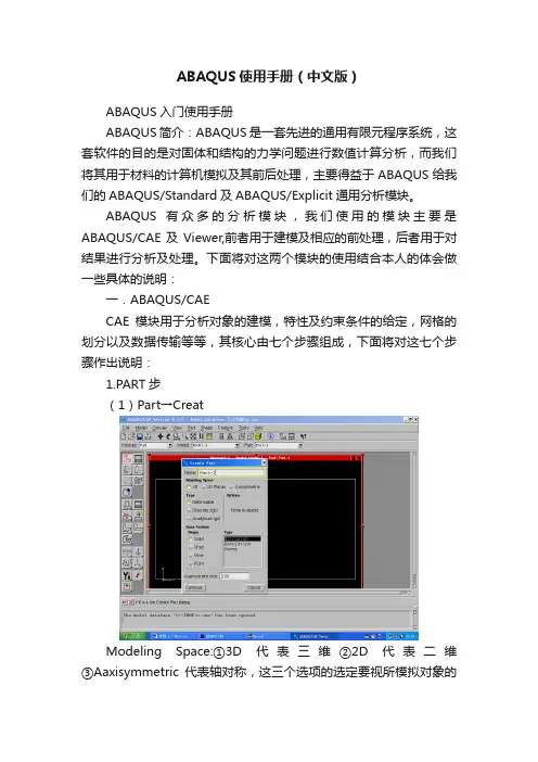
下面将对这两个模块的使用结合本人的体会做一些具体的说明：一．ABAQUS/CAECAE模块用于分析对象的建模，特性及约束条件的给定，网格的划分以及数据传输等等，其核心由七个步骤组成，下面将对这七个步骤作出说明：1.PART步（1）Part→CreatModeling Space:①3D代表三维②2D代表二维③Aaxisymmetric代表轴对称，这三个选项的选定要视所模拟对象的结构而定。

Type: ①Deformable为一般选项，适合于绝大多数的模拟对象。

②Discrete rigid 和Analytical rigid用于多个物体组合时，与我们所研究的对象相关的物体上。

ABAQUS假设这些与所研究的对象相关的物体均为刚体，对于其中较简单的刚体，如球体而言，选择前者即可。

若刚体形状较复杂，或者不是规则的几何图形，那么就选择后者。

需要说明的是，由于后者所建立的模型是离散的，所以只能是近似的，不可能和实际物体一样，因此误差较大。

Shape中有四个选项，其排列规则是按照维数而定的，可以根据我们的模拟对象确定。

Type: ①Extrusion用于建立一般情况的三维模型②Revolution建立旋转体模型③Sweep用于建立形状任意的模型。

Approximate size:在此栏中设定作图区的大致尺寸，其单位与我们选定的单位一致。

设置完毕，点击Continue进入作图区。

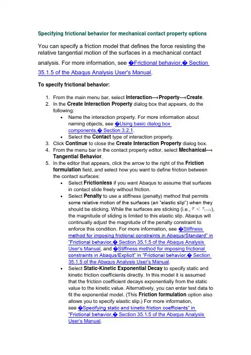
Specifying frictional behavior for mechanical contact property options You can specify a friction model that defines the force resisting the relative tangential motion of the surfaces in a mechanical contact analysis. For more information, see �Frictional behavior,�Section 35.1.5 of the Abaqus Analysis User's Manual.To specify frictional behavior:1. From the main menu bar, select Interaction Property Create.2. In the Create Interaction Property dialog box that appears, do thefollowing:∙Name the interaction property. For more information aboutnaming objects, see �Using basic dialog boxcomponents,�Section 3.2.1.∙Select the Contact type of interaction property.3. Click Continue to close the Create Interaction Property dialog box.4. From the menu bar in the contact property editor, select MechanicalTangential Behavior.5. In the editor that appears, click the arrow to the right of the Frictionformulation field, and select how you want to define friction betweenthe contact surfaces:∙Select Frictionless if you want Abaqus to assume that surfaces in contact slide freely without friction.∙Select Penalty to use a stiffness (penalty) method that permits some relative motion of the surfaces (an “elastic slip”) when theyshould be sticking. While the surfaces are sticking (i.e., ),the magnitude of sliding is limited to this elastic slip. Abaqus willcontinually adjust the magnitude of the penalty constraint toenforce this condition. For more information, see �Stiffnessmethod for imposing frictional constraints in Abaqus/Standard” in“Frictional behavior,�Section 35.1.5 of the Abaqus AnalysisUser's Manual, and �Stiffness method for imposing frictionalconstraints in Abaqus/Explicit” in “Frictional behavior,�Section35.1.5 of the Abaqus Analysis User's Manual.∙Select Static-Kinetic Exponential Decay to specify static and kinetic friction coefficients directly. In this model it is assumedthat the friction coefficient decays exponentially from the staticvalue to the kinetic value. Alternatively, you can enter test data tofit the exponential model. (This Friction formulation option alsoallows you to specify elastic slip.) For more information,see �Specifying static and kinetic friction coefficients” in“Frictional behavior,�Section 35.1.5 of the Abaqus AnalysisUser's Manual.∙Select Rough to specify an infinite coefficient of friction. For more information, see �Preventing slipping regardless ofconta ct pressure” in “Frictional behavior,�Section 35.1.5 of theAbaqus Analysis User's Manual.∙Select Lagrange Multiplier (Standard only) to enforce the sticking constraints at an interface between two surfaces usingthe Lagrange multiplier implementation. With this method there isno relative motion between two closed surfaces until .For more information, see �Lagrange multiplier method forimposing frictional constraints in Abaqus/Standard” in “Frictionalbehavior,�Section 35.1.5 of the Abaqus Analysis User'sManual.∙Select User-defined to define the shear interaction between the contact surfaces with user subroutine FRIC or VFRIC. For moreinformation, see �User-defined friction model” in “Frictionalbehavior,�Section 35.1.5 of the Abaqus Analysis User'sManual.6. If you selected the Penalty or Lagrange Multiplier (Standardonly) friction formulation, perform the following steps:a. Display the Friction tabbed page.b. Choose the Directionality:∙Choose Isotropic to enter a uniform friction coefficient.∙Choose Anisotropic (Standard only) to allow fordifferent friction coefficients in the two orthogonaldirections on the contact surface. For more information,see �Using the anisotropic friction model inAbaqus/Standard” in “Frictional behavior,�Section35.1.5 of the Abaqus Analysis User's Manual.c. Toggle on Use slip-rate-dependent data if the frictioncoefficient is dependent on slip rate.d. Toggle on Use contact-pressure-dependent data if the frictioncoefficient is dependent on the contact pressure.e. Toggle on Use temperature-dependent data if the frictioncoefficient is dependent on temperature.f. Click the arrows to the right of the Number of fieldvariables field to specify the number of field variables on whichthe friction coefficient depends.g. Enter the required data in the data table provided.h. Display the Shear Stress tabbed page, and choose a Shearstress limit option:∙Choose No limit if you do not want to limit the shearstress that can be carried by the interface before thesurfaces begin to slide.∙Choose Specify to enter an equivalent shear stresslimit, . If you choose this option, sliding will occur ifthe magnitude of the equivalent shear stress reaches thisvalue, regardless of the magnitude of the contact pressurestress. For more information, see �Using the optionalshear stress limit” in “Frictional behavior,�Section 35.1.5of the Abaqus Analysis User's Manual.i. If you selected the Penalty friction formulation, displaythe Elastic Slip tabbed page, and specify how you want todefine elastic slip:∙If you are performing an Abaqus/Standard analysis,choose an option to Specify maximum elastic slip:▪Choose Fraction of characteristic surfacedimension to calculate the allowable elastic slip asa small fraction of the characteristic contact surfacelength.▪Choose Absolute distance to enter the absolutemagnitude of the allowable elastic slip, . (For asteady-state transport analysis set this parameterequal to the absolute magnitude of the allowableelastic slip velocity () to be used in the stiffnessmethod for sticking friction.)∙If you are performing an Abaqus/Explicit analysis, choosean Elastic slip stiffness option:▪Choose Infinite (no slip) to deactivate shearsoftening.▪Choose Specify to activate softened tangentialbehavior. Enter the slope of the curve that definesthe shear traction as a function of the elastic slipbetween the two surfaces.If you selected the Static-Kinetic Exponential Decay friction formulation, perform the following steps:. Display the Friction tabbed page.a. Choose an option for defining the exponential decay frictionmodel:∙Choose Coefficients to provide the static frictioncoefficient, the kinetic friction coefficient, and the decaycoefficient directly.∙Choose Test data to provide test data points to fit theexponential model.b. If you selected the Coefficients definition option, enter thefollowing in the data table provided:∙Static friction coefficient, .∙Kinetic friction coefficient, .∙Decay coefficient, .If you selected the Test data definition option, enter the following in the data table provided:∙In the first row, enter the static friction coefficient, .∙In the second row, enter the dynamic frictioncoefficient, and the reference slip rate, , atwhich is measured.∙In the third row, enter the kinetic friction coefficient, .This value corresponds to the asymptotic value of thefriction coefficient at infinite slip rate, . If this data line isomitted, Abaqus/Standard automaticallycalculates such that .c. Display the Elastic Slip tabbed page, and specify how you wantto define elastic slip:∙If you are performing an Abaqus/Standard analysis, choose an option to Specify maximum elastic slip:▪Choose Fraction of characteristic surfacedimension to calculate the allowable elastic slip asa small fraction of the characteristic contact surfacelength.▪Choose Absolute distance to enter the absolutemagnitude of the allowable elastic slip, . (For asteady-state transport analysis set this parameterequal to the absolute magnitude of the allowableelastic slip velocity () to be used in the stiffnessmethod for sticking friction.)∙If you are performing an Abaqus/Explicit analysis, choose an Elastic slip stiffness option:▪Choose Infinite (no slip) to deactivate shearsoftening.▪Choose Specify to activate shear softening. Enterthe slope of the curve that defines the sheartraction as a function of the elastic slip between thetwo surfaces.Click OK to create the contact property and to exit the Edit Contact Property dialog box. Alternatively, you can select another contact property option to define from the menus in the Edit Contact Property dialog box.。

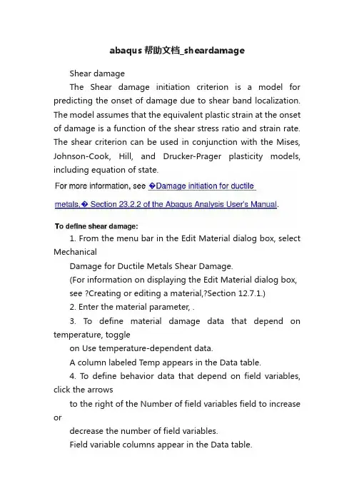
abaqus帮助文档_sheardamageShear damageThe Shear damage initiation criterion is a model for predicting the onset of damage due to shear band localization. The model assumes that the equivalent plastic strain at the onset of damage is a function of the shear stress ratio and strain rate. The shear criterion can be used in conjunction with the Mises, Johnson-Cook, Hill, and Drucker-Prager plasticity models, including equation of state.1. From the menu bar in the Edit Material dialog box, select MechanicalDamage for Ductile Metals Shear Damage.(For information on displaying the Edit Material dialog box, see ?Creating or editing a material,?Section 12.7.1.)2. Enter the material parameter, .3. To define material damage data that depend on temperature, toggleon Use temperature-dependent data.A column labeled Temp appears in the Data table.4. To define behavior data that depend on field variables, click the arrowsto the right of the Number of field variables field to increase ordecrease the number of field variables.Field variable columns appear in the Data table.5. Enter damage parameters in the Data table:Fracture StrainEquivalent fracture strain at damage initiation.Shear Stress RatioThe shear stress ratio is defined as , where q is the Mises equivalent stress, p is the pressure stress, and is the maximum shear stress.Strain RateThe equivalent plastic strain rate, .TempTemperature, .Field nPredefined field variables.You may need to expand the dialog box to see all the columns inthe Data table. For detailed information on how to enter data, see ?Entering tabular data,?Section 3.2.7.6. Select Suboptions Damage Evolution to define the materialdegradation that takes place once damage begins.For more information, see “Damage evolution.”7. Click OK to exit the material editor.。

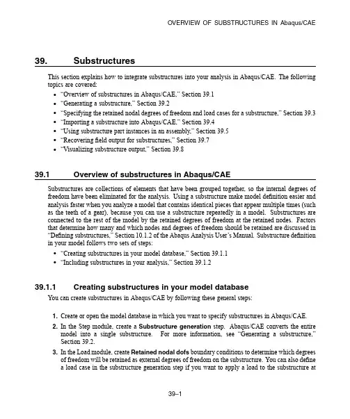
OVERVIEW OF SUBSTRUCTURES IN Abaqus/CAE39.SubstructuresThis section explains how to integrate substructures into your analysis in Abaqus/CAE.The following topics are covered:•“Overview of substructures in Abaqus/CAE,”Section39.1•“Generating a substructure,”Section39.2•“Specifying the retained nodal degrees of freedom and load cases for a substructure,”Section39.3•“Importing a substructure into Abaqus/CAE,”Section39.4•“Using substructure part instances in an assembly,”Section39.5•“Recoveringfield output for substructures,”Section39.7•“Visualizing substructure output,”Section39.839.1Overview of substructures in Abaqus/CAESubstructures are collections of elements that have been grouped together,so the internal degrees of freedom have been eliminated for the ing a substructure make model definition easier and analysis faster when you analyze a model that contains identical pieces that appear multiple times(such as the teeth of a gear),because you can use a substructure repeatedly in a model.Substructures are connected to the rest of the model by the retained degrees of freedom at the retained nodes.Factors that determine how many and which nodes and degrees of freedom should be retained are discussed in “Defining substructures,”Section10.1.2of the Abaqus Analysis User’s Manual.Substructure definition in your model follows two sets of steps:•“Creating substructures in your model database,”Section39.1.1•“Including substructures in your analysis,”Section39.1.239.1.1Creating substructures in your model databaseYou can create substructures in Abaqus/CAE by following these general steps:1.Create or open the model database in which you want to specify substructures in Abaqus/CAE.2.In the Step module,create a Substructure generation step.Abaqus/CAE converts the entiremodel into a single substructure.For more information,see“Generating a substructure,”Section39.2.3.In the Load module,create Retained nodal dofs boundary conditions to determine which degreesof freedom will be retained as external degrees of freedom on the substructure.You can also definea load case in the substructure generation step if you want to apply a load to the substructure atGENERA TING A SUBSTRUCTUREa location other than its retained degrees of freedom.For more information,see“Specifying theretained nodal degrees of freedom and load cases for a substructure,”Section39.3.4.In the Job module,create a new job and submit the analysis.When you perform an analysis of an assembly that includes substructure data,Abaqus/CAE creates separate output databases for the results of each substructure part instance and does not include the results from the substructure part instances in the output database for the assembly.The Visualization module provides tools that enable you to integrate the results from the substructure components back into the results from the assembly;for more information,see“Visualizing substructure output,”Section39.8.39.1.2Including substructures in your analysisSubstructure usage should be performed in a different model than substructure generation.You can include substructures in your analysis in Abaqus/CAE by following these general steps:1.Import each substructure that you want to use in your model database from the corresponding.simfile.For more information,see“Importing a substructure into Abaqus/CAE,”Section39.4,in the online HTML version of this manual.2.In the Assembly module,instance each substructure part that you want to add to the assembly,andposition the substructure part instances in the desired locations in the assembly.“Using substructure part instances in an assembly,”Section39.5,explains the capabilities and limitations of substructure part instances.3.In the Load module,activate substructure load cases by creating a Substructure load definition.For more information,see“Activating load cases during substructure usage,”Section39.6.4.In the Step module,create afield output request with Substructure as the Domain,then select thesubstructure sets for which you want to recoverfield data.For more information,see“Recovering field output for substructures,”Section39.7.5.In the Interaction module,apply constraints to attach the substructure part instance to the rest of theassembly.39.2Generating a substructureThefirst step in substructure definition is the addition of a Substructure generate step in your analysis.The substructure generation step enables you to create a substructure in your model database and,if desired,specify substructure-related options such as the writing of the recovery matrix,stiffness matrix, mass matrix,and load case vectors to afile.These options are described later in this section.A single analysis can include multiple substructure generate steps,and Abaqus/CAE createscorresponding output databasefiles for each step.Multiple preloading steps can precede everySPECIFYING THE RETAINED NODAL DEGREES OF FREEDOM AND LOADCASES FOR A SUBSTRUCTURE substructure generation step in your analysis.If you want to specify retained eigenmodes forsubstructure generation,you must also include a frequency extraction step in the analysis.Substructure identifierYou must specify a unique identifier for each substructure you create.Substructure identifiers must begin with the letter Z followed by a number that cannot exceed999.Recovery optionsYou can recover thefield output data for a substructure during the usage-level analysis,but you must specify the recovery region during substructure generation.Substructure recovery can be performed only on the sets included in the recovery region.You can specify that recovery be performed on the whole model or for an individual node set or element set.While performing the substructure recovery in the usage model,Abaqus/CAE must have access to the substructure’s.mdl,.prt, .stt,and.supfiles.For more information about thesefile types,see“Defining substructures,”Section10.1.2of the Abaqus Analysis User’s Manual.Generation optionsYou can control several aspects of the substructure generation process,including calculation of gravity load vectors,evaluation of frequency-dependent material properties,and generation of a reduced mass matrix,reduced structural damping matrix,and viscous damping matrix.Retained eigenmodesYou can specify retained eigenmodes for generation of a coupled acoustic-structural substructure.When you choose to specify retained eigenmodes,Abaqus/CAE enables you to specify eigenmodes by mode range or by frequency range.DampingYou can specify several global damping controls and substructure damping controls.For global damping you can choose to apply damping settings to acoustic or mechanical options;for substructure damping you can specify separate controls for viscous and structural damping. 39.3Specifying the retained nodal degrees of freedom and load casesfor a substructureAfter you defined the substructure generation step or steps for your analysis,you must define a Retained nodal dofs boundary condition for a substructure.The retained degrees of freedom for a substructure node are the degrees of freedom that are external and are available for use in the analysis;all other degrees of freedom for the specified node are assumed to be internal to the substructure and do not factor into the analysis.When you import a substructure from this analysis into a model for substructure usage, Abaqus/CAE displays these nodes as light blue crosses,which enables you to pick them easily from a part instance or assembly.ACTIVA TING LOAD CASES DURING SUBSTRUCTURE USAGEIf you want to apply a load to the substructure at a location other than its retained degrees of freedom, you can define a load case in the substructure generation step.39.4Importing a substructure into Abaqus/CAEYou can include substructure definitions in a model database and begin to use them for modeling by importing the substructures as new part definitions.Substructure data are available in.simfiles, and the substructure identifier is included in thefile name;for example,in an analysis in which the substructure is named FAN and the substructure identifier is Z400,the substructure databasefile is named FAN_Z400.sim.The.simfile from which you import a substructure must reside in the same directory as the supporting Abaqusfiles to which the.sim database refers;these supportingfiles may include data in the formats.prt,.mdl,.stt,or.sup.Substructure import also requires an output database(.odb)file for mesh display.39.5Using substructure part instances in an assemblyOnce you import substructure parts into your model database,you can add them to your assembly by instancing them in the same manner you would for any part.Substructure part instances are displayed in a translucent color in the viewport.You can move and apply constraints to substructure part instances;however,substructure part instances have the following modeling limitations:•You cannot assign sections to a substructure part instance.•You cannot apply attributes to a substructure part instance.•Substructure part instances are not eligible for definition of contact pairs.•Gravity loads are the only load definition that can be applied to substructure part instances. 39.6Activating load cases during substructure usageThe Substructure load definition enables you to activate the substructure load cases that are specified during the substructure generation step.As you activate a load case,you can scale its load definitions or apply an amplitude to them.VISUALIZING SUBSTRUCTURE OUTPUT39.7Recovering field output for substructuresYou can specify that Abaqus/CAE writefield output data for one or more substructure sets in your analysis.From thefield output editor,select Substructure from the Domainfield,then click to open the Select Substructure Sets dialog box.This dialog box lists only the substructure sets that were defined while generating the substructure.You cannot recover data for sets that you define on substructure part instances in Abaqus/CAE.39.8Visualizing substructure outputAbaqus/CAE creates separate output database(.odb)files for each substructure part instance used in the analysis,so you must perform some additional steps if you want to display substructure results in context with the rest of the assembly.The Visualization module provides the following tools that enable you to incorporate substructure results into the rest of the model:•You can use an overlay plot to display plots of substructure data in the same viewport as a plot of the rest of the assembly.•You can use the Combine ODBs plug-in to combine the data in one or more substructure output databasefiles with the data from the rest of the assembly.。

abaqus帮助文档水力压裂例子inp文件解释10.1.5-副本（53）预览说明:预览图片所展示的格式为文档的源格式展示,下载源文件没有水印,内容可编辑和复制**约束底面单元u3=0*Amplitude, name=volumerate振幅，名称=volumerate0.0,0.0, 200.0,-1.0**时间或频率，幅值1；时间或频率，幅值2**STEP ----------------------------------------------------------------**** STEP: Step-1***Step, name=Step-1, nlgeom=YES, unsymm=YESNlgeom选择ON表示计算中加入几何非线性。

材料力学和弹性力学的一项基本假设是材料的位移与应变关系是线性的,且应变为小量,即几何关系是线性的,属于小变形问题。

UNSYMM:设置UNSYMM=YES表明使用非对称矩阵存储求解。

设置=NO表明使用对称矩阵存储求解。

该参数的默认值依赖于模型和求解序列*Geostatic**初始应力平衡**** LOADS加载**** Name: Load-1 Type: Pressure名称：Load-1 类型：Pressure*Dsload_PickedSurf260, P, 42000.**顶面施加42000的垂向压力：表面名，分布载荷类型标签，参考载荷大小** Name: Load-2 Type: Body force名称：Load-2 类型：Body force（体力）*Dload_PickedSet8, BZ, -20.**所有单元施加向下的分布力20** Name: Load-3 Type: Pressure*Dsloadwell_bore, PNU, 1.**井筒上的分布载荷，user-defined？井眼，PNU,1***Boundary,user**边界，在子程序disp中定义**_PickedSet5, 8, 8, 1TOP, 8, 8, 1**顶面所有点，8,8——孔隙压力（或静水压），变量大小BOT, 8, 8, 1**底面所有点**。

Abaqus使用日记Abaqus标准版共有“部件（part）”、“材料特性（propoterty）”、“装配（assemble）”、“计算步骤（step）”、“交互（interaction）”、“加载（load）”、“单元划分（mesh）”、“计算（job）”、“后处理（visualization）”、“草图（sketch）”十大模块组成。

建模方法：一个模型（model）通常由一个或几个部件（part）组成，“部件”又由一个或几个特征体（feature）组成，每一个部分至少有一个基本特征体（base feature），特征体可以是所创建的实体，如挤压体、切割挤压体、数据点、参考点、数据轴，数据平面，装配体的装配约束、装配体的实例等等。

1．首先建立“部件”（1）根据实际模型的尺寸决定部件的近似尺寸，进入绘图区。

绘图区根据所输入的近似尺寸决定网格的间距，间距大小可以在edit菜单sketcher options选项里调整。

（2）在绘图区分别建立部件中的各个特征体，建立特征体的方法主要有挤压、旋转、平扫三种。

同一个模型中两个不同的部件可以有同名的特征体组成，也就是说不同部件中可以有同名的特征体，同名特征体可以相同也可以不同。

部件的特征体包括用各种方法建立的基本特征体、数据点（datum point）、数据轴（datum axis）、数据平面（datum plane）等等。

（3）编辑部件可以用部件管理器进行部件复制，重命名，删除等，部件中的特征体可以是直接建立的特征体，还可以间接手段建立，如首先建立一个数据点特征体，通过数据点建立数据轴特征体，然后建立数据平面特征体，再由此基础上建立某一特征体，最先建立的数据点特征体就是父特征体，依次往下分别为子特征体，删除或隐藏父特征体其下级所有子特征体都将被删除或隐藏。

××××特征体被删除后将不能够恢复，一个部件如果只包含一个特征体，删除特征体时部件也同时被删除×××××2．建立材料特性（1）输入材料特性参数弹性模量、泊松比等（2）建立截面（section）特性，如均质的、各项同性、平面应力平面应变等等，截面特性管理器依赖于材料参数管理器（3）分配截面特性给各特征体，把截面特性分配给部件的某一区域就表示该区域已经和该截面特性相关联3．建立刚体（1）部件包括可变形体、不连续介质刚体和分析刚体三种类型，在创建部件时需要指定部件的类型，一旦建立后就不能更改其类型。

Abaqus基本操作中文教程目录1 Abaqus软件基本操作 (3)1.1 常用的快捷键 (3)1.2 单位的一致性 (3)1.3 分析流程九步走 (3)1.3.1 几何建模（Part） (4)1.3.2 属性设置（Property） (5)1.3.3 建立装配体（Assembly） (6)1.3.4 定义分析步（Step） (7)1.3.5 相互作用（Interaction） (8)1.3.6 载荷边界（Load） (10)1.3.7 划分网格（Mesh） (11)1.3.8 作业（Job） (15)1.3.9 可视化（Visualization） (16)1 Abaqus软件基本操作1.1 常用的快捷键旋转模型—Ctrl+Alt+鼠标左键平移模型—Ctrl+Alt+鼠标中键1.2 单位的一致性CAE软件其实是数值计算软件，没有单位的概念，常用的国际单位制如下表1所示，建议采用SI (mm)进行建模。

例如，模型的材料为钢材，采用国际单位制SI (m)时，弹性模量为2.06e11N/m2，重力加速度9.800 m/s2，密度为7850 kg/m3，应力Pa；采用国际单位制SI (mm)时，弹性模量为2.06e5N/mm2，重力加速度9800 mm/s2，密度为7850e-12 T/mm3，应力MPa。

1.3 分析流程九步走几何建模（Part）→属性设置（Property）→建立装配体（Assembly）→定义分析步（Step）→相互作用（Interaction）→载荷边界（Load）→划分网格（Mesh）→作业（Job）→可视化（Visualization）1.3.1 几何建模（Part ） 关键步骤的介绍： 部件（Part ）导入Pro/E 等CAD 软件建好的模型后，另存成iges 、sat 、step 等格式；然后导入Abaqus 可以直接用，实体模型的导入通常采用sat 格式文件导入。

部件（Part ）创建简单的部件建议直接在abaqus 中完成创建，复杂的可以借助Pro/E 或者Solidworks 等专业软件进行建模，然后导入。

(一)总规则1、关键词必须以*符号开头，且关键词前无空格；2、**为解释行，它可以出现在文件中的任何地方；2、当关键词后带有参数时，关键词后必须采用逗号相隔；3、参数间采用都好相隔；4、关键词可以采用简写的方式，只要程序能够识别就可以了；5、没有隔行符，如果参数比较多，一行放不下，可以另起一行，只要在上一行的末尾加逗号便可以；(二)建模部分关键词在我的学习过程中，是将ansys的模型倒入abaqus的，最简单的方法就是在ansys中提取单元与节点信息，将提取出来的信息在abaqus中形成有限元模型。

因此首先从节点的关键词来开始吧。

1、*heading描述行这是.inp文件的开头语，相当于你告诉abaqus，我要进行工程建模与分析了。

另起一行可以对模型进行描述，这个描述可有可无，只是为了以后阅读的方便。

abaqus中对每个模块没有清晰的界定，根据关键词的不同来判别进入哪个模块。

而在ansys中对模块要求比较严格，如/prep7为前处理模块，/solu为求解模块,/post26为后处理模块。

2、*node,<input>,<nset=结点集名称>,<system>数据行(a) 通知软件，我要开始建立结点了。

<>的意思是<>中的内容可有可无，这两个也称为node 命令的参数。

(b) <input>: 指出包含结点所在的文件名称，包括文件的扩展名。

当这项参数省略时，程序认为*node下的数据为所需要建立的结点。

(c) <nset=结点集名称>: 熟悉ansys的人应该了解，为了选择的方便对某些合适的点可以采用cm命令建立component(cm,结点集名称,node)，在abaqus中<nset=结点集名称>与此相对应。

abaqus中英文ABAQUS专业术语中英文对照前后处理器模块——ABAQUS/CAE几何体建模——GeometryGeometry Creation Tools（几何体生成工具）2-D Sketcher（二维草图）Sketch T ools and Options（草图工具和选项）Geometry Import/Export（几何体导入和导出）Geometry Repair T ools（几何体修补工具）Mesh Edit（网格编辑）模型装配——AssemblyInstance Tools（实例工具）Sets and Surfaces（集合和表面）Display Groups（显式组）Merge/Cut T ools（合并/剪切操作）定义材料性质——PropertiesMaterial Models（材料模型）General（一般性质）Elasticity（弹性性质）Electrical properties(电性质)Mass diffusion（质量扩散）Plasticity（塑性性质）Pore fluid properties（孔隙流体性质）Thermal properties（热性质）Gasket（垫片）Acoustic medium（声学介质）Equation of state (EOS) materials（状态方程）User materials（用户自定义材料）Hyperelastic material evaluation（超弹性材料评估）Sections（截面性质）Solid（实体）homogeneous（各向同性的）, generalized plane strain（广义平面应变的Shell（壳）homogeneous（各向同性的）, composite（复合材料壳单元）, membrane （薄膜）,surface (rebar layers)（带钢筋层的曲面）Beam（梁） beam（梁）, truss（杆）Point（点）mass（质量单元）, rotary inertia（转动惯量）, damping（阻尼）, capacitance（电容）Gasket（垫片）Beam section profiles（梁截面形状）Skin（蒙皮）Orientations（材料方向）分析流程功能——AnalysisGeneral, Linear and Nonlinear Analyses（通用，线性和非线性分析）Static stress/displacement analysis（静力分析）Viscoelastic/viscoplastic response（粘弹/粘塑响应）Dynamic stress/displacement analysis（动力分析）Heat transfer analysis（热传导分析）Mass diffusion analysis（质量扩散分析）Acoustic analysis（声学分析）Coupled problems（耦合问题）– Thermo-mechanical（热固）– Thermo-electrical（热电）– Piezoelectric（压电）– Pore fluid flow-mechanical（孔隙流动）– Thermo-mechanical mass diffusion（热-固-质量扩散）– Shock and acoustic-structural（冲击和声固耦合）Linear Perturbation Analyses（线性摄动分析）Static stress/displacement analysis（应力位移静力分析）– Linear static stress/displacement analysis（应力位移线性静力分析）– Eigenvalue buckling estimates（特征值屈曲分析）Dynamic stress/displacement analysis（应力位移动力学分析）– Natural frequency extraction（自振频率提取）– Complex eigenvalue extraction（复频率提取）– Transient response via modal superposition（通过模态叠加法计算瞬态响应）–Steady-state response to harmonic loading （简谐载荷下的稳态响应）– Response spectrum analysis（响应谱分析）– Random response analysis（随机响应分析）Analysis Controls（分析控制）Output Requests（输出请求）定义约束和接触——Constraints and InteractionsContact（接触）General contact (ABAQUS/Explicit)（通用接触）Surface-to-surface contact（面面接触）Self-contact（自接触）Contact Properties（接触性质）Constraints（约束）Thermal（热）Loads（载荷）Mechanical（机械）Bolt load（螺栓预紧力）Thermal（热）Acoustic（声场）Fluid（流体）Electrical（电）Mass diffusion（质量扩散）Fields（场）Multiple load cases（多工况）Connectors（连接单元）Boundary Conditions（边界条件）Nodal（节点位移）Velocity（速度）Acceleration（加速度）Velocity/angular velocity（角速度）Submodel（子模型）Pore pressure（孔压）Electric potential（电势）Temperatures（温度）网格划分——MeshingMesh Seeding（网格种子）Structured Meshing（结构化分网）Surface Meshing（表面分网）Solid Meshing（实体分网）Virtual Topology（虚拟拓扑）单元库——Element Library Beam（梁单元）Truss（杆单元）Connector（连接单元）Shell（壳单元）Membrane（薄膜单元）Continuum（实体单元）Elbow（弯管单元）Gasket（垫片单元）Pipe（管道单元）后处理——VisualizationModel plotting（模型图）Deformed, contour, vector/tensor, path, tickmark, overlay, material orient ations, X–Y plots（变形图，云图、矢量/张量图、材料方向图、X-Y曲线图等）Animations（动画）Stress linearization（应力线性化）Tabular data reports（数据报表）Probe/query tools（查询工具）Diagnostics visualization（结果诊断）过程自动化——Process AutomationPython scripting（Python脚本）GUI toolkit（用户界面工具包）Macro manager（宏管理器）隐式求解器模块——ABAQUS/STANDARD分析类型——Analysis TypesGeneral, Linear and Nonlinear Analyses（通用，线性和非线性分析） Static stress/displacement analysis（静力分析）Direct cyclic analysis（直接载荷循环分析）Viscoelastic/viscoplastic response（粘弹性和粘塑性）Dynamic stress/displacement analysis（动力学分析）Steady-state transport analysis（稳态传输分析）Heat transfer analysis（热传导分析）Mass diffusion analysis（质量扩散分析）Acoustic analysis（声场分析）Coupled analysis（耦合分析）Linear Perturbation Analyses（线性摄动分析）分析和建模技术——Analysis and Modeling Techniques求解技术——Solution Techniques材料定义——Material DefinitionsElastic Mechanical Properties（弹性机械性质）Inelastic Mechanical Properties（非弹性机械性质）Additional Material Properties（其他材料性质）单元库——Element LibraryContinuum（实体单元）Membranes（薄膜单元）Beams（梁单元）Pipes（管道单元）Elbows（弯管单元）Frame Elements（框架单元）Trusses（杆单元）Gasket Elements（垫片单元）Inertial Elements（惯性单元）Rigid Elements（刚体单元）Capacitance Elements（热容单元）Connector Elements（连接单元）Springs, Dashpots, Flexible Joints（弹簧，阻尼器，柔性接头）Distributed Coupling（分布耦合）Special-Purpose Elements（特殊用途单元）User-Defined Elements（用户自定义单元）预设条件——Prescribed Conditions约束和接触——Constraints and Interactions Kinematic Constraints（自由度约束）Surface-Based Contact Modeling（基于表面的接触建模）Element-Based Contact Modeling（基于单元的接触建模）Cavity Radiation（空腔辐射）用户子程序——User Subroutines显式求解器模块——ABAQUS/EXPLICIT分析类型——Analysis Types非线性显示动力学分析分析和建模技术——Analysis and Modeling Techniques 材料定义——Material DefinitionsElastic Mechanical Properties（弹性机械性质）Inelastic Mechanical Properties（非弹性机械性质）Additional Material Properties（其他材料性质）单元库——Element LibraryContinuum（实体单元）Structural（结构单元）Inertial Elements（惯性单元）Rigid Elements（刚体单元）Capacitance Elements（热容单元）Connector Elements（连接单元）Springs, Dashpots（弹簧和阻尼器）预设条件——Prescribed Conditions约束和接触——Constraints and InteractionsKinematic Constraints（自由度约束）Contact Modeling（接触建模）。

ABAQUS使用手册（中文版）abaqus入门使用手册abaqus简介：abaqus是一套先进的通用有限元程序系统，这套软件的目的是对固体和结构的力学问题进行数值计算分析，而我们将其用于材料的计算机模拟及其前后处理，主要得益于abaqus给我们的abaqus/standard及abaqus/explicit通用分析模块。

abaqus存有众多的分析模块，我们采用的模块主要就是abaqus/cae及viewer,前者用作建模及适当的前处置，后者用作对结果展开分析及处置。

下面将对这两个模块的采用融合本人的体会搞一些具体内容的表明：一．abaqus/caecae模块用于分析对象的建模，特性及约束条件的给定，网格的划分以及数据传输等等，其核心由七个步骤组成，下面将对这七个步骤作出说明：1.part步（1）part→creatmodelingspace:①3d代表三维②2d代表二维③aa xisymmetric代表轴对称，这三个选项的选取视乎所演示对象的结构而的定。

type:①deformable为一般选项，适合于绝大多数的模拟对象。

②discreterigid和analyticalrigid用于多个物体组合时，与我们所研究的对象相关的物体上。

abaqus假设这些与所研究的对象相关的物体均为刚体，对于其中较简单的刚体，如球体而言，选择前者即可。

若刚体形状较复杂，或者不是规则的几何图形，那么就选择后者。

需要说明的是，由于后者所建立的模型是离散的，所以只能是近似的，不可能和实际物体一样，因此误差较大。

shape中存有四个选项，其排序规则就是按照维数而的定的，可以根据我们的演示对象确认。

1type:①extrusion用作创建通常情况的三维模型②revolution创建旋转体模型③sweep用作创建形状任一的模型。

approximatesize:在此栏中设定作图区的大致尺寸，其单位与我们选定的单位一致。

设置完，页面continue步入作图区。

Abaqus 使用日记Abaqus标准版共有“部件（part）”、“材料特性（propoterty）”、“装配（assemble）”、“计算步骤（step）”、“交互（interaction）”、“加载（load）”、“单元划分（mesh）”、“计算（job）”、“后处理（visualization）”、“草图（sketch）”十大模块组成。

建模方法：一个模型（model）通常由一个或几个部件（part）组成，“部件”又由一个或几个特征体（feature）组成，每一个部分至少有一个基本特征体（base feature），特征体可以是所创建的实体，如挤压体、切割挤压体、数据点、参考点、数据轴，数据平面，装配体的装配约束、装配体的实例等等。

1．首先建立“部件”（1）根据实际模型的尺寸决定部件的近似尺寸，进入绘图区。

绘图区根据所输入的近似尺寸决定网格的间距，间距大小可以在edit菜单sketcher options选项里调整。

（2）在绘图区分别建立部件中的各个特征体，建立特征体的方法主要有挤压、旋转、平扫三种。

同一个模型中两个不同的部件可以有同名的特征体组成，也就是说不同部件中可以有同名的特征体，同名特征体可以相同也可以不同。

部件的特征体包括用各种方法建立的基本特征体、数据点（datum point）、数据轴（datum axis）、数据平面（datum plane）等等。

（3）编辑部件可以用部件管理器进行部件复制，重命名，删除等，部件中的特征体可以是直接建立的特征体，还可以间接手段建立，如首先建立一个数据点特征体，通过数据点建立数据轴特征体，然后建立数据平面特征体，再由此基础上建立某一特征体，最先建立的数据点特征体就是父特征体，依次往下分别为子特征体，删除或隐藏父特征体其下级所有子特征体都将被删除或隐藏。

××××特征体被删除后将不能够恢复，一个部件如果只包含一个特征体，删除特征体时部件也同时被删除×××××2．建立材料特性（1）输入材料特性参数弹性模量、泊松比等（2）建立截面（section）特性，如均质的、各项同性、平面应力平面应变等等，截面特性管理器依赖于材料参数管理器（3）分配截面特性给各特征体，把截面特性分配给部件的某一区域就表示该区域已经和该截面特性相关联3．建立刚体（1）部件包括可变形体、不连续介质刚体和分析刚体三种类型，在创建部件时需要指定部件的类型，一旦建立后就不能更改其类型。

Specifying frictional behavior for mechanical contact property options You can specify a friction model that defines the force resisting the relative tangential motion of the surfaces in a mechanical contact analysis. For more information, see �Frictional behavior,�Section 35.1.5 of the Abaqus Analysis User's Manual.To specify frictional behavior:1. From the main menu bar, select Interaction Property Create.2. In the Create Interaction Property dialog box that appears, do thefollowing:∙Name the interaction property. For more information aboutnaming objects, see �Using basic dialog boxcomponents,�Section 3.2.1.∙Select the Contact type of interaction property.3. Click Continue to close the Create Interaction Property dialog box.4. From the menu bar in the contact property editor, select MechanicalTangential Behavior.5. In the editor that appears, click the arrow to the right of the Frictionformulation field, and select how you want to define friction betweenthe contact surfaces:∙Select Frictionless if you want Abaqus to assume that surfaces in contact slide freely without friction.∙Select Penalty to use a stiffness (penalty) method that permits some relative motion of the surfaces (an “elastic slip”) when theyshould be sticking. While the surfaces are sticking (i.e., ),the magnitude of sliding is limited to this elastic slip. Abaqus willcontinually adjust the magnitude of the penalty constraint toenforce this condition. For more information, see �Stiffnessmethod for imposing frictional constraints in Abaqus/Standard” in“Frictional behavior,�Section 35.1.5 of the Abaqus AnalysisUser's Manual, and �Stiffness method for imposing frictionalconstraints in Abaqus/Explicit” in “Frictional behavior,�Section35.1.5 of the Abaqus Analysis User's Manual.∙Select Static-Kinetic Exponential Decay to specify static and kinetic friction coefficients directly. In this model it is assumedthat the friction coefficient decays exponentially from the staticvalue to the kinetic value. Alternatively, you can enter test data tofit the exponential model. (This Friction formulation option alsoallows you to specify elastic slip.) For more information,see �Specifying static and kinetic friction coefficients” in“Frictional behavior,�Section 35.1.5 of the Abaqus AnalysisUser's Manual.∙Select Rough to specify an infinite coefficient of friction. For more information, see �Preventing slipping regardless ofconta ct pressure” in “Frictional behavior,�Section 35.1.5 of theAbaqus Analysis User's Manual.∙Select Lagrange Multiplier (Standard only) to enforce the sticking constraints at an interface between two surfaces usingthe Lagrange multiplier implementation. With this method there isno relative motion between two closed surfaces until .For more information, see �Lagrange multiplier method forimposing frictional constraints in Abaqus/Standard” in “Frictionalbehavior,�Section 35.1.5 of the Abaqus Analysis User'sManual.∙Select User-defined to define the shear interaction between the contact surfaces with user subroutine FRIC or VFRIC. For moreinformation, see �User-defined friction model” in “Frictionalbehavior,�Section 35.1.5 of the Abaqus Analysis User'sManual.6. If you selected the Penalty or Lagrange Multiplier (Standardonly) friction formulation, perform the following steps:a. Display the Friction tabbed page.b. Choose the Directionality:∙Choose Isotropic to enter a uniform friction coefficient.∙Choose Anisotropic (Standard only) to allow fordifferent friction coefficients in the two orthogonaldirections on the contact surface. For more information,see �Using the anisotropic friction model inAbaqus/Standard” in “Frictional behavior,�Section35.1.5 of the Abaqus Analysis User's Manual.c. Toggle on Use slip-rate-dependent data if the frictioncoefficient is dependent on slip rate.d. Toggle on Use contact-pressure-dependent data if the frictioncoefficient is dependent on the contact pressure.e. Toggle on Use temperature-dependent data if the frictioncoefficient is dependent on temperature.f. Click the arrows to the right of the Number of fieldvariables field to specify the number of field variables on whichthe friction coefficient depends.g. Enter the required data in the data table provided.h. Display the Shear Stress tabbed page, and choose a Shearstress limit option:∙Choose No limit if you do not want to limit the shearstress that can be carried by the interface before thesurfaces begin to slide.∙Choose Specify to enter an equivalent shear stresslimit, . If you choose this option, sliding will occur ifthe magnitude of the equivalent shear stress reaches thisvalue, regardless of the magnitude of the contact pressurestress. For more information, see �Using the optionalshear stress limit” in “Frictional behavior,�Section 35.1.5of the Abaqus Analysis User's Manual.i. If you selected the Penalty friction formulation, displaythe Elastic Slip tabbed page, and specify how you want todefine elastic slip:∙If you are performing an Abaqus/Standard analysis,choose an option to Specify maximum elastic slip:▪Choose Fraction of characteristic surfacedimension to calculate the allowable elastic slip asa small fraction of the characteristic contact surfacelength.▪Choose Absolute distance to enter the absolutemagnitude of the allowable elastic slip, . (For asteady-state transport analysis set this parameterequal to the absolute magnitude of the allowableelastic slip velocity () to be used in the stiffnessmethod for sticking friction.)∙If you are performing an Abaqus/Explicit analysis, choosean Elastic slip stiffness option:▪Choose Infinite (no slip) to deactivate shearsoftening.▪Choose Specify to activate softened tangentialbehavior. Enter the slope of the curve that definesthe shear traction as a function of the elastic slipbetween the two surfaces.If you selected the Static-Kinetic Exponential Decay friction formulation, perform the following steps:. Display the Friction tabbed page.a. Choose an option for defining the exponential decay frictionmodel:∙Choose Coefficients to provide the static frictioncoefficient, the kinetic friction coefficient, and the decaycoefficient directly.∙Choose Test data to provide test data points to fit theexponential model.b. If you selected the Coefficients definition option, enter thefollowing in the data table provided:∙Static friction coefficient, .∙Kinetic friction coefficient, .∙Decay coefficient, .If you selected the Test data definition option, enter the following in the data table provided:∙In the first row, enter the static friction coefficient, .∙In the second row, enter the dynamic frictioncoefficient, and the reference slip rate, , atwhich is measured.∙In the third row, enter the kinetic friction coefficient, .This value corresponds to the asymptotic value of thefriction coefficient at infinite slip rate, . If this data line isomitted, Abaqus/Standard automaticallycalculates such that .c. Display the Elastic Slip tabbed page, and specify how you wantto define elastic slip:∙If you are performing an Abaqus/Standard analysis, choose an option to Specify maximum elastic slip:▪Choose Fraction of characteristic surfacedimension to calculate the allowable elastic slip asa small fraction of the characteristic contact surfacelength.▪Choose Absolute distance to enter the absolutemagnitude of the allowable elastic slip, . (For asteady-state transport analysis set this parameterequal to the absolute magnitude of the allowableelastic slip velocity () to be used in the stiffnessmethod for sticking friction.)∙If you are performing an Abaqus/Explicit analysis, choose an Elastic slip stiffness option:▪Choose Infinite (no slip) to deactivate shearsoftening.▪Choose Specify to activate shear softening. Enterthe slope of the curve that defines the sheartraction as a function of the elastic slip between thetwo surfaces.Click OK to create the contact property and to exit the Edit Contact Property dialog box. Alternatively, you can select another contact property option to define from the menus in the Edit Contact Property dialog box.。

1.1.41 UMATUser subroutine to define a material's mechanical behavior.Product: Abaqus/StandardWarning: The use of this subroutine generally requires considerable expertise. Y ou arecautioned that the implementation of any realistic constitutive model requires extensivedevelopment and testing. Initial testing on a single-element model with prescribedtraction loading is strongly recommended.References“User-defined mechanical material behavior,” Section 26.7.1 of the Abaqus Analysis User's Guide“User-defined thermal material behavior,” Section 26.7.2 of the Abaqus Analysis User's Guide*USER MA TERIAL“S D V I N I,” Section 4.1.11 of the Abaqus V erification Guide“U M A T and U H Y P E R,” Section 4.1.21 of the Abaqus V erification GuideOv erv iewUser subroutine U M A T:can be used to define the mechanical constitutive behavior of a material;will be called at all material calculation points of elements for which the material definition includes auser-defined material behavior;can be used with any procedure that includes mechanical behavior;can use solution-dependent state variables;must update the stresses and solution-dependent state variables to their values at the end of theincrement for which it is called;must provide the material Jacobian matrix, , for the mechanical constitutive model;can be used in conjunction with user subroutine U S D F L D to redefine any field variables before they are passed in; andis described further in “User-defined mechanical material behavior,” Section 26.7.1 of the AbaqusAnalysis User's Guide.Storage of stress and strain componentsIn the stress and strain arrays and in the matrices D D S D D E, D D S D D T, and D R P L D E, direct components are stored first, followed by shear components. There are N D I direct and N S H R engineering shear components. The order of the components is defined in “Conventions,” Section 1.2.2 of the Abaqus Analysis User's Guide. Since the number of active stress and strain components varies between element types, the routine must be coded toprovide for all element types with which it will be used.Defining local orientationsIf a local orientation (“Orientations,” Section 2.2.5 of the Abaqus Analysis User's Guide) is used at the same point as user subroutine U M A T, the stress and strain components will be in the local orientation; and, in the case of finite-strain analysis, the basis system in which stress and strain components are stored rotates with the material.StabilityY ou should ensure that the integration scheme coded in this routine is stable—no direct provision is made to include a stability limit in the time stepping scheme based on the calculations in U M A T.Convergence rateD D S D DE and—for coupled temperature-displacement and coupled thermal-electrical-structural analyses—D D S D D T, D R P L D E, and D R P L D T must be defined accurately if rapid convergence of the overall Newton scheme is to be achieved. In most cases the accuracy of this definition is the most important factor governing the convergence rate. Since nonsymmetric equation solution is as much as four times as expensive as the corresponding symmetric system, if the constitutive Jacobian (D D S D D E) is only slightly nonsymmetric (for example, a frictional material with a small friction angle), it may be less expensive computationally to use a symmetric approximation and accept a slower convergence rate.An incorrect definition of the material Jacobian affects only the convergence rate; the results (if obtained) are unaffected.Special considerations for various element typesThere are several special considerations that need to be noted.A v ailability of deformation gradientThe deformation gradient is available for solid (continuum) elements, membranes, and finite-strain shells(S3/S3R, S4, S4R, SAXs, and SAXAs). It is not available for beams or small-strain shells. It is stored as a 3× 3 matrix with component equivalence D F G R D0(I,J). For fully integrated first-order isoparametric elements (4-node quadrilaterals in two dimensions and 8-node hexahedra in three dimensions) the selectively reduced integration technique is used (also known as the technique). Thus, a modified deformation gradientis passed into user subroutine U M A T. For more details, see “Solid isoparametric quadrilaterals and hexahedra,”Section 3.2.4 of the Abaqus Theory Guide.Beams and shells that calculate transv erse shear energyIf user subroutine U M A T is used to describe the material of beams or shells that calculate transverse shear energy, you must specify the transverse shear stiffness as part of the beam or shell section definition to define the transverse shear behavior. See “Shell section behavior,” Section 29.6.4 of the Abaqus Analysis User's Guide, and “Choosing a beam element,” Section 29.3.3 of the Abaqus Analysis User's Guide, for informationon specifying this stiffness.Open-section beam elementsWhen user subroutine U M A T is used to describe the material response of beams with open sections (for example, an I-section), the torsional stiffness is obtained aswhere J is the torsional constant, A is the section area, k is a shear factor, and is the user-specified transverse shear stiffness (see “Transverse shear stiffness definition” in “Choosing a beam element,” Section29.3.3 of the Abaqus Analysis User's Guide).E lements w ith hourglassing modesIf this capability is used to describe the material of elements with hourglassing modes, you must define the hourglass stiffness factor for hourglass control based on the total stiffness approach as part of the element section definition. The hourglass stiffness factor is not required for enhanced hourglass control, but you can define a scaling factor for the stiffness associated with the drill degree of freedom (rotation about the surface normal). See “Section controls,” Section 27.1.4 of the Abaqus Analysis User's Guide, for information on specifying the stiffness factor.Pipe-soil interaction elementsThe constitutive behavior of the pipe-soil interaction elements (see “Pipe-soil interaction elements,” Section 32.12.1 of the Abaqus Analysis User's Guide) is defined by the force per unit length caused by relative displacement between two edges of the element. The relative-displacements are available as “strains” (S T R A N and D S T R A N). The corresponding forces per unit length must be defined in the S T R E S S array. The Jacobian matrix defines the variation of force per unit length with respect to relative displacement.For two-dimensional elements two in-plane components of “stress” and “strain” exist (N T E N S=N D I=2, andN S H R=0). For three-dimensional elements three components of “stress” and “strain” exist (N T E N S=N D I=3, and N S H R=0).Large volume changes with geometric nonlinearityIf the material model allows large volume changes and geometric nonlinearity is considered, the exact definition of the consistent Jacobian should be used to ensure rapid convergence. These conditions are most commonly encountered when considering either large elastic strains or pressure-dependent plasticity. In the former case, total-form constitutive equations relating the Cauchy stress to the deformation gradient are commonly used; in the latter case, rate-form constitutive laws are generally used.For total-form constitutive laws, the exact consistent Jacobian is defined through the variation in Kirchhoff stress:Here, J is the determinant of the deformation gradient, is the Cauchy stress, is the virtual rate of deformation, and is the virtual spin tensor, defined asFor rate-form constitutive laws, the exact consistent Jacobian is given byUse with incompressible elastic materialsFor user-defined incompressible elastic materials, user subroutine U H Y P E R should be used rather than user subroutine U M A T. In U M A T incompressible materials must be modeled via a penalty method; that is, you must ensure that a finite bulk modulus is used. The bulk modulus should be large enough to model incompressibility sufficiently but small enough to avoid loss of precision. As a general guideline, the bulk modulus should be about – times the shear modulus. The tangent bulk modulus can be calculated fromIf a hybrid element is used with user subroutine U M A T, Abaqus/Standard will replace the pressure stress calculated from your definition of S T R E S S with that derived from the Lagrange multiplier and will modify the Jacobian appropriately.For incompressible pressure-sensitive materials the element choice is particularly important when using user subroutine U M A T. In particular, first-order wedge elements should be avoided. For these elements the technique is not used to alter the deformation gradient that is passed into user subroutine U M A T, which increases the risk of volumetric locking.Increments for which only the Jacobian can be definedAbaqus/Standard passes zero strain increments into user subroutine U M A T to start the first increment of all the steps and all increments of steps for which you have suppressed extrapolation (see “Defining an analysis,”Section 6.1.2 of the Abaqus Analysis User's Guide). In this case you can define only the Jacobian (D D S D D E).Utility routinesSeveral utility routines may help in coding user subroutine U M A T. Their functions include determining stress invariants for a stress tensor and calculating principal values and directions for stress or strain tensors. These utility routines are discussed in detail in “Obtaining stress invariants, principal stress/strain values and directions, and rotating tensors in an Abaqus/Standard analysis,” Section 2.1.11.U ser subroutine interfaceS U B R O U T I N E U M A T(S T R E S S,S T A T E V,D D S D D E,S S E,S P D,S C D,1R P L,D D S D D T,D R P L D E,D R P L D T,2S T R A N,D S T R A N,T I M E,D T I M E,T E M P,D T E M P,P R E D E F,D P R E D,C M N A M E,3N D I,N S H R,N T E N S,N S T A T V,P R O P S,N P R O P S,C O O R D S,D R O T,P N E W D T,4C E L E N T,D F G R D0,D F G R D1,N O E L,N P T,L A Y E R,K S P T,K S T E P,K I N C)CI N C L U D E'A B A_P A R A M.I N C'C H A R A C T E R*80C M N A M ED I ME N S I O N S T R E S S(N T E N S),S T A T E V(N S T A T V),1D D S D D E(N T E N S,N T E N S),D D S D D T(N T E N S),D R P L D E(N T E N S),2S T R A N(N T E N S),D S T R A N(N T E N S),T I M E(2),P R E D E F(1),D P R E D(1),3P R O P S(N P R O P S),C O O R D S(3),D R O T(3,3),D F G R D0(3,3),D F G R D1(3,3)user coding to define D D S D D E,S T R E S S,S T A T E V,S S E,S P D,S C Dand, if necessary,R P L,D D S D D T,D R P L D E,D R P L D T,P N E W D TR E T U R NE N DV ariables to be definedIn all situationsD D S D D E(N TE N S,N T E N S)Jacobian matrix of the constitutive model, , where are the stress increments and are the strain increments. D D S D D E(I,J) defines the change in the I th stress component at the end of the time increment caused by an infinitesimal perturbation of the J th component of the strain increment array.Unless you invoke the unsymmetric equation solution capability for the user-defined material,Abaqus/Standard will use only the symmetric part of D D S D D E. The symmetric part of the matrix iscalculated by taking one half the sum of the matrix and its transpose.S T R E S S(N T E N S)This array is passed in as the stress tensor at the beginning of the increment and must be updated in this routine to be the stress tensor at the end of the increment. If you specified initial stresses (“Initial conditions in Abaqus/Standard and Abaqus/Explicit,” Section 34.2.1 of the Abaqus Analysis User's Guide), this array will contain the initial stresses at the start of the analysis. The size of this array depends on the value of N T E N S as defined below. In finite-strain problems the stress tensor has already been rotated to account for rigid body motion in the increment before U M A T is called, so that only the corotational part of the stress integration should be done in U M A T. The measure of stress used is “true” (Cauchy) stress.S T A T E V(N S T A T V)An array containing the solution-dependent state variables. These are passed in as the values at thebeginning of the increment unless they are updated in user subroutines U S D F L D or U E X P A N, in which case the updated values are passed in. In all cases S T A T E V must be returned as the values at the end of the increment. The size of the array is defined as described in “Allocating space” in “User subroutines:overview,” Section 18.1.1 of the Abaqus Analysis User's Guide.In finite-strain problems any vector-valued or tensor-valued state variables must be rotated to account for rigid body motion of the material, in addition to any update in the values associated with constitutivebehavior. The rotation increment matrix, D R O T, is provided for this purpose.S S E,S P D,S C DSpecific elastic strain energy, plastic dissipation, and “creep” dissipation, respectively. These are passed in as the values at the start of the increment and should be updated to the corresponding specific energy values at the end of the increment. They have no effect on the solution, except that they are used forenergy output.Only in a fully coupled thermal-stress or a coupled thermal-electrical-structural analysisR P LV olumetric heat generation per unit time at the end of the increment caused by mechanical working of the material.D D S D D T(N TE N S)V ariation of the stress increments with respect to the temperature.D R P L D E(N TE N S)V ariation of R P L with respect to the strain increments.D R P L D TV ariation of R P L with respect to the temperature.Only in a geostatic stress procedure or a coupled pore fluid diffusion/stress analysis for pore pressure cohesive elementsR P LR P L is used to indicate whether or not a cohesive element is open to the tangential flow of pore fluid. Set R P L equal to 0 if there is no tangential flow; otherwise, assign a nonzero value to R P L if an element is open.Once opened, a cohesive element will remain open to the fluid flow.V ariable that can be updatedP N E W D TRatio of suggested new time increment to the time increment being used (D T I M E, see discussion later in this section). This variable allows you to provide input to the automatic time incrementation algorithms in Abaqus/Standard (if automatic time incrementation is chosen). For a quasi-static procedure the automatic time stepping that Abaqus/Standard uses, which is based on techniques for integrating standard creep laws (see “Quasi-static analysis,” Section 6.2.5 of the Abaqus Analysis User's Guide), cannot becontrolled from within the U M A T subroutine.P N E W D T is set to a large value before each call to U M A T.If P N E W D T is redefined to be less than 1.0, Abaqus/Standard must abandon the time increment andattempt it again with a smaller time increment. The suggested new time increment provided to theautomatic time integration algorithms is P N E W D T × D T I M E, where the P N E W D T used is the minimum value for all calls to user subroutines that allow redefinition of P N E W D T for this iteration.If P N E W D T is given a value that is greater than 1.0 for all calls to user subroutines for this iteration and the increment converges in this iteration, Abaqus/Standard may increase the time increment. The suggestednew time increment provided to the automatic time integration algorithms is P N E W D T × D T I M E, where the P N E W D T used is the minimum value for all calls to user subroutines for this iteration.If automatic time incrementation is not selected in the analysis procedure, values of P N E W D T that aregreater than 1.0 will be ignored and values of P N E W D T that are less than 1.0 will cause the job to terminate. V ariables passed in for informationS T R A N(N T E N S)An array containing the total strains at the beginning of the increment. If thermal expansion is included in the same material definition, the strains passed into U M A T are the mechanical strains only (that is, thethermal strains computed based upon the thermal expansion coefficient have been subtracted from the total strains). These strains are available for output as the “elastic” strains.In finite-strain problems the strain components have been rotated to account for rigid body motion in the increment before U M A T is called and are approximations to logarithmic strain.D S T R A N(N TE N S)Array of strain increments. If thermal expansion is included in the same material definition, these are the mechanical strain increments (the total strain increments minus the thermal strain increments).T I M E(1)V alue of step time at the beginning of the current increment or frequency.T I M E(2)V alue of total time at the beginning of the current increment.D T I M ETime increment.T E M PTemperature at the start of the increment.D TE M PIncrement of temperature.P R E D E FArray of interpolated values of predefined field variables at this point at the start of the increment, based on the values read in at the nodes.D P RE DArray of increments of predefined field variables.C M N A M EUser-defined material name, left justified. Some internal material models are given names starting with the “ABQ_” character string. To avoid conflict, you should not use “ABQ_” as the leading string for C M N A M E. N D INumber of direct stress components at this point.N S H RNumber of engineering shear stress components at this point.N T E N SSize of the stress or strain component array (N D I + N S H R).N S T A T VNumber of solution-dependent state variables that are associated with this material type (defined asdescribed in “Allocating space” in “User subroutines: overview,” Section 18.1.1 of the Abaqus Analysis User's Guide).P R O P S(N P R O P S)User-specified array of material constants associated with this user material.N P R O P SUser-defined number of material constants associated with this user material.C O O RD SAn array containing the coordinates of this point. These are the current coordinates if geometricnonlinearity is accounted for during the step (see “Defining an analysis,” Section 6.1.2 of the Abaqus Analysis User's Guide); otherwise, the array contains the original coordinates of the point.D R O T(3,3)Rotation increment matrix. This matrix represents the increment of rigid body rotation of the basis system in which the components of stress (S T R E S S) and strain (S T R A N) are stored. It is provided so that vector-or tensor-valued state variables can be rotated appropriately in this subroutine: stress and straincomponents are already rotated by this amount before U M A T is called. This matrix is passed in as a unit matrix for small-displacement analysis and for large-displacement analysis if the basis system for thematerial point rotates with the material (as in a shell element or when a local orientation is used).C E L E N TCharacteristic element length, which is a typical length of a line across an element for a first-order element;it is half of the same typical length for a second-order element. For beams and trusses it is a characteristic length along the element axis. For membranes and shells it is a characteristic length in the referencesurface. For axisymmetric elements it is a characteristic length in the plane only. For cohesiveelements it is equal to the constitutive thickness.D F G R D0(3,3)Array containing the deformation gradient at the beginning of the increment. If a local orientation is defined at the material point, the deformation gradient components are expressed in the local coordinate system defined by the orientation at the beginning of the increment. For a discussion regarding the availability of the deformation gradient for various element types, see “Availability of deformation gradient.”D F G R D1(3,3)Array containing the deformation gradient at the end of the increment. If a local orientation is defined at the material point, the deformation gradient components are expressed in the local coordinate system defined by the orientation. This array is set to the identity matrix if nonlinear geometric effects are not included in the step definition associated with this increment. For a discussion regarding the availability of thedeformation gradient for various element types, see “Availability of deformation gradient.”N O E LElement number.N P TIntegration point number.L A Y E RLayer number (for composite shells and layered solids).K S P TSection point number within the current layer.K S T E PStep number.K I N CIncrement number.Example: Using more than one user-defined mechanical material modelTo use more than one user-defined mechanical material model, the variable C M N A M E can be tested for different material names inside user subroutine U M A T as illustrated below:I F(C M N A M E(1:4).E Q.'M A T1')T H E NC A L L U M A T_M A T1(argument_list)E L S E I F(C M N A M E(1:4).E Q.'M A T2')T H E NC A L L U M A T_M A T2(argument_list)E N D I FU M A T_M A T1 and U M A T_M A T2 are the actual user material subroutines containing the constitutive material models for each material M A T1 and M A T2, respectively. Subroutine U M A T merely acts as a directory here. The argument list may be the same as that used in subroutine U M A T.Example: Simple linear viscoelastic materialAs a simple example of the coding of user subroutine U M A T, consider the linear, viscoelastic model shown in Figure 1.1.41–1. Although this is not a very useful model for real materials, it serves to illustrate how to code the routine.Figure 1.1.41–1 Simple linear viscoelastic model.The behavior of the one-dimensional model shown in the figure iswhere and are the time rates of change of stress and strain. This can be generalized for small straining of an isotropic solid asandwhereand , , , , and are material constants ( and are the Lamé constants).A simple, stable integration operator for this equation is the central difference operator:where f is some function, is its value at the beginning of the increment, is the change in the function over the increment, and is the time increment.Applying this to the rate constitutive equations above givesandso that the Jacobian matrix has the termsandThe total change in specific energy in an increment for this material iswhile the change in specific elastic strain energy iswhere D is the elasticity matrix:No state variables are needed for this material, so the allocation of space for them is not necessary. In a morerealistic case a set of parallel models of this type might be used, and the stress components in each model might be stored as state variables.For our simple case a user material definition can be used to read in the five constants in the order , , , , and so thatThe routine can then be coded as follows:S U B R O U T I N E U M A T(S T R E S S,S T A T E V,D D S D D E,S S E,S P D,S C D,1R P L,D D S D D T,D R P L D E,D R P L D T,2S T R A N,D S T R A N,T I M E,D T I M E,T E M P,D T E M P,P R E D E F,D P R E D,C M N A M E,3N D I,N S H R,N T E N S,N S T A T V,P R O P S,N P R O P S,C O O R D S,D R O T,P N E W D T,4C E L E N T,D F G R D0,D F G R D1,N O E L,N P T,L A Y E R,K S P T,K S T E P,K I N C)CI N C L U D E'A B A_P A R A M.I N C'CC H A R A C T E R*80C M N A M ED I ME N S I O N S T R E S S(N T E N S),S T A T E V(N S T A T V),1D D S D D E(N T E N S,N T E N S),2D D S D D T(N T E N S),D R P L D E(N T E N S),3S T R A N(N T E N S),D S T R A N(N T E N S),T I M E(2),P R E D E F(1),D P R E D(1),4P R O P S(N P R O P S),C O O R D S(3),D R O T(3,3),D F G R D0(3,3),D F G R D1(3,3)D I ME N S I O N D S T R E S(6),D(3,3)CC E V A L U A T E N E W S T R E S S T E N S O RCE V=0.D E V=0.D O K1=1,N D IE V=E V+S T R A N(K1)D E V=D E V+D S T R A N(K1)E N D D OCT E R M1=.5*D T I M E+P R O P S(5)T E R M1I=1./T E R M1T E R M2=(.5*D T I M E*P R O P S(1)+P R O P S(3))*T E R M1I*D E VT E R M3=(D T I M E*P R O P S(2)+2.*P R O P S(4))*T E R M1ICD O K1=1,N D ID S T RE S(K1)=T E R M2+T E R M3*D S T R A N(K1)1+D T I M E*T E R M1I*(P R O P S(1)*E V2+2.*P R O P S(2)*S T R A N(K1)-S T R E S S(K1))S T R E S S(K1)=S T R E S S(K1)+D S T R E S(K1)E N D D OCT E R M2=(.5*D T I M E*P R O P S(2)+P R O P S(4))*T E R M1II1=N D ID O K1=1,N S H RI1=I1+1D S T RE S(I1)=T E R M2*D S T R A N(I1)+1D T I M E*T E R M1I*(P R O P S(2)*S T R A N(I1)-S T R E S S(I1)) S T R E S S(I1)=S T R E S S(I1)+D S T R E S(I1)E N D D OCC C R E A T E N E W J A C O B I A NCT E R M2=(D T I M E*(.5*P R O P S(1)+P R O P S(2))+P R O P S(3)+12.*P R O P S(4))*T E R M1IT E R M3=(.5*D T I M E*P R O P S(1)+P R O P S(3))*T E R M1ID O K1=1,N TE N SD O K2=1,N TE N SD D S D D E(K2,K1)=0.E N D D OE N D D OCD O K1=1,N D ID D S D D E(K1,K1)=TE R M2E N D D OCD O K1=2,N D IN2=K1–1D O K2=1,N2D D S D D E(K2,K1)=TE R M3D D S D D E(K1,K2)=TE R M3E N D D OE N D D OT E R M2=(.5*D T I M E*P R O P S(2)+P R O P S(4))*T E R M1II1=N D ID O K1=1,N S H RI1=I1+1D D S D D E(I1,I1)=TE R M2E N D D OCC T O T A L C H A N G E I N S P E C I F I C E N E R G YCT D E=0.D O K1=1,N TE N ST D E=T D E+(S T R E S S(K1)-.5*D S T R E S(K1))*D S T R A N(K1)E N D D OCC C H A N G E I N S P E C I F I C E L A S T I C S T R A I N E N E R G YCT E R M1=P R O P S(1)+2.*P R O P S(2)D O K1=1,N D ID(K1,K1)=T E R M1E N D D OD O K1=2,N D IN2=K1-1D O K2=1,N2D(K1,K2)=P R O P S(1)D(K2,K1)=P R O P S(1)E N D D OE N D D OD E E=0.D O K1=1,N D IT E R M1=0.T E R M2=0.D O K2=1,N D IT E R M1=T E R M1+D(K1,K2)*S T R A N(K2)T E R M2=T E R M2+D(K1,K2)*D S T R A N(K2)E N D D OD E E=D E E+(T E R M1+.5*T E R M2)*D S T R A N(K1)E N D D OI1=N D ID O K1=1,N S H RI1=I1+1D E E=D E E+P R O P S(2)*(S T R A N(I1)+.5*D S T R A N(I1))*D S T R A N(I1)E N D D OS S E=S S E+D E ES C D=S C D+T D E– D E ER E T U R NE N D。

(一)总规则1、关键词必须以*符号开头，且关键词前无空格；2、**为解释行，它可以出现在文件中的任何地方；2、当关键词后带有参数时，关键词后必须采用逗号相隔；3、参数间采用都好相隔；4、关键词可以采用简写的方式，只要程序能够识别就可以了；5、没有隔行符，如果参数比较多，一行放不下，可以另起一行，只要在上一行的末尾加逗号便可以；(二)建模部分关键词在我的学习过程中，是将ansys的模型倒入abaqus的，最简单的方法就是在ansys中提取单元与节点信息，将提取出来的信息在abaqus中形成有限元模型。

因此首先从节点的关键词来开始吧。

1、*heading描述行这是.inp文件的开头语，相当于你告诉abaqus，我要进行工程建模与分析了。

另起一行可以对模型进行描述，这个描述可有可无，只是为了以后阅读的方便。

abaqus中对每个模块没有清晰的界定，根据关键词的不同来判别进入哪个模块。

而在ansys中对模块要求比较严格，如/prep7为前处理模块，/solu为求解模块,/post26为后处理模块。

2、*node,<input>,<nset=结点集名称>,<system>数据行(a) 通知软件，我要开始建立结点了。

<>的意思是<>中的内容可有可无，这两个也称为node 命令的参数。

(b) <input>: 指出包含结点所在的文件名称，包括文件的扩展名。

当这项参数省略时，程序认为*node下的数据为所需要建立的结点。

(c) <nset=结点集名称>: 熟悉ansys的人应该了解，为了选择的方便对某些合适的点可以采用cm命令建立component(cm,结点集名称,node)，在abaqus中<nset=结点集名称>与此相对应。

Configuring a dynamic, explicit procedureAn explicit, dynamic analysis is computationally efficient for the analysis of large models with relatively short dynamic response times and for the analysis of extremely discontinuous events or processes. This type of analysis allows for the definition of very general contact conditions and uses a consistent, large-deformation theory. For more information, see �Explicit dynamic analysis,�Section 6.3.3 of the Abaqus Analysis User's Manual.To create or edit a dynamic, explicit procedure:1. Display the Edit Step dialog box following the procedure outlinedin �Creating a step,�Section 14.9.2 (Procedure type:General;Dynamic, Explicit), or �Editing a step,�Section 14.9.3.2. On the Basic, Incrementation, Mass scaling, and Other tabbedpages, configure settings such as the time period for the step, themaximum time increment, the increment size, mass scaling definitions, and bulk viscosity parameters as described in the following procedures. To configure settings on the Basic tabbed page:1. In the Edit Step dialog box, display the Basic tabbed page.2. In the Description field, enter a short description of the analysis step.Abaqus stores the text that you enter in the output database, and thetext is displayed in the state block by the Visualization module.3. In the Time period field, enter the time period of the step.4. Select an Nlgeom option:∙Toggle Nlgeom Off to perform a geometrically linear analysis during the current step.∙Toggle Nlgeom On to indicate that Abaqus/Explicit shouldaccount for geometric nonlinearity during the step. Once youhave toggled Nlgeom on, it will be active during all subsequentsteps in the analysis.5. Toggle on Include adiabatic heating effects if you are performing anadiabatic stress analysis. This option is relevant only for metal plasticity.For more information, see �Adiabatic analysis,�Section 6.5.5 of theAbaqus Analysis User's Manual.To configure settings on the Incrementation tabbed page:1. In the Edit Step dialog box, display the Incrementation tabbed page.2. Choose a Type option:∙Choose Automatic to allow Abaqus/Explicit to determine the time incrementation automatically. For more information,see �Automatic time incrementation” in “Explicit dynamicanalysis,�Section 6.3.3 of the Abaqus Analysis User's Manual.∙Choose Fixed to use a fixed time incrementation scheme. The fixed time increment size is determined either by the initialelement stability estimate for the step or by a user-specified timeincrement. For more information, see �Fixed timeincrementation” in “Explicit dynamic analysis,�Section 6.3.3 ofthe Abaqus Analysis User's Manual.3. If you selected Automatic time incrementation, perform the followingsteps:a. Choose a Stable increment estimator option:∙Choose Global to allow the global estimator to determinethe stability limit as the step proceeds. The adaptive,global estimation algorithm determines the maximumfrequency of the entire model using the current dilatationalwave speed. This algorithm continuously updates theestimate for the maximum frequency. The global estimatorwill usually allow time increments that exceed theelement-by-element values.∙Choose Element-by-element to allow Abaqus/Explicit todetermine an element-by-element estimate using thecurrent dilatational wave speed in each element.The element-by-element estimate is conservative; it willgive a smaller stable time increment than the true stabilitylimit that is based upon the maximum frequency of theentire model. In general, constraints such as boundaryconditions and kinematic contact have the effect ofcompressing the eigenvalue spectrum, and theelement-by-element estimates do not take this intoaccount.b. Choose a Max. time increment option:∙Choose Unlimited if you do not want to impose an upperlimit to time incrementation.∙Choose Value to enter a value for the maximum timeincrement allowed. Enter the value in the field provided.If you selected Fixed time incrementation, choose an option for determining increment size:∙Choose User-defined time increment to specify a timeincrement size directly. Enter that time increment size in the fieldprovided.∙Choose Use element-by-element time increment estimator to use time increments the size of the initial element-by-elementstability limit throughout the step. The dilatational wave speed ineach element at the beginning of the step is used to compute thefixed time increment size.If desired, enter a Time scaling factor to adjust the stable time increment computed by Abaqus/Explicit. (This option is unavailable if you have specified a User-defined time increment for the Fixed time incrementation scheme.) For more information, see �Scaling the time increment” in “Explicit dynamic analysis,�Section 6.3.3 of the Abaqus Analysis User's Manual.To configure settings on the Mass scaling tabbed page:2. Choose one of the following options for specifying mass scaling:∙Choose Use scaled mass and “throughout step” definitions from the previous step if you want mass scaling definitionsfrom the previous step to propagate through the current step. Ifyou choose this option, you can skip the remaining steps in thisprocedure.∙Choose Use scaling definitions below to create one or more new mass scaling definitions for this step. If you choose thisoption, complete the remaining steps in this procedure.3. At the bottom of the Data table, click Create.An Edit mass scaling dialog box appears.4. Specify which type of mass scaling definition you want to create:∙Choose Semi-automatic mass scaling to define mass scaling for any type of analysis except bulk metal rolling.∙Choose Automatic mass scaling to define mass scaling for a bulk metal rolling analysis. For more information,see �A utomatic mass scaling for analysis of bulk metal rolling”in “Mass scaling,�Section 11.6.1 of the Abaqus Analysis User'sManual.∙Choose Reinitialize mass to reinitialize masses of elements to their original values. This option allows you to prevent the scaledmass from a previous step from being used in the current step.For more information, see �Reverting the mass matrix to theoriginal state” in “Mass scaling,�Section 11.6.1 of the AbaqusAnalysis User's Manual.∙Choose Disable mass scaling thoughout step to disable in this step all variable mass scaling definitions from previous steps.For more information, see �Continuous mass matrix with nofurther scaling” in “Mass scaling,�Section 11.6.1 of the AbaqusAnalysis User's Manual.5. If you selected Semi-automatic mass scaling, Automatic massscaling, or Reinitialize mass, indicate the region to which you want the mass scaling definition applied:∙Choose Whole model to apply the mass scaling definition to all elements in the model.∙Choose Set to apply the mass scaling definition to a particular set of elements. Enter the set name in the field provided.6. If you selected Semi-automatic mass scaling, indicate when, duringthe step, you want Abaqus/Explicit to scale the element masses: ∙Choose At beginning of step to perform fixed mass scaling only at the beginning of the step. For more information, see �Fixedmass scaling” in “Mass sc aling,�Section 11.6.1 of the AbaqusAnalysis User's Manual.∙Choose Throughout step to scale the mass of elements periodically during the step. For more information,see �Variable mass scaling” in “Mass scaling,�Section 11.6.1of the Abaqus Analysis User's Manual.7. If you selected Semi-automatic mass scaling, indicate how you wantAbaqus/Explicit to scale the element masses:∙Toggle on Scale by factor to scale the elements once at the beginning of the step by the value you enter in the field provided.For more information, see �Defining a scale factor directly” in“Mass scaling,�Section 11.6.1 of the Abaqus Analysis User'sManual.∙Toggle on Scale to target time increment of n to enter a desired element stable time increment in the field provided. Clickthe arrow to the right of the Scale element mass field, andselect how you want Abaqus/Explicit to apply that target timeincrement:▪Select Uniformly to satisfy target to scale the masses of the elements equally so that the smallest element stabletime increment of the scaled elements equals the targetvalue.▪Select If below minimum target to scale the masses of only the elements whose element stable time incrementsare less than the target value.▪Select Nonuniformly to equal target to scale themasses of all elements so that they all have the sameelement stable time increment equal to the target value.8. If you toggle on both Scale by factor and Scale to target timeincrement, Abaqus/Explicit first scales the masses by the factor value that you enter and then possibly scales them again, depending on the value you enter for target time increment and the option you select for applying that target.9. If you selected Automatic mass scaling, enter the following values:∙In the Feed rate field, enter the estimated average velocity of the workpiece in the rolling direction at steady-state conditions.∙In the Extruded element length field, enter the average element length in the rolling direction.∙In the Nodes in cross-section field, enter the number of nodes in the cross-section of the workpiece. Increasing this valuedecreases the amount of mass scaling.10. If you selected Semi-automatic mass scaling throughout the stepor Automatic mass scaling, specify when, during the step, you wantAbaqus/Explicit to perform mass scaling calculations:∙Choose Every n increments to specify the frequency, inincrements, at which Abaqus/Explicit is to perform mass scalingcalculations. Enter the desired frequency in the field provided.For example, if you enter a value of 5, Abaqus/Explicit scales themass at the beginning of the step and at increments 5, 10, 15,etc.∙Choose At n equal intervals to specify the number of intervals during the step at which Abaqus/Explicit is to perform massscaling calculations. Enter the desired value in the field provided.For example, if you enter a value of 2, Abaqus/Explicit scales themass at the beginning of the step, the increment immediatelyfollowing the half-way point in the step, and the final increment inthe step.11. Click OK to close the Edit mass scaling dialog box and return tothe Mass scaling tabbed page of the Edit Step dialog box.The mass scaling definition that you have just created appears inthe Data table.12. If desired, repeat Steps 3 to 10 to create additional mass scalingdefinitions.13. Once you have created one or more mass scaling definitions, you canedit or delete them if desired. Select a particular mass scaling definition in the Data table, and click Edit or Delete at the bottom ofthe Data table.To configure settings on the Other tabbed page:1. In the Edit Step dialog box, display the Other tabbed page.2. Enter a value for the Linear bulk viscosity parameter. Linear bulkviscosity is included by default in Abaqus/Explicit.3. Enter a value for the Quadratic bulk viscosity parameter. This form ofbulk viscosity pressure is found only in solid continuum element and isapplied only if the volumetric strain rate is compressive.When you have finished configuring settings for the dynamic, explicit step, click OK to close the Edit Step dialog box.。

产 品 综 述简介ABAQUS/Standard是一套专门为高级分析而设计的通用产品化有限元程序。

它提供的虚拟分析工具广泛地适用于各种各样的问题中。

ABAQUS/Standard能有效地运行基于Windows NT或UNIX操作系统的桌面计算机、各级服务器和超级计算机。

分析能力ABAQUS/Standard提供了大量的时域和频域分析的程序。

这些程序分为两类：一类是通用分析（General Analysis），其响应既可以是线性的，也可以是非线性的；另一类是线性摄动分析（Linear Perturbation），由在某一特定的基准状态基础上计算结构的响应给予一个通用的可能是非线性的基态计算出线性响应。

一次计算分析流程中可以包括多个分析步骤和多种分析类型。

通用分析y静应力/位移分析y粘弹性/粘弹性响应y瞬时动应力/位移分析y瞬时或稳态热传导分析y瞬态或稳态质量扩散分析y稳态传输分析y声学分析y耦合问题- 热力耦合（迭代低或者完全耦合）- 热电耦合- 多孔介质的流动力学耦合- 应力-质量扩散耦合- 压电耦合（线性）- 声波-力学耦合（线性）线性摄动分析y静力/位移分析- 线性静应力/位移分析- 特征值屈曲载荷瞬态响应y动态应力/位移分析- 确定固有模态和频率- 模态叠加的瞬态响应- 简谐载荷的稳态响应- 响应谱分析- 随机荷载的动态响应2 ABAQUS/Standard 版本 6.3材料库ABAQUS/Standard提供的材料本构关系模型有金属、静力学流体、橡胶、塑料、复合材料、可回弹可挤压的泡沫、混凝土、沙子、粘土和连接的岩石，每一种材料表现了高度的非线性的特性。

提供了包括一般弹性，弹性-塑性，弹性-粘弹性等材料特性。

可以模拟各向同性材料和各向异性材料，用户还可以通过用户子程序接口自定义材料。

几何模型可以模拟结构和连接介质。

提供了一维、二维和三维的实体单元以及梁单元、薄膜单元和壳单元。

梁单元和壳单元是基于现代离散Kirchhoff或者剪切变形弯曲理论所构成的非常有效的单元。

最新2534-VUMAT用户子程序翻译ABAQUS帮助手册汇总2534-V U M A T用户子程序翻译A B A Q U S帮助手册25.3.4 VUMATUser subroutine to define material behavior.定义材料本构用户子程序Product: ABAQUS/ExplicitWarning: The use of this user subroutine generally requires considerable expertise. You are cautioned that the implementation of any realistic constitutive model requires extensivedevelopment and testing. Initial testing on a single-element model with prescribed traction loading is strongly recommended.注意：用户子程序的使用通常需要一定的专长。

用户需要知道执行任何实际的本构模型需要大量的试验数据。

强烈建议用户对用户子程序进行在指定拉力作用下单个单元的验证测试。

The component ordering of the symmetric and nonsymmetric tensors for the three-dimensional case using C3D8R elements is different from the ordering specified in “Three-dimensional solid element library,” Section 14.1.4, and the ordering used in ABAQUS/Standard.C3D8R单元三维轴对称及非轴对称张量成分顺序与“Three-dimensional solid element library,” Section 14.1.4及ABAQUS/Standard中指定的顺序不同。