ABAQUS_Standard用户材料子程序实例-Johnson-Cook金属本构模型卢剑锋庄茁
- 格式:pdf
- 大小:305.94 KB
- 文档页数:18
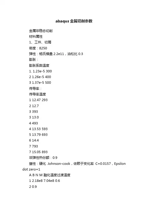
abaqus金属切削参数金属非稳态切削材料属性1、工件、切屑密度:8250弹性:杨氏模量2.2e11,泊松比0.3膨胀:膨胀系数温度1. 1.23e-5 3002 1.26e-5 4003 1.37e-5 500传导率:传导率温度1 12.47 2932 12.73 3933 13.04 4934 13.53 5935 13.79 6936 14.47 7937 15.05 893非弹性热份额:0.9塑性:硬化Johnson-cook,依赖于变化率C=0.0157,Epsilon dot zero=1A B N M 融化温度过渡温度1 2.18e8 7.04e8 0.62 0.93 850 300比热:2032、分离线剪切损伤:断裂应变2,损伤演化:破坏位移4e-63、刀具传导率:46质量密度:15000弹性:杨氏模量8e11,泊松比0.2膨胀:4.7e-6比热:20000截面属性均质实体,平面应力/应变厚度0.002分析步切削分析步:动力,温度-位移,显式时间长度:2.5e-5接触属性1、切向行为:粗糙;法向行为:不允许接触后分离;热传导2、切向行为:无摩擦;法向行为:允许接触后分离;热传导;生热:分布在从表面上的换热百分比0.9热传导:conductance clearance10000000 00 0.00013、切向行为:无摩擦;法向行为:允许接触后分离相互作用初始、表面与表面接触、接触属性1:切屑下&分离线上,工件上&分离线下(罚接触方法、有限滑移)切削、表面与表面接触、接触属性2:刀具&切屑下,工件上&切屑下(运动接触法、有限滑移)切削、自接触、接触属性3:切屑表面(运动接触法)幅度曲线时间/频率幅值1 0 02 2e-6 13 2.3e-5 14 2.5e-5 0进给速度:40温度场工件、切屑、分离线:300刀具:600网格网格控制属性:工件(四边形、结构);刀具(三角形、自由)单元类型:工件(CPE4RT: 四结点热耦合平面应变四边形单元, 双线性位移和温度, 减缩积分, 沙漏控制.);刀具(CPE3T: 三结点平面应变热耦合三角形单元, 位移和温度均线性.)金属稳态切削材料属性1、工件、切屑密度:7850弹性:杨氏模量2.08e11,泊松比0.3 膨胀:传导率:44.5非弹性热份额:0.9塑性:硬化Johnson-cook ,依赖于变化率C=0.014,Epsilon dot zero=1 比热:5022、刀具:解析刚体截面属性均质实体,平面应力/应变厚度1分析步初始分析步切削分析步:动力,显式时间长度:0.08接触属性切向行为:罚摩擦(各项同性摩擦系数0.4);法向行为相互作用切削分析步、表面与表面接触、接触属性:刀具&工件幅度曲线时间/频率幅值 1 0 0 2 0.001 1 3 0.079 1膨胀系数温度1. 1.23e-5 293 2 1.26e-5 523 3 1.37e-5773A B N M 融化温度过渡温度 1 1.15e9 7.39e8 0.26 1.03 1723 2984 0.08 0进给速度:1温度场工件、刀具:298网格网格控制属性:工件(四边形、结构)单元类型:工件(CPE4RT: 四结点热耦合平面应变四边形单元, 双线性位移和温度, 减缩积分, 沙漏控制.)。
19 ABAQUS用户材料子程序(UMAT)虽然ABAQUS为用户提供了大量的单元库和求解模型,使用户能够利用这些模型处理绝大多数的问题;但是现实世界毕竟十分复杂,ABAQUS不可能把所有可能出现的问题都包含进去。
所以ABAQUS提供了大量的用户子程序(User Subroutine)。
用户子程序允许用户在找不到合适模型的情况下自行定义符合自己问题的模型。
这些用户子程序涵盖了建模从载荷到单元的几乎各个部分。
ABAQUS为用户提供的这个接口,允许用户通过自定义的子程序定制ABAQUS,以实现特定的功能。
用户子程序具有以下的功能和特点:(1)如果ABAQUS的一些固有选项模型功能有限;用户子程序可以提高ABAQUS中这些选项的功能;(2)通常用户子程序是用FORTRAN语言的代码写成;(3)它可以以几种不同的方式包含在模型中;(4)由于它们没有存储在restart文件中,如果需要的话,可以在重新开始运行时修改它;(5)在某些情况下它可以利用ABAQUS允许的已有程序。
要在模型中包含用户子程序,可以利用ABAQUS执行程序,在abaqus执行程序中应用user选项指明包含这些子程序的FORTRAN源程序或者目标程序的名字。
提示:ABAQUS的输入文件除了可以通过ABAQUS/CAE的作业模块中提交运行外,还可以在ABAQUS Command窗口中输入ABAQUS执行程序直接运行:ABAQUS job=输入文件名 user=用户子程序的Fortran文件名ABAQUS/Standard和ABAQUS/Explicit都支持用户子程序功能,但是他们所支持的用户子程序种类不尽相同,读者在需要使用时请注意查询手册。
在接下来的最后两章里,我们将讨论两种常用的用户子程序——用户材料子程序和用户单元子程序。
本章将通过在ABAQUS/Standard中创建Johnson-Cook的材料模型,对编写Standard 的用户材料子程序UMAT进行一个简单介绍。
1.1.41 UMATUser subroutine to define a material's mechanical behavior.Product: Abaqus/StandardWarning: The use of this subroutine generally requires considerable expertise. Y ou arecautioned that the implementation of any realistic constitutive model requires extensivedevelopment and testing. Initial testing on a single-element model with prescribedtraction loading is strongly recommended.References“User-defined mechanical material behavior,” Section 26.7.1 of the Abaqus Analysis User's Guide“User-defined thermal material behavior,” Section 26.7.2 of the Abaqus Analysis User's Guide*USER MA TERIAL“S D V I N I,” Section 4.1.11 of the Abaqus V erification Guide“U M A T and U H Y P E R,” Section 4.1.21 of the Abaqus V erification GuideOv erv iewUser subroutine U M A T:can be used to define the mechanical constitutive behavior of a material;will be called at all material calculation points of elements for which the material definition includes auser-defined material behavior;can be used with any procedure that includes mechanical behavior;can use solution-dependent state variables;must update the stresses and solution-dependent state variables to their values at the end of theincrement for which it is called;must provide the material Jacobian matrix, , for the mechanical constitutive model;can be used in conjunction with user subroutine U S D F L D to redefine any field variables before they are passed in; andis described further in “User-defined mechanical material behavior,” Section 26.7.1 of the AbaqusAnalysis User's Guide.Storage of stress and strain componentsIn the stress and strain arrays and in the matrices D D S D D E, D D S D D T, and D R P L D E, direct components are stored first, followed by shear components. There are N D I direct and N S H R engineering shear components. The order of the components is defined in “Conventions,” Section 1.2.2 of the Abaqus Analysis User's Guide. Since the number of active stress and strain components varies between element types, the routine must be coded toprovide for all element types with which it will be used.Defining local orientationsIf a local orientation (“Orientations,” Section 2.2.5 of the Abaqus Analysis User's Guide) is used at the same point as user subroutine U M A T, the stress and strain components will be in the local orientation; and, in the case of finite-strain analysis, the basis system in which stress and strain components are stored rotates with the material.StabilityY ou should ensure that the integration scheme coded in this routine is stable—no direct provision is made to include a stability limit in the time stepping scheme based on the calculations in U M A T.Convergence rateD D S D DE and—for coupled temperature-displacement and coupled thermal-electrical-structural analyses—D D S D D T, D R P L D E, and D R P L D T must be defined accurately if rapid convergence of the overall Newton scheme is to be achieved. In most cases the accuracy of this definition is the most important factor governing the convergence rate. Since nonsymmetric equation solution is as much as four times as expensive as the corresponding symmetric system, if the constitutive Jacobian (D D S D D E) is only slightly nonsymmetric (for example, a frictional material with a small friction angle), it may be less expensive computationally to use a symmetric approximation and accept a slower convergence rate.An incorrect definition of the material Jacobian affects only the convergence rate; the results (if obtained) are unaffected.Special considerations for various element typesThere are several special considerations that need to be noted.A v ailability of deformation gradientThe deformation gradient is available for solid (continuum) elements, membranes, and finite-strain shells(S3/S3R, S4, S4R, SAXs, and SAXAs). It is not available for beams or small-strain shells. It is stored as a 3× 3 matrix with component equivalence D F G R D0(I,J). For fully integrated first-order isoparametric elements (4-node quadrilaterals in two dimensions and 8-node hexahedra in three dimensions) the selectively reduced integration technique is used (also known as the technique). Thus, a modified deformation gradientis passed into user subroutine U M A T. For more details, see “Solid isoparametric quadrilaterals and hexahedra,”Section 3.2.4 of the Abaqus Theory Guide.Beams and shells that calculate transv erse shear energyIf user subroutine U M A T is used to describe the material of beams or shells that calculate transverse shear energy, you must specify the transverse shear stiffness as part of the beam or shell section definition to define the transverse shear behavior. See “Shell section behavior,” Section 29.6.4 of the Abaqus Analysis User's Guide, and “Choosing a beam element,” Section 29.3.3 of the Abaqus Analysis User's Guide, for informationon specifying this stiffness.Open-section beam elementsWhen user subroutine U M A T is used to describe the material response of beams with open sections (for example, an I-section), the torsional stiffness is obtained aswhere J is the torsional constant, A is the section area, k is a shear factor, and is the user-specified transverse shear stiffness (see “Transverse shear stiffness definition” in “Choosing a beam element,” Section29.3.3 of the Abaqus Analysis User's Guide).E lements w ith hourglassing modesIf this capability is used to describe the material of elements with hourglassing modes, you must define the hourglass stiffness factor for hourglass control based on the total stiffness approach as part of the element section definition. The hourglass stiffness factor is not required for enhanced hourglass control, but you can define a scaling factor for the stiffness associated with the drill degree of freedom (rotation about the surface normal). See “Section controls,” Section 27.1.4 of the Abaqus Analysis User's Guide, for information on specifying the stiffness factor.Pipe-soil interaction elementsThe constitutive behavior of the pipe-soil interaction elements (see “Pipe-soil interaction elements,” Section 32.12.1 of the Abaqus Analysis User's Guide) is defined by the force per unit length caused by relative displacement between two edges of the element. The relative-displacements are available as “strains” (S T R A N and D S T R A N). The corresponding forces per unit length must be defined in the S T R E S S array. The Jacobian matrix defines the variation of force per unit length with respect to relative displacement.For two-dimensional elements two in-plane components of “stress” and “strain” exist (N T E N S=N D I=2, andN S H R=0). For three-dimensional elements three components of “stress” and “strain” exist (N T E N S=N D I=3, and N S H R=0).Large volume changes with geometric nonlinearityIf the material model allows large volume changes and geometric nonlinearity is considered, the exact definition of the consistent Jacobian should be used to ensure rapid convergence. These conditions are most commonly encountered when considering either large elastic strains or pressure-dependent plasticity. In the former case, total-form constitutive equations relating the Cauchy stress to the deformation gradient are commonly used; in the latter case, rate-form constitutive laws are generally used.For total-form constitutive laws, the exact consistent Jacobian is defined through the variation in Kirchhoff stress:Here, J is the determinant of the deformation gradient, is the Cauchy stress, is the virtual rate of deformation, and is the virtual spin tensor, defined asFor rate-form constitutive laws, the exact consistent Jacobian is given byUse with incompressible elastic materialsFor user-defined incompressible elastic materials, user subroutine U H Y P E R should be used rather than user subroutine U M A T. In U M A T incompressible materials must be modeled via a penalty method; that is, you must ensure that a finite bulk modulus is used. The bulk modulus should be large enough to model incompressibility sufficiently but small enough to avoid loss of precision. As a general guideline, the bulk modulus should be about – times the shear modulus. The tangent bulk modulus can be calculated fromIf a hybrid element is used with user subroutine U M A T, Abaqus/Standard will replace the pressure stress calculated from your definition of S T R E S S with that derived from the Lagrange multiplier and will modify the Jacobian appropriately.For incompressible pressure-sensitive materials the element choice is particularly important when using user subroutine U M A T. In particular, first-order wedge elements should be avoided. For these elements the technique is not used to alter the deformation gradient that is passed into user subroutine U M A T, which increases the risk of volumetric locking.Increments for which only the Jacobian can be definedAbaqus/Standard passes zero strain increments into user subroutine U M A T to start the first increment of all the steps and all increments of steps for which you have suppressed extrapolation (see “Defining an analysis,”Section 6.1.2 of the Abaqus Analysis User's Guide). In this case you can define only the Jacobian (D D S D D E).Utility routinesSeveral utility routines may help in coding user subroutine U M A T. Their functions include determining stress invariants for a stress tensor and calculating principal values and directions for stress or strain tensors. These utility routines are discussed in detail in “Obtaining stress invariants, principal stress/strain values and directions, and rotating tensors in an Abaqus/Standard analysis,” Section 2.1.11.U ser subroutine interfaceS U B R O U T I N E U M A T(S T R E S S,S T A T E V,D D S D D E,S S E,S P D,S C D,1R P L,D D S D D T,D R P L D E,D R P L D T,2S T R A N,D S T R A N,T I M E,D T I M E,T E M P,D T E M P,P R E D E F,D P R E D,C M N A M E,3N D I,N S H R,N T E N S,N S T A T V,P R O P S,N P R O P S,C O O R D S,D R O T,P N E W D T,4C E L E N T,D F G R D0,D F G R D1,N O E L,N P T,L A Y E R,K S P T,K S T E P,K I N C)CI N C L U D E'A B A_P A R A M.I N C'C H A R A C T E R*80C M N A M ED I ME N S I O N S T R E S S(N T E N S),S T A T E V(N S T A T V),1D D S D D E(N T E N S,N T E N S),D D S D D T(N T E N S),D R P L D E(N T E N S),2S T R A N(N T E N S),D S T R A N(N T E N S),T I M E(2),P R E D E F(1),D P R E D(1),3P R O P S(N P R O P S),C O O R D S(3),D R O T(3,3),D F G R D0(3,3),D F G R D1(3,3)user coding to define D D S D D E,S T R E S S,S T A T E V,S S E,S P D,S C Dand, if necessary,R P L,D D S D D T,D R P L D E,D R P L D T,P N E W D TR E T U R NE N DV ariables to be definedIn all situationsD D S D D E(N TE N S,N T E N S)Jacobian matrix of the constitutive model, , where are the stress increments and are the strain increments. D D S D D E(I,J) defines the change in the I th stress component at the end of the time increment caused by an infinitesimal perturbation of the J th component of the strain increment array.Unless you invoke the unsymmetric equation solution capability for the user-defined material,Abaqus/Standard will use only the symmetric part of D D S D D E. The symmetric part of the matrix iscalculated by taking one half the sum of the matrix and its transpose.S T R E S S(N T E N S)This array is passed in as the stress tensor at the beginning of the increment and must be updated in this routine to be the stress tensor at the end of the increment. If you specified initial stresses (“Initial conditions in Abaqus/Standard and Abaqus/Explicit,” Section 34.2.1 of the Abaqus Analysis User's Guide), this array will contain the initial stresses at the start of the analysis. The size of this array depends on the value of N T E N S as defined below. In finite-strain problems the stress tensor has already been rotated to account for rigid body motion in the increment before U M A T is called, so that only the corotational part of the stress integration should be done in U M A T. The measure of stress used is “true” (Cauchy) stress.S T A T E V(N S T A T V)An array containing the solution-dependent state variables. These are passed in as the values at thebeginning of the increment unless they are updated in user subroutines U S D F L D or U E X P A N, in which case the updated values are passed in. In all cases S T A T E V must be returned as the values at the end of the increment. The size of the array is defined as described in “Allocating space” in “User subroutines:overview,” Section 18.1.1 of the Abaqus Analysis User's Guide.In finite-strain problems any vector-valued or tensor-valued state variables must be rotated to account for rigid body motion of the material, in addition to any update in the values associated with constitutivebehavior. The rotation increment matrix, D R O T, is provided for this purpose.S S E,S P D,S C DSpecific elastic strain energy, plastic dissipation, and “creep” dissipation, respectively. These are passed in as the values at the start of the increment and should be updated to the corresponding specific energy values at the end of the increment. They have no effect on the solution, except that they are used forenergy output.Only in a fully coupled thermal-stress or a coupled thermal-electrical-structural analysisR P LV olumetric heat generation per unit time at the end of the increment caused by mechanical working of the material.D D S D D T(N TE N S)V ariation of the stress increments with respect to the temperature.D R P L D E(N TE N S)V ariation of R P L with respect to the strain increments.D R P L D TV ariation of R P L with respect to the temperature.Only in a geostatic stress procedure or a coupled pore fluid diffusion/stress analysis for pore pressure cohesive elementsR P LR P L is used to indicate whether or not a cohesive element is open to the tangential flow of pore fluid. Set R P L equal to 0 if there is no tangential flow; otherwise, assign a nonzero value to R P L if an element is open.Once opened, a cohesive element will remain open to the fluid flow.V ariable that can be updatedP N E W D TRatio of suggested new time increment to the time increment being used (D T I M E, see discussion later in this section). This variable allows you to provide input to the automatic time incrementation algorithms in Abaqus/Standard (if automatic time incrementation is chosen). For a quasi-static procedure the automatic time stepping that Abaqus/Standard uses, which is based on techniques for integrating standard creep laws (see “Quasi-static analysis,” Section 6.2.5 of the Abaqus Analysis User's Guide), cannot becontrolled from within the U M A T subroutine.P N E W D T is set to a large value before each call to U M A T.If P N E W D T is redefined to be less than 1.0, Abaqus/Standard must abandon the time increment andattempt it again with a smaller time increment. The suggested new time increment provided to theautomatic time integration algorithms is P N E W D T × D T I M E, where the P N E W D T used is the minimum value for all calls to user subroutines that allow redefinition of P N E W D T for this iteration.If P N E W D T is given a value that is greater than 1.0 for all calls to user subroutines for this iteration and the increment converges in this iteration, Abaqus/Standard may increase the time increment. The suggestednew time increment provided to the automatic time integration algorithms is P N E W D T × D T I M E, where the P N E W D T used is the minimum value for all calls to user subroutines for this iteration.If automatic time incrementation is not selected in the analysis procedure, values of P N E W D T that aregreater than 1.0 will be ignored and values of P N E W D T that are less than 1.0 will cause the job to terminate. V ariables passed in for informationS T R A N(N T E N S)An array containing the total strains at the beginning of the increment. If thermal expansion is included in the same material definition, the strains passed into U M A T are the mechanical strains only (that is, thethermal strains computed based upon the thermal expansion coefficient have been subtracted from the total strains). These strains are available for output as the “elastic” strains.In finite-strain problems the strain components have been rotated to account for rigid body motion in the increment before U M A T is called and are approximations to logarithmic strain.D S T R A N(N TE N S)Array of strain increments. If thermal expansion is included in the same material definition, these are the mechanical strain increments (the total strain increments minus the thermal strain increments).T I M E(1)V alue of step time at the beginning of the current increment or frequency.T I M E(2)V alue of total time at the beginning of the current increment.D T I M ETime increment.T E M PTemperature at the start of the increment.D TE M PIncrement of temperature.P R E D E FArray of interpolated values of predefined field variables at this point at the start of the increment, based on the values read in at the nodes.D P RE DArray of increments of predefined field variables.C M N A M EUser-defined material name, left justified. Some internal material models are given names starting with the “ABQ_” character string. To avoid conflict, you should not use “ABQ_” as the leading string for C M N A M E. N D INumber of direct stress components at this point.N S H RNumber of engineering shear stress components at this point.N T E N SSize of the stress or strain component array (N D I + N S H R).N S T A T VNumber of solution-dependent state variables that are associated with this material type (defined asdescribed in “Allocating space” in “User subroutines: overview,” Section 18.1.1 of the Abaqus Analysis User's Guide).P R O P S(N P R O P S)User-specified array of material constants associated with this user material.N P R O P SUser-defined number of material constants associated with this user material.C O O RD SAn array containing the coordinates of this point. These are the current coordinates if geometricnonlinearity is accounted for during the step (see “Defining an analysis,” Section 6.1.2 of the Abaqus Analysis User's Guide); otherwise, the array contains the original coordinates of the point.D R O T(3,3)Rotation increment matrix. This matrix represents the increment of rigid body rotation of the basis system in which the components of stress (S T R E S S) and strain (S T R A N) are stored. It is provided so that vector-or tensor-valued state variables can be rotated appropriately in this subroutine: stress and straincomponents are already rotated by this amount before U M A T is called. This matrix is passed in as a unit matrix for small-displacement analysis and for large-displacement analysis if the basis system for thematerial point rotates with the material (as in a shell element or when a local orientation is used).C E L E N TCharacteristic element length, which is a typical length of a line across an element for a first-order element;it is half of the same typical length for a second-order element. For beams and trusses it is a characteristic length along the element axis. For membranes and shells it is a characteristic length in the referencesurface. For axisymmetric elements it is a characteristic length in the plane only. For cohesiveelements it is equal to the constitutive thickness.D F G R D0(3,3)Array containing the deformation gradient at the beginning of the increment. If a local orientation is defined at the material point, the deformation gradient components are expressed in the local coordinate system defined by the orientation at the beginning of the increment. For a discussion regarding the availability of the deformation gradient for various element types, see “Availability of deformation gradient.”D F G R D1(3,3)Array containing the deformation gradient at the end of the increment. If a local orientation is defined at the material point, the deformation gradient components are expressed in the local coordinate system defined by the orientation. This array is set to the identity matrix if nonlinear geometric effects are not included in the step definition associated with this increment. For a discussion regarding the availability of thedeformation gradient for various element types, see “Availability of deformation gradient.”N O E LElement number.N P TIntegration point number.L A Y E RLayer number (for composite shells and layered solids).K S P TSection point number within the current layer.K S T E PStep number.K I N CIncrement number.Example: Using more than one user-defined mechanical material modelTo use more than one user-defined mechanical material model, the variable C M N A M E can be tested for different material names inside user subroutine U M A T as illustrated below:I F(C M N A M E(1:4).E Q.'M A T1')T H E NC A L L U M A T_M A T1(argument_list)E L S E I F(C M N A M E(1:4).E Q.'M A T2')T H E NC A L L U M A T_M A T2(argument_list)E N D I FU M A T_M A T1 and U M A T_M A T2 are the actual user material subroutines containing the constitutive material models for each material M A T1 and M A T2, respectively. Subroutine U M A T merely acts as a directory here. The argument list may be the same as that used in subroutine U M A T.Example: Simple linear viscoelastic materialAs a simple example of the coding of user subroutine U M A T, consider the linear, viscoelastic model shown in Figure 1.1.41–1. Although this is not a very useful model for real materials, it serves to illustrate how to code the routine.Figure 1.1.41–1 Simple linear viscoelastic model.The behavior of the one-dimensional model shown in the figure iswhere and are the time rates of change of stress and strain. This can be generalized for small straining of an isotropic solid asandwhereand , , , , and are material constants ( and are the Lamé constants).A simple, stable integration operator for this equation is the central difference operator:where f is some function, is its value at the beginning of the increment, is the change in the function over the increment, and is the time increment.Applying this to the rate constitutive equations above givesandso that the Jacobian matrix has the termsandThe total change in specific energy in an increment for this material iswhile the change in specific elastic strain energy iswhere D is the elasticity matrix:No state variables are needed for this material, so the allocation of space for them is not necessary. In a morerealistic case a set of parallel models of this type might be used, and the stress components in each model might be stored as state variables.For our simple case a user material definition can be used to read in the five constants in the order , , , , and so thatThe routine can then be coded as follows:S U B R O U T I N E U M A T(S T R E S S,S T A T E V,D D S D D E,S S E,S P D,S C D,1R P L,D D S D D T,D R P L D E,D R P L D T,2S T R A N,D S T R A N,T I M E,D T I M E,T E M P,D T E M P,P R E D E F,D P R E D,C M N A M E,3N D I,N S H R,N T E N S,N S T A T V,P R O P S,N P R O P S,C O O R D S,D R O T,P N E W D T,4C E L E N T,D F G R D0,D F G R D1,N O E L,N P T,L A Y E R,K S P T,K S T E P,K I N C)CI N C L U D E'A B A_P A R A M.I N C'CC H A R A C T E R*80C M N A M ED I ME N S I O N S T R E S S(N T E N S),S T A T E V(N S T A T V),1D D S D D E(N T E N S,N T E N S),2D D S D D T(N T E N S),D R P L D E(N T E N S),3S T R A N(N T E N S),D S T R A N(N T E N S),T I M E(2),P R E D E F(1),D P R E D(1),4P R O P S(N P R O P S),C O O R D S(3),D R O T(3,3),D F G R D0(3,3),D F G R D1(3,3)D I ME N S I O N D S T R E S(6),D(3,3)CC E V A L U A T E N E W S T R E S S T E N S O RCE V=0.D E V=0.D O K1=1,N D IE V=E V+S T R A N(K1)D E V=D E V+D S T R A N(K1)E N D D OCT E R M1=.5*D T I M E+P R O P S(5)T E R M1I=1./T E R M1T E R M2=(.5*D T I M E*P R O P S(1)+P R O P S(3))*T E R M1I*D E VT E R M3=(D T I M E*P R O P S(2)+2.*P R O P S(4))*T E R M1ICD O K1=1,N D ID S T RE S(K1)=T E R M2+T E R M3*D S T R A N(K1)1+D T I M E*T E R M1I*(P R O P S(1)*E V2+2.*P R O P S(2)*S T R A N(K1)-S T R E S S(K1))S T R E S S(K1)=S T R E S S(K1)+D S T R E S(K1)E N D D OCT E R M2=(.5*D T I M E*P R O P S(2)+P R O P S(4))*T E R M1II1=N D ID O K1=1,N S H RI1=I1+1D S T RE S(I1)=T E R M2*D S T R A N(I1)+1D T I M E*T E R M1I*(P R O P S(2)*S T R A N(I1)-S T R E S S(I1)) S T R E S S(I1)=S T R E S S(I1)+D S T R E S(I1)E N D D OCC C R E A T E N E W J A C O B I A NCT E R M2=(D T I M E*(.5*P R O P S(1)+P R O P S(2))+P R O P S(3)+12.*P R O P S(4))*T E R M1IT E R M3=(.5*D T I M E*P R O P S(1)+P R O P S(3))*T E R M1ID O K1=1,N TE N SD O K2=1,N TE N SD D S D D E(K2,K1)=0.E N D D OE N D D OCD O K1=1,N D ID D S D D E(K1,K1)=TE R M2E N D D OCD O K1=2,N D IN2=K1–1D O K2=1,N2D D S D D E(K2,K1)=TE R M3D D S D D E(K1,K2)=TE R M3E N D D OE N D D OT E R M2=(.5*D T I M E*P R O P S(2)+P R O P S(4))*T E R M1II1=N D ID O K1=1,N S H RI1=I1+1D D S D D E(I1,I1)=TE R M2E N D D OCC T O T A L C H A N G E I N S P E C I F I C E N E R G YCT D E=0.D O K1=1,N TE N ST D E=T D E+(S T R E S S(K1)-.5*D S T R E S(K1))*D S T R A N(K1)E N D D OCC C H A N G E I N S P E C I F I C E L A S T I C S T R A I N E N E R G YCT E R M1=P R O P S(1)+2.*P R O P S(2)D O K1=1,N D ID(K1,K1)=T E R M1E N D D OD O K1=2,N D IN2=K1-1D O K2=1,N2D(K1,K2)=P R O P S(1)D(K2,K1)=P R O P S(1)E N D D OE N D D OD E E=0.D O K1=1,N D IT E R M1=0.T E R M2=0.D O K2=1,N D IT E R M1=T E R M1+D(K1,K2)*S T R A N(K2)T E R M2=T E R M2+D(K1,K2)*D S T R A N(K2)E N D D OD E E=D E E+(T E R M1+.5*T E R M2)*D S T R A N(K1)E N D D OI1=N D ID O K1=1,N S H RI1=I1+1D E E=D E E+P R O P S(2)*(S T R A N(I1)+.5*D S T R A N(I1))*D S T R A N(I1)E N D D OS S E=S S E+D E ES C D=S C D+T D E– D E ER E T U R NE N D。

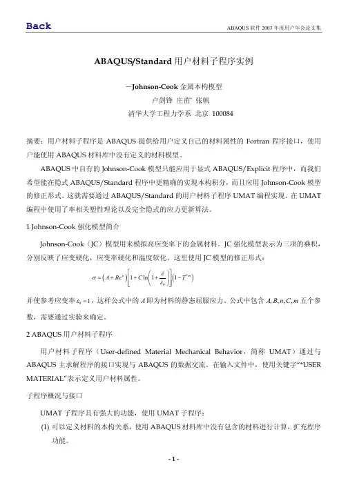
Johnson-Cook本构模型是一种在冲击动力学中应用广泛的模型,适用于模拟许多材料在高应变率下的变形。
这个模型考虑了流变应力、应变、应变速率和温度之间的关系,其公式简单明了。
该模型由三部分构成,分别表征了材料的应变硬化、应变速率强化以及热软化。
然而,这个模型采用简单的乘积形式将三项联立,这意味着它只是单独考虑了应变、应变速率和温度的影响,而并未考虑各因素之间的耦合影响。
因此,在某些特殊情况下,模型的精度可能会存在问题。
此外,Johnson-Cook塑性模型是一种具有硬化规律和速率依赖的解析形式的米塞斯塑性模型,主要适用于许多材料的高应变率变形模拟,包括大多数金属。
它通常用于绝热瞬态动态模拟,可以与Abaqus/Explicit中的Johnson-Cook动态失效模型结合使用。
在Abaqus/Explicit中,它可以结合拉伸破坏模型来模拟拉伸剥落或压力断口。
此外,它可以与渐进损伤和失效模型结合使用,以指定不同的损伤起始准则和损伤演化规律,同时允许材料刚度的渐进退化和网格单元的移除。
需要注意的是,必须与线弹性材料模型或状态方程材料模型结合使用。
总的来说,Johnson-Cook本构模型在模拟高应变率变形方面具有重要应用,但在使用时需要注意其局限性。
abaqus johnson cook失效准则Abaqus Johnson-Cook Failure Criterion: An In-depth AnalysisIntroduction:The Abaqus Johnson-Cook failure criterion is widely used in the field of computational modeling and simulation to predict material failure under extreme conditions. This criterion is paramount in accurately predicting how a material will deform and eventually fail under various loading conditions. In this article, we will provide a step-by-step analysis of the Abaqus Johnson-Cook failure criterion, its underlying principles, and its applications in engineering simulations.1. Background and Theory:The Johnson-Cook failure criterion was originally proposed by G.R. Johnson and W.H. Cook in 1983. It provides a phenomenological representation of the material behavior leading to failure under high strain rates and elevated temperatures. The criterion takes into account the effects of strain, strain rate, and temperature on the material's response to loading. By considering these factors, thefailure criterion allows for a more accurate prediction of material failure.2. Formulation of the Criterion:The Abaqus Johnson-Cook failure criterion can be mathematically represented as follows:σ_eq = (1 + αε˙_pl^* (T - T_0))^m (1 - β(T - T_0))^nwhere σ_eq is the equivalent stress, αand βare material constants, ε˙_pl^* is the plastic strain rate, T is the temperature, T_0 is a reference temperature, and m and n are exponent parameters. This equation describes the relationship between stress, strain rate, temperature, and material failure.3. Parameter Determination:To accurately define the material constants α, β, m, and n, experimental data is necessary. These constants are typically obtained through a series of experimental tests, such as tensile tests at different strain rates and temperatures. The results fromthese tests are then used to fit the parameters in the Johnson-Cook equation to obtain a reliable representation of the material behavior.4. Material Model Implementation:In Abaqus, the Johnson-Cook failure criterion is implemented through a specific material model. The material model incorporates the Johnson-Cook equation and provides a framework to simulate the behavior of materials subjected to high strain rates and elevated temperatures. The user must input the relevant material properties and the determined values for α, β, m, and n into the material model.5. Applications:The Abaqus Johnson-Cook failure criterion has found numerous applications across various engineering disciplines. It is particularly relevant in the fields of impact dynamics, projectile penetration, blast effects, and metal forming processes. By accurately predicting material failure, engineers can design structures and components with a higher level of safety and durability.6. Validation and Verification:Before utilizing the Abaqus Johnson-Cook failure criterion in engineering simulations, it is crucial to validate and verify the accuracy of the material model. This involves comparing the simulation results with experimental data obtained from laboratory tests. If the simulation results closely match the experimental results, it provides confidence in the predictive capability of the model.7. Advantages and Limitations:The Abaqus Johnson-Cook failure criterion allows engineers to simulate and predict material failure under extreme conditions, providing valuable insights for design and analysis purposes. However, it is important to note that the accuracy of the model heavily relies on accurate parameter determination and appropriate material model selection. Additionally, the criterion may not be suitable for all materials and certain scenarios, necessitating the use of alternative failure criteria.Conclusion:In conclusion, the Abaqus Johnson-Cook failure criterion is a valuable tool in predicting material failure under high strain rates and elevated temperatures. By considering the effects of strain, strain rate, and temperature in the material's response to loading, this criterion provides engineers with important insights during the design and analysis stages. However, it is crucial to accurately determine the material constants and validate the model to ensure reliable predictions. The Abaqus Johnson-Cook failure criterion continues to play a pivotal role in engineering simulations, contributing to safer and more efficient designs.。

abaqus 子程序简单案例1. 案例一:ABAQUS子程序在计算机辅助工程中的应用在计算机辅助工程中,ABAQUS子程序是一种被广泛应用的工具,用于求解各种复杂的物理问题。
它可以在ABAQUS有限元软件中调用,通过编写用户自定义的子程序来实现特定的功能。
下面将介绍一些常见的ABAQUS子程序案例。
2. 案例二:ABAQUS子程序在材料力学中的应用ABAQUS子程序在材料力学中的应用非常广泛。
例如,可以通过自定义的子程序来模拟材料的非线性行为、塑性变形、断裂行为等。
通过在子程序中编写相应的材料本构模型和损伤模型,可以准确地预测材料的力学性能。
3. 案例三:ABAQUS子程序在流体力学中的应用ABAQUS子程序在流体力学中也有重要的应用。
例如,可以通过自定义的子程序来模拟流体的非牛顿性、多相流动、湍流等现象。
通过在子程序中编写相应的流体本构模型和湍流模型,可以准确地模拟流体的流动行为。
4. 案例四:ABAQUS子程序在结构力学中的应用ABAQUS子程序在结构力学中也非常有用。
例如,可以通过自定义的子程序来模拟结构的非线性行为、接触和摩擦、动力响应等。
通过在子程序中编写相应的结构本构模型和接触模型,可以准确地预测结构的力学性能。
5. 案例五:ABAQUS子程序在热传导中的应用ABAQUS子程序在热传导中的应用也非常广泛。
例如,可以通过自定义的子程序来模拟材料的热传导行为、热辐射、相变等。
通过在子程序中编写相应的热传导模型和相变模型,可以准确地预测材料的热学性能。
6. 案例六:ABAQUS子程序在电磁场中的应用ABAQUS子程序在电磁场中的应用也有一定的研究价值。
例如,可以通过自定义的子程序来模拟电磁场的非线性行为、磁饱和、电磁感应等。
通过在子程序中编写相应的电磁场模型和电磁感应模型,可以准确地模拟电磁场的行为。
7. 案例七:ABAQUS子程序在声学中的应用ABAQUS子程序在声学领域中也有一定的应用。

abaqus中johnson-cook本构模型理解-回复Abaqus中Johnson-Cook本构模型理解引言:材料的本构模型是描述材料力学行为的数学方程。
在有限元分析中,本构模型可以用于模拟材料的变形和损伤行为,从而预测材料在不同加载条件下的响应。
Johnson-Cook本构模型是一种常用的本构模型,广泛应用于材料科学和工程领域。
本文将从基本原理开始,逐步解释和理解Abaqus 中Johnson-Cook本构模型。
1. 弹塑性本构模型首先需要了解的是,弹塑性本构模型是最基本的材料模型之一。
它基于线弹性理论,假设材料在小应变范围内具有弹性行为,而在大应变范围内表现出塑性行为。
弹塑性本构模型可以描述材料的应力-应变关系,并预测材料的弹性变形和塑性变形。
2. 材料的温度效应在考虑Johnson-Cook本构模型之前,还需要考虑材料的温度效应。
温度对材料力学行为的影响是复杂而重要的。
温度的增加可以引起材料的软化、蠕变和断裂等现象。
因此,在模拟材料行为时,必须考虑材料的温度效应,并选择适当的本构模型来描述。
3. Johnson-Cook本构模型的基本原理Johnson-Cook本构模型是一种经验模型,用于描述材料的塑性行为和温度效应。
它采用以下形式的应力-应变关系:σ= (A + B ε^n) (1 + C ln(ε˙/ε˙_0))^m (1 - T/T_m)^p其中,σ是材料的应力,ε是应变,ε˙是应变速率,T是材料的温度,A、B、C、n、m、p和T_m是需要通过实验来确定的材料参数。
4. 材料参数的确定为了使用Johnson-Cook本构模型,需要通过实验来确定材料参数。
这些参数通常由材料的拉伸实验和冲击实验等得到。
拉伸实验可以提供材料的应力-应变曲线,以及材料的屈服强度和断裂应变等信息。
冲击实验可以提供材料的应变率敏感性和断裂韧性等信息。
根据实验数据,可以使用不同的方法来确定Johnson-Cook本构模型的参数。

abaqus中johnson-cook本构模型理解-回复什么是Johnson-Cook本构模型?Johnson-Cook本构模型是一种经验性本构模型,用于描述金属材料在高速冲击、爆炸、高温和高应变率等极端条件下的力学行为。
它是由Johnson、Cook和Mackenzie等人于1983年提出的,并在后续的研究中进行了改进和发展。
Johnson-Cook本构模型已广泛应用于工程领域,尤其在汽车碰撞、航空航天以及防卫等领域中。
Johnson-Cook模型的核心思想是将材料的流变行为与材料的动力学参数相联系,从而描述材料在极端条件下的力学响应。
该模型基于一系列有效的材料试验数据,并引入了一些物理参数,以实现更准确的预测。
下面将详细介绍Johnson-Cook本构模型的具体形式以及其各个参数的含义:1. 应变率项:Johnson-Cook模型中的应变率项描述了材料在高应变率条件下的变形行为。
该项通常采用一般性的动力学方程,其中引入材料的应变硬化参数(A)、热软化参数(B)和应变率硬化指数(n)。
2. 温度项:Johnson-Cook模型中的温度项描述了材料在高温条件下的变形行为。
该项通常采用Arrhenius方程来表示材料的温度依赖性。
在此项中,引入材料的活化能(Q)、材料的平均绝对温度(T)和一些温度相关的材料常数。
3. 存在塑性起始的切应力项:Johnson-Cook模型中的切应力项描述了材料在塑性变形开始时所需的应力水平。
通过引入材料的初始应力(σ_0),可以实现对材料塑性变形起点的准确描述。
4. 塑性变形表征的切应变项:Johnson-Cook模型中的切应变项描述了材料的塑性变形行为。
该项通常采用一般性的功率方程,其中引入了材料的切应变硬化参数(C)和切应变硬化指数(m)。
5. 材料非均匀性描述的尺寸因子项:Johnson-Cook模型中的尺寸因子项用于考虑材料在非均匀加载条件下的力学响应。
在此项中,引入了材料的尺寸因子(δ)和一些与材料非均匀应变有关的参数。
1.1.37 UMATHTUser subroutine to define a material's thermalbehavior.Product: Abaqus/StandardWarning: The use of this subroutine generally requires considerable expertise. You are cautioned that the implementation of any realistic thermal model requires significant development and testing. Initial testing on models with few elements under a variety of boundary conditions is strongly recommended.References●“User-defined thermal material behavior,”Section 23.8.2 of the Abaqus Analysis User's Manual● *USER MATERIAL●“Freezing of a square solid: the two-dimensional Stefan problem,”Section 1.6.2 of the Abaqus Benchmarks Manual●“UMATHT,”Section 4.1.22 of the Abaqus Verification ManualOverviewUser subroutine UMATHT:● can be used to define the thermal constitutive behavior of the material as well as internal heat generation during heat transfer processes;● will be called at all material calculation points of elements for which the material definition includes a user-defined thermal material behavior;● can be used with the procedures discussed in “Heat transfer analysis procedures: overview,”Section 6.5.1 of the Abaqus Analysis User's Manual;● can use solution-dependent state Variables;● must define the internal energy per unit mass and its variation with respect to temperature and to spatial gradients of temperature;● must define the heat flux vector and its variation with respect to temperature and to gradients of temperature;● must update the solution-dependent state Variables to their values at the end of the increment;● can be used in conjunction with user subroutine USDFLD to redefine any field Variables before they are passed in; and● is described further in “User-defined thermal material behavior,”Section 23.8.2 of the Abaqus Analysis User's Manual.Use of subroutine UMATHT with coupled temperature-displacement elementsUser subroutine UMATHT should be used only with reduced-integration or modified coupled temperature-displacement elements if the mechanical and thermal fields are not coupled through plastic dissipation. No such restriction exists with fully integrated coupled temperature-displacement elements.User subroutine interfaceSUBROUTINE UMATHT(U,DUDT,DUDG,FLUX,DFDT,DFDG,1 STATEV,TEMP,DTEMP,DTEMDX,time,Dtime,PREDEF,DPRED,2 CMNAME,NTGRD,NSTATV,PROPS,NPROPS,COORDS,PNEWDT,3 NOEL,NPT,LAYER,KSPT,KSTEP,KINC)CINCLUDE 'ABA_PARAM.INC'CCHARACTER*80 CMNAMEDIMENSION DUDG(NTGRD),FLUX(NTGRD),DFDT(NTGRD),1 DFDG(NTGRD,NTGRD),STATEV(NSTATV),DTEMDX(NTGRD),2 time(2),PREDEF(1),DPRED(1),PROPS(NPROPS),COORDS(3)user coding to define U,DUDT,DUDG,FLUX,DFDT,DFDG,and possibly update STATEV, PNEWDTRETURNENDVariables to be definedUInternal thermal energy per unit mass, U, at the end of increment. This variable is passed in as the value at the start of the increment and must be updated to its value at the end of the increment.DUDTVariation of internal thermal energy per unit mass with respect to temperature,, evaluated at the end of the increment.DUDG(NTGRD)Variation of internal thermal energy per unit mass with respect to the spatial gradients of temperature,, at the end of the increment. The size of this array depends on the value of NTGRD as defined below. This term is typically zero in classical heat transfer analysis.FLUX(NTGRD)Heat flux vector,, at the end of the increment. This variable is passed in with the values at the beginning of the increment and must be updated to the values at the end of the increment.DFDT(NTGRD)Variation of the heat flux vector with respect to temperature,, evaluated at the end of the increment.DFDG(NTGRD,NTGRD)Variation of the heat flux vector with respect to the spatial gradients of temperature,, at the end of the increment. The size of this array depends on the value of NTGRD as defined below.Variables that can be updatedSTATEV(NSTATV)An array containing the solution-dependent state Variables.In an uncoupled heat transfer analysis STATEV is passedinto UMATHT with the values of these Variables at the beginning of the increment. However, any changes in STATEV made in usersubroutine USDFLD will be included in the values passed into UMATHT, since USDFLD is called before UMATHT. In addition, if UMATHT is being used in a fully coupled temperature-displacement analysis and user subroutine CREEP, user subroutine UEXPAN, user subroutine UMAT, or user subroutine UTRS is used to define the mechanical behavior of the material, those routines are called before this routine; therefore, any updating of STATEV done in CREEP, UEXPAN, UMAT, or UTRS will be included in the values passed into UMATHT.In all cases STATEV should be passed back from UMATHT as the values of the state Variables at the end of the current increment.PNEWDTratio of suggested new time increment to the time increment being used (DTIME, see below). This variable allows you to provide input to the automatic time incrementation algorithms in Abaqus/Standard (if automatic time incrementation is chosen).PNEWDT is set to a large value before each call to UMATHT.If PNEWDT is redefined to be less than 1.0, Abaqus/Standard must abandon the time increment and attempt it again with a smaller time increment. The suggested new time increment provided to the automatic time integration algorithms is PNEWDT ×DTIME, wherethe PNEWDT used is the minimum value for all calls to user subroutines that allow redefinition of PNEWDT for this iteration.If PNEWDT is given a value that is greater than 1.0 for all calls to user subroutines for this iteration and the increment converges in this iteration, Abaqus/Standard may increase the time increment. The suggested new time increment provided to the automatic time integration algorithms is PNEWDT ×DTIME, where the PNEWDT used is the minimum value for all calls to user subroutines for this iteration.If automatic time incrementation is not selected in the analysis procedure, values of PNEWDT that are greater than 1.0 will be ignored and values of PNEWDT that are less than 1.0 will cause the job to terminate.Variables passed in for informationTEMPTemperature at the start of the increment.DTEMPIncrement of temperature.DTEMDX(NTGRD)Current values of the spatial gradients of temperature,TIME(1)Value of step time at the beginning of the current increment.time(2)Value of total time at the beginning of the current increment.DTIMETime increment.PREDEFarray of interpolated values of predefined field Variables at this point at the start of the increment, based on the values read in at the nodes.DPREDarray of increments of predefined field Variables.CMNAMEUser-defined material name, left justified.NTGRDnumber of spatial gradients of temperature.NSTATVnumber of solution-dependent state variables associated with this material type (defined as described in “Allocating space” in “Usersubroutines: overview,”Section 15.1.1 of the Abaqus Analysis User's Manual).PROPS(NPROPS)User-specified array of material constants associated with this user material.NPROPSUser-defined number of material constants associated with this user material.COORDSAn array containing the coordinates of this point. These are the current coordinates in a fully coupled temperature-displacement analysis if geometric nonlinearity is accounted for during the step(see “Procedures: overview,”Section 6.1.1 of the Abaqus Analysis User's Manual); otherwise, the array contains the original coordinates of the point.NOEL :Element number.NPT :Integration point number.LAYER :Layer number (for composite shells and layered solids).KSPT: Section point number within the current layer.KSTEP: Step number.KINC: Increment number.Example: Using more than one user-defined thermal material modelTo use more than one user-defined thermal material model, the variable CMNAME can be tested for different material names inside user subroutine UMATHT, as illustrated below:IF (CMNAME(1:4) .EQ. 'MAT1') THENCALL UMATHT_MAT1(argument_list)ELSE IF(CMNAME(1:4) .EQ. 'MAT2') THENCALL UMATHT_MAT2(argument_list)END IFUMATHT_MAT1 and UMATHT_MAT2 are the actual user material subroutines containing the constitutive material models for each material MAT1 and MAT2, respectively. Subroutine UMATHT merely acts as a directory here. The argument list can be the same as that used in subroutine UMATHT.Example: Uncoupled heat transferAs a simple example of the coding of user subroutine UMATHT, consider uncoupled heat transfer analysis in a material. The equationsfor this case are developed here, and the corresponding UMATHT is given. This problem can also be solved by specifying thermal conductivity, specific heat, density, and internal heat generation directly.First, the equations for an uncoupled heat transfer analysis are outlined.The basic energy balance iswhere V is the volume of solid material with surface area S,is the density of the material,is the material time rate of the internal thermal energy, q is the heat flux per unit area of the body flowing into the body, and r is the heat supplied externally into the body per unit volume.A heat flux vectoris defined such thatwhereis the unit outward normal to the surface S. Introducing the above relation into the energy balance equation and using the divergence theorem, the following relation is obtained:The corresponding weak form is given bywhereis the temperature gradient andis an arbitrary variational field satisfying the essential boundary conditions.Introducing the backward difference integration algorithm:the weak form of the energy balance equation becomesThis nonlinear system is solved using Newton's method.In the above equations the thermal constitutive behavior of the material is given byAndwhereare state Variables.The Jacobian for Newton's method is given by (after dropping the subscriptson U)The thermal constitutive behavior for this example is now defined. We assume a constant specific heat for the material. The heat conduction in the material is assumed to be governed by Fourier's law.The internal thermal energy per unit mass is defined aswithwhere c is the specific heat of the material andFourier's law for heat conduction is given aswhereis the thermal conductivity matrix andis position, so thatandThe assumption of conductivity without any temperature dependence implies thatNo state variables are needed for this material, so the allocation of space for them is not necessary.A thermal user material definition can be used to read in the two constants for our simple case, namely the specific heat, c, and the coefficient of thermal conductivity, k, so thatSUBROUTINE UMATHT(U,DUDT,DUDG,FLUX,DFDT,DFDG,1 STATEV,TEMP,DTEMP,DTEMDX,time,DTIME,PREDEF,DPRED,2 CMNAME,NTGRD,NSTATV,PROPS,NPROPS,COORDS,PNEWDT,3 NOEL,NPT,LAYER,KSPT,KSTEP,KINC)CINCLUDE 'ABA_PARAM.INC'CCHARACTER*80 CMNAMEDIMENSION DUDG(NTGRD),FLUX(NTGRD),DFDT(NTGRD),1 DFDG(NTGRD,NTGRD),STATEV(NSTATV),DTEMDX(NTGRD),2 TIME(2),PREDEF(1),DPRED(1),PROPS(NPROPS),COORDS(3) CCOND = PROPS(1)SPECHT = PROPS(2)CDUDT = SPECHTDU = DUDT*DTEMPU = U+DUCDO I=1, NTGRDFLUX(I) = –COND*DTEMDX(I)DFDG(I,I) = –CONDEND DOCRETURNEND1.1.13 HETVALUser subroutine to provide internal heat generation in heat transfer analysis.Product: Abaqus/StandardReferences●“Uncoupled heat transfer analysis,”Section 6.5.2 of the Abaqus Analysis User's Manual●“Fully coupled thermal-stress analysis,”Section 6.5.4 of the Abaqus Analysis User's Manual● *HEAT GENERATION●“HETVAL,”Section 4.1.9 of the Abaqus Verification Manual OverviewUser subroutine HETVAL:● can be used to define a heat flux due to internal heatgeneration in a material, for example, as might be associated with phase changes occurring during the solution;● allows for the dependence of internal heat generation on state Variables (such as the fraction of material transformed) that themselves evolve with the solution and are stored as solution-dependent state variables;● will be called at all material calculation points for which the material definition contains volumetric heat generation during heat transfer, coupled temperature-displacement, or coupled thermal-electrical analysis procedures;● can be useful if it is necessary to include a kinetic theory fora phase change associated with latent heat release (for example, in the prediction of crystallization in a polymer casting process);● can be used in conjunction with user subroutine USDFLD if itis desired to redefine any field Variables before they are passed in; and● cannot be used with user subroutine UMATHT.User subroutine interfaceSUBROUTINE HETVAL(CMNAME,TEMP,time,DTIME,STATEV,FLUX,1 PREDEF,DPRED)CINCLUDE 'ABA_PARAM.INC'CCHARACTER*80 CMNAMECDIMENSION TEMP(2),STATEV(*),PREDEF(*),TIME(2),FLUX(2),1 DPRED(*)user coding to define FLUX and update STATEVRETURNENDVariables to be definedFLUX(1)Heat flux, r (thermal energy per time per volume: JT–1L–3), at this material calculation point.。
21 ABAQUS用户材料子程序(UMAT)虽然ABAQUS为用户提供了大量的单元库和求解模型,使用户能够利用这些模型处理绝大多数的问题;但是实际问题毕竟非常复杂,ABAQUS不可能直接求解所有可能出现的问题。
所以ABAQUS提供了大量的用户自定义子程序(User Subroutine),允许用户在找不到合适模型的情况下自行定义符合自己问题的模型。
这些用户子程序涵盖了建模、载荷到单元的几乎各个部分。
用户子程序具有以下的功能和特点:(1)如果ABAQUS的一些固有选项模型功能有限,用户子程序可以提高ABAQUS中这些选项的功能;(2)通常用户子程序是用FORTRAN语言的代码写成;(3)它可以以几种不同的方式包含在模型中;(4)由于它们没有存储在restart文件中,如果需要的话,可以在重新开始运行时修改它;(5)在某些情况下它可以利用ABAQUS允许的已有程序。
要在模型中包含用户子程序,可以利用ABAQUS执行程序,在执行程序中应用user 选项指明包含这些子程序的FORTRAN源程序或者目标程序的名字。
提示:ABAQUS的输入文件除了可以通过ABAQUS/CAE的作业模块中提交运行外,还可以在ABAQUS Command窗口中输入ABAQUS执行程序直接运行:ABAQUS job=输入文件名 user=用户子程序的Fortran文件名ABAQUS/Standard和ABAQUS/Explicit都支持用户子程序功能,但是他们所支持的用户子程序种类不尽相同,读者在需要使用时请注意查询手册。
在接下来的两章里,我们将讨论两种常用的用户子程序——用户材料子程序和用户单元子程序。
本章将通过在ABAQUS/Standard中创建Johnson-Cook的材料模型,介绍编写ABAQUS/Standard的用户材料子程序UMAT。
在ABAQUS/Explicit中编写用户材料子程序VUMAT与之相似,但是由于隐式和显式两种方法本身的差异,它们之间也有一些不同,请读者在具体使用前仔细查阅ABAQUS手册中的相关内容。
ABAQUS用户材料子程序开发及应用ABAQUS用户材料子程序开发及应用摘要:本文介绍了ABAQUS用户材料子程序的开发与应用。
首先,简要介绍了ABAQUS软件及其在工程领域的广泛应用。
然后,详细阐述了用户材料子程序的概念及作用,并介绍了子程序的开发流程和必要步骤。
接着,以一个具体的材料模型开发为例,详细介绍了子程序的实现方法和注意事项。
最后,以轴对称挤压模拟为例,展示了用户材料子程序在实际工程分析中的应用,并讨论了其优点和局限性。
关键词:ABAQUS;用户材料子程序;开发;应用一、引言ABAQUS是一款广泛应用于工程领域的有限元分析软件。
其强大的建模和分析能力使得工程师可以准确地模拟和分析各种结构和材料的行为。
然而,对于一些非标准材料或特殊材料,ABAQUS自带的材料模型可能无法满足工程师的需求。
此时,用户材料子程序的开发就显得尤为重要。
二、用户材料子程序的概念及作用用户材料子程序是指由ABAQUS用户自行编写的用于描述非标准材料行为的子程序。
它可以根据特定的材料性质和应变-应力关系,定义材料模型的行为,并将其与ABAQUS的有限元分析过程相结合。
通过用户材料子程序,工程师可以更加准确地模拟和分析特殊材料的行为,提高分析结果的可靠性和准确性。
三、用户材料子程序的开发流程和步骤用户材料子程序的开发包括以下几个基本步骤:1. 确定材料模型:根据实际需要和具体材料的性质,选择合适的材料模型。
常见的模型包括线弹性模型、塑性模型、粘弹性模型等。
2. 编写用户材料子程序:使用合适的编程语言(如Fortran)编写用户材料子程序,实现材料模型的行为。
子程序应包括材料刚度矩阵计算、应力和塑性应变更新等关键计算部分。
3. 软件接口设置:将编写好的用户材料子程序与ABAQUS 软件进行接口设置,以实现子程序与有限元分析的集成。
4. 验证与调试:使用合适的测试用例对子程序进行验证和调试,确保其计算结果与实际情况吻合。
A B A Q U S用户子程序(总4页)本页仅作为文档封面,使用时可以删除This document is for reference only-rar21year.MarchABAQUS用户子程序ABAQUS/Standard subroutines:: Define time-dependent, viscoplastic behavior (creep and swelling).定义和时间相关的、粘塑性的运动(蠕变和膨胀)2. DFLOW: Define nonuniform pore fluid velocity in a consolidation analysis.在压实分析中,定义非均匀孔隙流速度3. DFLUX: Define nonuniform distributed flux in a heat transfer or mass diffusion analysis.在热传递和质量扩散分析中,定义非均匀的分布流量4. DISP: Specify prescribed boundary conditions.指定规定的边界条件5. DLOAD: Specify nonuniform distributed loads.指定非均匀的分布荷载6. FILM: Define nonuniform film coefficient and associated sink temperatures for heattransfer analysis.对热传递分析指定非均匀的膜层散热系数和联合的散热器温度7. FLOW: Define nonuniform seepage coefficient and associated sink pore pressure for consolidation analysis.对压实分析定义非均匀的渗流系数和渗入孔隙压力8. FRIC: Define frictional behavior for contact surfaces.对接触面定义摩擦9. GAPCON: Define conductance between contact surfaces or nodes in a fully coupled temperature-displacement analysis or pure heat transfer analysis.在一个完全耦合的温度—置换分析或者是纯热传递分析中,定义接触面或节点间的导热系数。
(完整)ABAQUS金属切削实例步骤编辑整理:尊敬的读者朋友们:这里是精品文档编辑中心,本文档内容是由我和我的同事精心编辑整理后发布的,发布之前我们对文中内容进行仔细校对,但是难免会有疏漏的地方,但是任然希望((完整)ABAQUS金属切削实例步骤)的内容能够给您的工作和学习带来便利。
同时也真诚的希望收到您的建议和反馈,这将是我们进步的源泉,前进的动力。
本文可编辑可修改,如果觉得对您有帮助请收藏以便随时查阅,最后祝您生活愉快业绩进步,以下为(完整)ABAQUS金属切削实例步骤的全部内容。
背景介绍:切削过程是一个很复杂的工艺过程,它不但涉及到弹性力学、塑性力学、断裂力学,还有热力学、摩擦学等。
同时切削质量受到刀具形状、切屑流动、温度分布、热流和刀具磨损等影响,切削表面的残余应力和残余应变严重影响了工件的精度和疲劳寿命。
利用传统的解析方法,很难对切削机理进行定量的分析和研究。
计算机技术的飞速发展使得利用有限元仿真方法来研究切削加工过程以及各种参数之间的关系成为可能。
近年来,有限元方法在切削工艺中的应用表明,切削工艺和切屑形成的有限元模拟对了解切削机理,提高切削质量是很有帮助的。
这种有限元仿真方法适合于分析弹塑性大变形问题,包括分析与温度相关的材料性能参数和很大的应变速率问题.ABAQUS作为有限元的通用软件,在处理这种高度非线性问题上体现了它独到的优势,目前国际上对切削问题的研究大都采用此软件,因此,下面针对ABAQUS的切削做一个入门的例子,希望初学者能够尽快入门,当然要把切削做好,不单单是一个例子能够解决问题的,随着深入的研究,你会发现有很多因素影响切削的仿真的顺利进行,这个需要自己去不断探索,在此本人权当抛砖引玉,希望各位切削的大神们能够积极探讨起来,让我们在切削仿真的探索上更加精确,更加完善.~~~~~~~~~~~~~~~~~~~~~~~~~~~~~~~~~~~~~~~~~~~~~~~~~~~~~~~~~~~~~~~~~~~~~~~~~~~~~~~~~~~~~~~~~~~~~~~~~~~~~~~切削参数:切削速度300m/min,切削厚度0.1mm,切削宽度1mm尺寸参数:本例作为入门例子,为了简化问题,假定刀具为解析刚体,因为在切削过程中,一般我们更注重工件最终的切削质量,如应力场,温度场等,尤其是残余应力场,而如果是要进行刀具磨损或者涂层刀具失效的分析的话,那就要考虑建立刀具为变形体来进行分析了。
ABAQUS有限元程序中Jonson-Cook断裂准则与原始模型的差异及对比分析肖新科; 王要沛【期刊名称】《《南阳理工学院学报》》【年(卷),期】2018(010)006【摘要】Johnson-Cook断裂准则包含了应力三轴度、应变率和温度对材料延性的影响,广泛应用于金属材料在高应变率下断裂行为的预测,如爆炸冲击和切削。
但是ABAQUS中Johnson-Cook断裂准则(J-C-A)的表达式与原始Johnson-Cook 断裂准则(J-C)有差别,在ABAQUS中输入按J-C准则标定的模型参数时便会得到错误的材料断裂性能。
不幸的是,部分研究者没注意到这个差别。
将J-C断裂准则与J-C-A断裂准则进行了对比,并以Weldox 460 E钢的失效应变为例,展示了J-C 的预报效果以及采用J-C模型参数的J-C-A准则的预报效果。
最后,以公开文献中的一篇错误应用报道为例,详细说明了错误输入模型参数的预报效果。
【总页数】5页(P38-42)【作者】肖新科; 王要沛【作者单位】南阳理工学院土木工程学院河南南阳473004; 南阳理工学院软件学院河南南阳473004【正文语种】中文【中图分类】O385; TJ012.4【相关文献】1.应用ABAQUS有限元程序建立锚具试件分析模型 [J], 冯蕾2.基于ABAQUS的钢筋混凝土结构本构模型对比分析 [J], 孟闻远;王俊锋;张蕊;3.基于韧性断裂准则的修正MK模型及其在充液热成形中的应用 [J], 杨希英;郎利辉;刘康宁;郭禅4.ABAQUS软件本构模型中屈服准则的参数研究 [J], 董林伟;张明义;解云芸;李猛猛;徐建兴;陈兰霞5.基于ABAQUS的钢筋混凝土结构本构模型对比分析 [J], 孟闻远; 王俊锋; 张蕊因版权原因,仅展示原文概要,查看原文内容请购买。