Simulink入门指南
- 格式:pdf
- 大小:437.29 KB
- 文档页数:44

Simulink动态系统仿真入门Simulink是基于MA TLAB的图形化仿真设计环境,是MATLAB 提供的进行动态系统建模、仿真和综合分析的集成软件包。
它使用图形化的系统模块对动态系统进行描述,并在此基础上采用MATLAB 的计算引擎对动态系统在时域内进行求解。
它可以处理的系统包括:线性、非线性、离散、连续及混合、单任务、多任务离散事件等。
在MATLAB7.X版本中,可以直接在Simulink环境中运作的工具箱和模型库很多,已经覆盖了航天、航空、通信、控制、信号处理等等诸多领域,涉及内容专业性很强。
1、Simulink系统的启动由于Simulink和MATLAB是高度集成在一起的,因此启动Simulink必须先启动MA TLAB。
在MA TLAB启动Simulink可以通过在命令窗口输入Simulink,或者点击MATLAB工具栏的Simulink 快速启动图标。
启动Simulink后,出现Simulink的主窗口,选择主菜单File中的New\model,即可以打开系统模型编辑器。
下图依次是MATLAB 主窗口、Simulink主窗口和系统模型编辑窗口,图中的箭头表示了操作顺序。
在打开一个新的系统模型文件以后,用户可以从Simulink模块库中选择适合的系统模块或自定义模块来建立系统模型。
我们通过一个简单的例子来分步说明Simulink建模和仿真的能力。
1)在MATLAB 窗口运行Simulink。
打开Simulink模块库浏览器。
2)点击Source子库前的“+”展开库,可以看到各种信源模块。
3)点击新建图标,打开一个空白型的模型窗口。
4)用鼠标选中需要的信源模块,把它拖入新建的空白模型编辑窗口,生成一个正弦波的复制品。
5)同样将信宿库Sinks中的示波器Scope拷贝到模型窗口。
6)利用鼠标完成两个模块的连线操作,完成一个简单的模型。
7)为进行仿真,双击示波器模块,打开示波器显示屏。
Simulink仿真环境基础学习Simulink是面向框图的仿真软件。
7.1演示一个Simulink的简单程序【例7.1】创建一个正弦信号的仿真模型。
步骤如下:(1) 在MATLAB的命令窗口运行simulink命令,或单击工具栏中的图标,就可以打开Simulink模块库浏览器(Simulink Library Browser) 窗口,如图7.1所示。
图7.1 Simulink界面(2) 单击工具栏上的图标或选择菜单“File”——“New”——“Model”,新建一个名为“untitled”的空白模型窗口。
(3) 在上图的右侧子模块窗口中,单击“Source”子模块库前的“+”(或双击Source),或者直接在左侧模块和工具箱栏单击Simulink下的Source子模块库,便可看到各种输入源模块。
(4) 用鼠标单击所需要的输入信号源模块“Sine Wave”(正弦信号),将其拖放到的空白模型窗口“untitled”,则“Sine Wave”模块就被添加到untitled窗口;也可以用鼠标选中“Sine Wave”模块,单击鼠标右键,在快捷菜单中选择“add to 'untitled'”命令,就可以将“Sine Wave”模块添加到untitled窗口,如图7.2所示。
(5) 用同样的方法打开接收模块库“Sinks”,选择其中的“Scope”模块(示波器)拖放到“untitled”窗口中。
(6) 在“untitled”窗口中,用鼠标指向“Sine Wave”右侧的输出端,当光标变为十字符时,按住鼠标拖向“Scope”模块的输入端,松开鼠标按键,就完成了两个模块间的信号线连接,一个简单模型已经建成。
如图7.3所示。
(7) 开始仿真,单击“untitled”模型窗口中“开始仿真”图标,或者选择菜单“Simulink”——“Start”,则仿真开始。
双击“Scope”模块出现示波器显示屏,可以看到黄色的正弦波形。
Simulink仿真环境基础学习Simulink是面向框图的仿真软件。
7.1演示一个Simulink的简单程序【例7.1】创建一个正弦信号的仿真模型。
步骤如下:(1) 在MATLAB的命令窗口运行simulink命令,或单击工具栏中的图标,就可以打开Simulink模块库浏览器(Simulink Library Browser) 窗口,如图7.1所示。
(2)单击工具栏上的图标或选择菜单“File ”——“New ”——“Model ”,新建一个名为“untitled ”的空白模型窗口。
(3) 在上图的右侧子模块窗口中,单击“Source ”子模块库前的“+”(或双击Source),或者直接在左侧模块和工具箱栏单击Simulink 下的Source 子模块库,便可看到各种输入源模块。
(4) 用鼠标单击所需要的输入信号源模块“Sine Wave ”(正弦信号),将其拖放到的空白模型窗口“untitled ”,则“Sine Wave ”模块就被添加到untitled 窗口;也可以用鼠标选中“Sine Wave ”模块,单击鼠标右键,在快捷菜单中选择“add to 'untitled'”命令,就可以将“Sine Wave ”模块添加到untitled 窗口,如图7.2所示。
图7.1 Simulink 界面(5) 用同样的方法打开接收模块库“Sinks”,选择其中的“Scope”模块(示波器)拖放到“untitled”窗口中。
(6) 在“untitled”窗口中,用鼠标指向“Sine Wave”右侧的输出端,当光标变为十字符时,按住鼠标拖向“Scope”模块的输入端,松开鼠标按键,就完成了两个模块间的信号线连接,一个简单模型已经建成。
如图7.3所示。
(7) 开始仿真,单击“untitled”模型窗口中“开始仿真”图标,或者选择菜单“Simulink”——“Start”,则仿真开始。
双击“Scope”模块出现示波器显示屏,可以看到黄色的正弦波形。
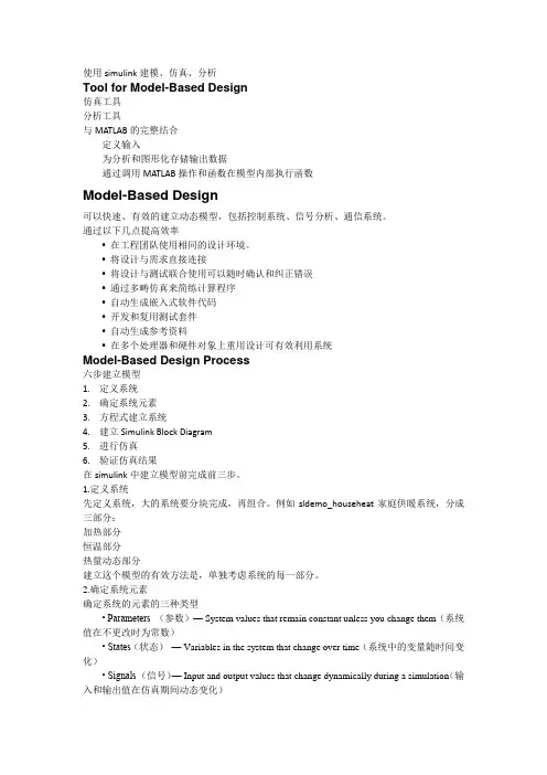
使用simulink建模、仿真、分析Tool for Model-Based Design仿真工具分析工具与MATLAB的完整结合定义输入为分析和图形化存储输出数据通过调用MATLAB操作和函数在模型内部执行函数Model-Based Design可以快速、有效的建立动态模型,包括控制系统、信号分析、通信系统。
通过以下几点提高效率• 在工程团队使用相同的设计环境。
• 将设计与需求直接连接• 将设计与测试联合使用可以随时确认和纠正错误• 通过多畴仿真来简练计算程序• 自动生成嵌入式软件代码•开发和复用测试套件• 自动生成参考资料• 在多个处理器和硬件对象上重用设计可有效利用系统Model-Based Design Process六步建立模型1.定义系统2.确定系统元素3.方程式建立系统4.建立Simulink Block Diagram5.进行仿真6.验证仿真结果在simulink中建立模型前完成前三步。
1.定义系统先定义系统,大的系统要分块完成,再组合。
例如sldemo_househeat家庭供暖系统,分成三部分:加热部分恒温部分热量动态部分建立这个模型的有效方法是,单独考虑系统的每一部分。
2.确定系统元素确定系统的元素的三种类型• Parameters (参数)— System values that remain constant unless you change them(系统值在不更改时为常数)• States(状态)— Variables in the system that change over time(系统中的变量随时间变化)• Signals (信号)— Input and output values that change dynamically during a simulation(输入和输出值在仿真期间动态变化)方程式建立模型第三步,用数学方程式描述系统。
对于每一部分,使用确定的系统元素用数学方式描述系统。


Simulink使用入门下面简要的介绍一下,如何使用Simulink进行建模和仿真实验:1.启动matlab之后,在命令窗口中输入命令“Simulink”或者单击工具栏上的Simulink图标,打开Simulink模块库窗口。
如图1所示。
图1 Simulink模块库窗口2.在Simulink模块库窗口中单击菜单项“File/New/Model”,就可以新建一个Simulink模型文件。
如图2所示。
图2 Simulink 模型文件3.在2中所建立的Simulink文件窗口中单击“File/Save as”,可以修改文件名,并把文件保存在自己所要保存的路径下。
4.双击Communications Blockset,该模块库包含了通信系统中常用的功能模块:Channels(传输信道),Comm Sources(信源),Comm Sink(信宿),Source Cording(信源编码),Modulation(调制),等等。
如图3所示。
图3 通信工具箱里的功能模块5.在Simulink基础库中找到自己需要的模块,选取该模块,直接拖动到新建模型窗口中的适当位置,或者选取该模块后,右击鼠标,“Add to…”加到所建模块窗口中。
图4中,把信号发生器放到了amn中。
图4 利用模块库建立仿真模型6.如果需要对模型模块进行参数设置和修改,只需选中模型文件中的相应模块,单击鼠标右键,选取相应的参数进行修改,或者双击鼠标左键,进行修改。
还可以在选中模块之后通过拖动鼠标来修改模块的位置、大小和形状。
7.通过快捷菜单的其它选项还可以对模型的颜色、旋转、字体、阴影等属性进行设置,也可以对模型进行接剪切、拷贝或删除。
8.模块外部的大于符号“>”分别表示信号的输入输出节点,为了连接两个模型的输入输出,可以将鼠标置于节点处,这时鼠标显示为十字,拖动鼠标到另一个模块的端口,然后释放鼠标的按钮,则形成了带箭头的连线,箭头的方向表示信号的流向。
Simulink操作入门
1、启动MATLAB,在命令窗口输入simulink或单击Simulink工具按钮(如下)。
2、打开的simulink窗口如下。
3、新建模型,使用菜单file/new/model。
4、打开的model窗口如下。
5、将之并列如下(方便操作)。
6、在左侧找到simulink/Soures中的Sine Wave工具,拖至右侧合适位置。
7、同上,分别找到Sinks中的Scope、Signal Routing中的Mux和Continuous中的Integrator 放置如下
8、注意,每个模块图形的左右分别是输入和输出连接点。
9、连接方法,从出发点按住鼠标拖至接收点即可。
结果如下:
10、分支的呢?现将光标点在分支点上,
11、然后按住Ctrl键,拖动鼠标光标到接收点即可。
结果如下:
12、保存模型,File/save,输入文件名即可。
试验运行,单击如下运行按钮。
13、双击Scope,可见图形窗口。
14、命令窗口显示如下。
15、显示是使用了默认值。
通过model窗口的Simulation /Configuration Parameters菜单,可以详细设置各种参数。
参考文献:Matlab/ Simulink/ Help。
simulink指导书Simulink指导书Simulink是一款功能强大的图形化建模和仿真环境。
它是MATLAB 的一个重要扩展模块,用于设计、建模和仿真各种复杂的动态系统。
本篇文章将为您介绍Simulink的基本概念和使用方法,帮助您快速上手并充分发挥其优势。
一、Simulink的基本概念1. 模型:在Simulink中,系统被表示为一个模型。
模型由各种模块组成,每个模块代表系统的一个组成部分,如传感器、执行器、控制器等。
通过将这些模块以图形化的方式连接在一起,我们可以构建出一个完整的系统模型。
2. 模块:Simulink提供了丰富的模块库,包括数学运算、信号处理、控制系统等各类模块。
我们只需从库中拖拽相应的模块到模型中,并通过连接线将其连接起来即可。
3. 信号流:在Simulink中,信号是系统中各个模块之间的信息传递方式。
通过连接线将输入信号传递给模块,模块对信号进行处理后再输出到下一个模块,从而完成整个系统的功能。
4. 仿真:Simulink提供了强大的仿真功能,可以模拟系统在不同条件下的行为。
通过设置各个模块的参数,我们可以观察系统的响应、性能等,并进行优化设计。
二、Simulink的使用方法1. 创建模型:在Simulink界面中,点击“新建模型”按钮,即可创建一个新的模型。
在模型中,我们可以添加各种模块并进行连接。
2. 添加模块:在Simulink界面左侧的模块库中,可以找到各种类型的模块。
可以通过拖拽模块到模型中的方式添加模块。
在添加模块时,可以根据系统的需求选择合适的模块,并设置其参数。
3. 连接模块:在模型中,可以通过连接线将各个模块连接起来,形成信号的传递路径。
连接线可以直接从一个模块的输出端口拖拽到另一个模块的输入端口上。
4. 参数设置:对于每个模块,可以通过双击打开其参数设置对话框,进一步调整其行为。
参数设置可以包括模块的初始状态、输入输出范围、采样时间等。
5. 仿真运行:在模型建立完成后,可以点击Simulink界面上的“运行”按钮,进行仿真运行。
simulink⼊门教程S i m u l i n k⼊门教程-CAL-FENGHAI.-(YICAI)-Company One1Simulink?快速⼊门启动Simulink软件要构建模型,可以使⽤ SimulinkEditor 和 Library Browser。
启动MATLAB软件启动 Simulink 之前,请先启动 MATLAB。
请参阅启动和关闭(MATLAB)。
配置MATLAB以启动Simulink您在 MATLAB 会话中打开第⼀个模型时需要的时间⽐打开后续模型长,因为默认情况下,MATLAB 会在打开第⼀个模型时启动 Simulink。
这种即时启动Simulink 的⽅法可以缩短 MATLAB 启动时间,避免不必要的系统内存占⽤。
要快速打开第⼀个模型,您可以配置 MATLAB,在它启动时同时启动 Simulink。
要启动 Simulink ⽽不打开模型或 Library Browser,请使⽤?start_simulink。
根据 MATLAB 的启动⽅式,恰当使⽤此命令:在 MATLAB?⽂件中在操作系统命令⾏中,使⽤matlab命令和-r开关例如,要在运⾏ MicrosoftWindows操作系统的计算机上启动 MATLAB 时启动Simulink,请创建具有以下⽬标的桌⾯快捷⽅式:matlabroot\bin\win64\ -r start_simulink在 Macintosh 和?Linux计算机上,可在启动 MATLAB 时使⽤以下命令启动Simulink 软件:matlab -r start_simulink打开SimulinkEditor要打开 Simulink Editor,您可以:创建⼀个模型。
在 MATLAB 的?Home选项卡上,点击Simulink并选择⼀个模型模板。
或者,如果您已经打开了 Library Browser,请点击?New Model按钮。
有关创建模型的其他⽅法,请参阅创建模型。
3 Creating a Simulink Model•“Overview of a Simple Model”on page3-2•“Creating the Simple Model”on page3-3•“Connecting Blocks in the Simple Model”on page3-9•“Simulating the Simple Model”on page3-143Creating a Simulink®ModelOverview of a Simple ModelYou can use Simulink software to model dynamic systems and simulate thebehavior of the models.The basic techniques you use to create a simple modelare the same techniques you will use for more complex models.To create this simple model,you need four blocks:•Sine Wave—Generates an input signal for the model.•Integrator—Processes the input signal.•Mux—Multiplexes the input signal and processed signal into a singlesignal.•Scope—Visualizes the signals in the model.After connecting the blocks,they model a system that integrates a sine wavesignal and displays the result along with the original signal.You can build this simple model yourself,starting with“Creating a NewModel”on page3-3.3-2Creating the Simple ModelCreating the Simple ModelIn this section...“Creating a New Model”on page3-3“Adding Blocks to a Model”on page3-4“Moving Blocks in the Model”on page3-8Creating a New ModelBefore creating a model,you need to start Simulink,and then open an emptymodel window.1If Simulink is not running,in the MATLAB Command Window,entersimulinkThe Simulink Library Browser opens.2From the Simulink Library Browser menu,select File>New>Model.A Simulink editor window opens with an empty model in the right pane.3-33Creating a Simulink®Model3Select File>Save as.The Save As dialog box opens.4In the File name box,enter a name for your model,and then click Save.For example,enter simple_model.The software saves your model with the filename simple_model.mdl.Adding Blocks to a ModelTo create a model,you begin by copying blocks from the Simulink LibraryBrowser to the Simulink editor window.For a description of the blocks in thisexample,see“Overview of a Simple Model”on page3-2.1In the Simulink Library Browser,select the Sources library.The Simulink Library Browser displays blocks from the Sources library inthe right pane.3-4Creating the Simple Model3-53Creating a Simulink®Model2Select the Sine Wave block,and then drag it to the editor window.A copy of the Sine Wave block appears in your model.3Add the following blocks to your model in the same way you added theSign Wave block.Library BlockSinks ScopeContinuous IntegratorSignal Routing MuxYour model now has the blocks you need for the simple model.3-6Creating the Simple Model3-73Creating a Simulink®ModelMoving Blocks in the ModelBefore you connect the blocks in your model,you should arrange themlogically to make the signal connections as straightforward as possible.Tomove a block in a model,you can either•Click and drag the block•Select the block,and then press the arrow keys on the keyboard1Move the Scope block after the Mux block output.2Move the Sine Wave and Integrator blocks before the Mux block Inputs.Your model should look similar to the following figure.Your next task is to connect the blocks together with signal lines.See“Connecting Blocks in the Simple Model”on page3-9.3-8Connecting Blocks in the Simple ModelConnecting Blocks in the Simple ModelIn this section...“Block Connections in a Model”on page3-9“Drawing Lines Between Blocks”on page3-9“Drawing a Branch Line”on page3-12Block Connections in a ModelAfter you add blocks to your model,you need to connect them.The connectinglines represent the signals within a model.Most blocks have angle brackets on one or both sides.These angle bracketsrepresent input and output ports:•The>symbol pointing into a block is an input port.•The>symbol pointing out of a block is an output port.Input port Output portDrawing Lines Between BlocksConnect the blocks by drawing lines between output ports and input ports.For how to add blocks to the model in this example,see“Adding Blocks toa Model”on page3-4.1Position your mouse pointer over the output port on the right side of theSine Wave block.3-93Creating a Simulink®Model2Drag a line from the output port to the top input port of the Mux block.While holding the mouse button down,the connecting line is shown as alight colored arrow.3Release the mouse button over the output port.Simulink connects the blocks with an arrow indicating the direction ofsignal flow.4Drag a line from the output port of the Integrator block to the bottom inputport on the Mux block.The Integrator block connects to the Mux block with a signal line.3-10Connecting Blocks in the Simple Model5Select the Mux block,hold down the Shift key,and then select the Scopeblock.A line is drawn between the blocks to connect them.Note The Shift+click shortcut is useful when you are connecting widelyseparated blocks,or when working with complex models.Your model should now look similar to the following figure.3-113Creating a Simulink®ModelDrawing a Branch LineThe simple model is almost complete,but one connection is missing.To finishthe model,you need to connect the Sine Wave block to the Integrator block.This final connection is somewhat different from the other three connections,which all connect output ports to input ports.Because the output port of theSine Wave block already has a connection,you must connect this existing lineto the input port of the Integrator block.The new line,called a branch line,carries the same signal that passes from the Sine Wave block to the Mux block.1Position the mouse pointer on the line between the Sine Wave and theMux block.2Hold down the Ctrl key,and then drag a line to the input port of theIntegrator block input port.This step adds a connection to the existing line and draws a line betweenthe connection and the input port of the Integrator block.3-12Connecting Blocks in the Simple Model3From the File menu,click Save.Your model is now complete.It should look similar to the following figure.After your model is complete,you can simulate the model.See“Simulatingthe Simple Model”on page3-14.3-133Creating a Simulink®ModelSimulating the Simple ModelIn this section...“Setting Simulation Options”on page3-14“Running a Simulation and Observing Results”on page3-15Setting Simulation OptionsBefore you simulate a model,you have to set simulation options.You specifyoptions,such as the stop time and solver,using the Model ConfigurationParameters dialog box.For how to build the model in this example,see“Creating the Simple Model”on page3-3.1In the Simulink editor window,select Simulation>ModelConfiguration Parameters.The Configuration Parameters dialog boxopens to the Solver pane.2In the Stop time field,enter20,and in the Max step size field,enter0.2.3Click OK.The software updates the parameter values with your changes and closesthe Configuration Parameters dialog box.For more information about Simulink configuration parameters,see“Configuration Parameters Dialog Box”.3-14Simulating the Simple Model Running a Simulation and Observing ResultsAfter entering your configuration parameter changes,you are ready tosimulate the simple model and visualize the simulation results.1In the Simulink editor window and from the menu,selectSimulation>Start.The simulation runs,and then stops when it reaches the stop time specifiedin the Model Configuration Parameters dialog box.Tip Alternatively,you can control a simulation by clicking the Startsimulation button and Stop simulation button on the editorwindow toolbar.2Double-click the Scope block.The Scope window opens and displays the simulation results.The plotshows a sine wave signal with the resulting cosine wave signal from theIntegrator block.3-153Creating a Simulink®Model3From the toolbar,click the Parameters button,and then the Graphicstab.The Scope Parameters dialog opens with figure editing commands.4Make changes to the appearance of the figure.For example,select whitefor the Figure and Axes background color,and change the signal line colorsto blue and green.Click the Apply button to see your changes.3-16Simulating the Simple Model5Select File>Close.The Simulink editor window closes with changes to your model and the configuration parameters.3-173Creating a Simulink®Model 3-184 Modeling a Dynamic Control System•“Understanding a Demo Model”on page4-2•“Simulating the Demo Model”on page4-11•“Moving Data Between MATLAB and the Demo Model”on page4-194Modeling a Dynamic Control SystemUnderstanding a Demo ModelIn this section...“Overview of the Demo Model”on page4-2“Opening the Demo Model”on page4-3“Anatomy of the Demo Model”on page4-4“Subsystems in the Demo Model”on page4-5“Subsystems and Masks”on page4-9“Creating a Subsystem”on page4-9“Creating a Subsystem Mask”on page4-10Overview of the Demo ModelThis demo model illustrates how you can use Simulink software to modela dynamic control system.The model defines a heating system and thethermodynamics of a house.It included the outdoor environment,the thermalcharacteristics of a house,and the house heating system.Use this model to explore common Simulink modeling tasks,such as•Grouping multiple blocks into a single subsystem block to simplify a blockdiagram.See“Subsystems in the Demo Model”on page4-5•Customizing the appearance of blocks using the masking feature.See“Creating a Subsystem Mask”on page4-10•Simulating a model and observing the results using a Scope block.See“Running the Simulation”on page4-11•Changing the input parameters of the model to investigate how the systemresponds.See“Changing the Thermostat Setting”on page4-12.•Importing data from the MATLAB workspace into a model beforesimulation.See“Importing Data from the MATLAB Workspace”on page4-19.•Exporting simulation data from the model back to the MATLAB workspace.See“Exporting Simulation Data to the MATLAB Workspace”on page4-23. 4-2Understanding a Demo Model Opening the Demo ModelThe demo model for this example is called sldemo_househeat.It models the heating system and thermodynamics of a house.1Start MATLAB,and then In the MATLAB Command Window,enter sldemo_househeatThe Simulink editor opens with the demo model.4Modeling a Dynamic Control SystemAnatomy of the Demo ModelThe demo model defines the dynamics of the outdoor environment,thethermal characteristics of the house,and the house heating system.It allowsyou to simulate how the thermostat setting and outdoor environment affectthe indoor temperature and cumulative heating costs.The demo model includes many of the same blocks you used to create thesimple model in Chapter3,“Creating a Simulink Model”.These include:•A Scope block(labeled PlotResults)on the far right,displays thesimulation results.•A Mux block at the bottom right,combines the indoor and outdoortemperature signals for the Scope.•A Sine Wave block(labeled Daily Temp Variation)at the bottom left,provides one of three data sources for the model.In the demo model,the thermostat is set to70degrees Fahrenheit.Thesystem models fluctuations in outdoor temperature by applying a sine wavewith amplitude of15degrees to a base temperature of50degrees.The three data inputs(sources)are provided by two Constant blocks(labeledSet Point and Avg Outdoor Temp),and the Sine Wave block(labeled DailyTemp Variation).The Scope block labeled PlotResults is the one output(sink).Understanding a Demo Model Subsystems in the Demo ModelThe sldemo_househeat demo model uses subsystems to simplify theappearance of the block diagram,create reusable components,and customizethe appearance of blocks.A subsystem is a hierarchical grouping of blocks encapsulated by a single Subsystem block.The demo model uses the following subsystems:Thermostat,Heater,House, Fahrenheit to Celsius,and Celsius to Fahrenheit1In the MATLAB Command Window,entersldemo_househeatThe demo model opens in the Simulink editor window.4Modeling a Dynamic Control System2Subsystems can be complex and contain many blocks that might otherwiseclutter a diagram.For example,double-click the House subsystem block toopen it.Contents of House subsystemThe subsystem receives heat flow and external temperature as inputs,which it uses to compute the current room temperature.You could leaveeach of these blocks in the main model window,but combining them as asubsystem helps simplify the block diagram.Understanding a Demo Model3A subsystems can also be simple and contain only a few blocks.Forexample,double-click the Thermostat subsystem block to open it.Contents of Thermostat subsystemThis subsystem models the operation of a thermostat,determining whenthe heating system is on or off.It contains only one Relay block,butlogically represents the thermostat in the block diagram..4Modeling a Dynamic Control SystemUnderstanding a Demo Model Subsystems and MasksSubsystems allows you to group related blocks into one block.They are also reusable,enabling you to implement an algorithm once and use it multiple times.For example,the model contains two instances of identical subsystems named Fahrenheit to Celsius.These subsystems convert the inside and outside temperatures from degrees Fahrenheit to degrees CelsiusYou can customize the appearance of a subsystem by using a process knownas masking.Masking a subsystem allows you to specify a unique icon anddialog box for the Subsystem block.For example,the House and Thermostat subsystems display custom icons that depict physical objects,while the conversion subsystems display custom dialog boxes when you double-clickthem.1Double-click the Fahrenheit to Celsius block.The custom dialog box for the F2C block opens.2To view the underlying blocks in the conversion subsystem,right-click thesubsystem block,point to Mask,and then select Look Under Mask.The editor displays the blocks behind the mask.Creating a SubsystemTo create a subsystem:1In the demo model window,select the set point and Fahrenheit to Celsiusblocks.4Modeling a Dynamic Control System2From the menu,select Diagram>Subsystem&Modeling Reference>Create Subsystem from Selection.The blocks are combined into one subsystem block.For more information about working with subsystems,see“CreatingSubsystems”in the Simulink User’s Guide.Creating a Subsystem MaskTo mask a subsystem:1In the demo model window,right-click the new subsystem block,and thenselect Mask>Add/Edit Mask.The Mask Editor dialog box opens.2From the Command list,select disp(show text in center of block).The dialog box displays the syntax for this command below the list.3In the Icon Drawing commands field,enter disp('SelectTemperature').4Click OK.The software masks the subsystem block with the text you entered.For more information about masking subsystems,see“Working with BlockMasks”in the Simulink User’s Guide.Simulating the Demo ModelSimulating the Demo ModelIn this section...“Running the Simulation”on page4-11“Changing the Thermostat Setting”on page4-12“Changing the Average outdoor Temperature”on page4-14“Changing the Daily Temperature Variation”on page4-16Running the SimulationSimulating the model allows you to observe how the thermostat setting andoutdoor environment affect the indoor temperature and the cumulativeheating cost.1In the demo model window,double-click the Scope block namedPlotResults.The software opens a Scope window that contains two axes with the labelsHeatCost and Temperatures.2From the menu,select Simulation>Start.The software simulates the model.As the simulation runs,the cumulativeheating cost appears on the HeatCost graph at the top of the Scope window.The indoor and outdoor temperatures appear on the Temperatures graphas yellow(top)and magenta(bottom)signals,respectively.4Modeling a Dynamic Control SystemChanging the Thermostat SettingOne of the most powerful benefits of modeling a system with Simulink isthe ability to interactively define the system inputs and observe changes inthe behavior of your model.This allows you to quickly evaluate your modeland validate the simulation results.Change the thermostat setting to68degrees Fahrenheit and observe howthe model responds.1In the Simulink editor window,double-click the Set Point block.TheSource Block Parameters dialog box opens.2In the Constant value field,enter68.Simulating the Demo Model3Click OK.The software applies your changes.4To rerun the simulation,select Simulation>Start.The software simulates the model.In the Scope window,notice that a lower thermostat setting reduces the cumulative heating cost.4Modeling a Dynamic Control SystemChanging the Average outdoor TemperatureChange the average outdoor temperature to45degrees Fahrenheit andobserve how the model responds.1In the Simulink editor window,double-click the Avg Outdoor Temp block.The Source Block Parameters dialog box opens.2In the Constant value field,enter45.Simulating the Demo Model3Click OK.The software applies your changes and closes the dialog box.4To rerun the simulation,select Simulation>Start.The software simulates the model dynamics.In the Scope window,noticethat a colder outdoor temperature increases the cumulative heating cost.4Modeling a Dynamic Control SystemChanging the Daily Temperature VariationDecrease the temperature variation to see how the model responds.1In the Simulink editor window,double-click the Daily Temp Variationblock.The Source Block Parameters dialog box opens.2In the Amplitude field,enter5.3Click OK.The software applies your changes and closes the dialog box.4To rerun the simulation,select Simulation>Start.The software simulates the model.In the Scope window,notice that amore stable outdoor temperature alters the frequency with which theheater operates.Simulating the Demo Model4Modeling a Dynamic Control SystemMoving Data Between MATLAB and the Demo ModelMoving Data Between MATLAB and the Demo ModelIn this section...“Importing Data from the MATLAB Workspace”on page4-19“Exporting Simulation Data to the MATLAB Workspace”on page4-23Importing Data from the MATLAB WorkspaceSimulink also allows you to import data from the MATLAB workspace to themodel input ports.This allows you to import actual physical data into yourmodel.For information about other data import capabilities,see“Importingand Exporting Simulation Data”in the Simulink User’s Guide.Note In this example,you will create a vector of temperature data inMATLAB,and use that data as an input to the Simulink model.To import data from the MATLAB workspace:1In the MATLAB Command Window,create time and temperature data byentering the following commands:x=(0:0.01:4*pi)';y=32+(5*sin(x));z=linspace(0,48,1257)';2In the Simulink editor window,select the Avg Outdoor Temp block,andthen press the Delete key to delete it.3Delete the following items from the model in the same way:•Daily Temp Variation block•Two input signal lines to the Sum block•Sum block4Modeling a Dynamic Control SystemThe model should now look similar to the following figure.Notice that theoutput signal from the Sum block changes to a red,dotted line,indicatingthat it is not connected to a block.4In the demo model window,select View>Library Browser.The Simulink Library Browser window opens.5In the Simulink Library Browser,select the Sources library.6From the Sources library right pane,select the In1block,and then drag itto the model window.Moving Data Between MATLAB and the Demo ModelAn In1block appears in the model window.7Connect the dotted line(originally connected to the Sum block)to the In1 block.8In the Simulink editor window,select Simulation>Configuration Parameters.The Configuration Parameters dialog box opens.9In the menu on the left side of the dialog,select Data Import/Export.The Data Import/Export pane opens.4Modeling a Dynamic Control System10Select the Input check box.11In the Input field,enter[z,y].12Click OK.The software applies your changes and closes the dialog box.13To rerun the simulation,select Simulation>Start.The software simulates the model.In the Scope window,notice that themodel ran using the imported data,showing colder temperatures andhigher heat use.Exporting Simulation Data to the MATLAB Workspace Once you have completed a model,you may want to export your simulation results to MATLAB workspace for further data analysis or visualization.For information about additional data export capabilities,see“Exporting Simulation Data”.To export the HeatCost data from the model to the MATLAB workspace:1In the Simulink Library Browser window,select the Sinks library.2From the Sinks library,select the Out1block,and then drag it to the top right of the demo model window.An Out1block appears in the model window.3Draw a branch line from the HeatCost signal line to the Out1block.For more information,see“Drawing a Branch Line”on page3-12.4Select Simulation>Configuration Parameters.The Configuration Parameters dialog box opens.5From the menu on the left side of the dialog box,select DataImport/Export.The Data Import/Export pane opens.6Select the Time and Output check boxes.7Click OK.The software applies your changes and closes the dialog box.8To rerun the simulation,select Simulation>Start.The software simulates the model and saves the time and HeatCost data to the MATLAB workspace.Notice that the tout and yout variables nowappear in the MATLAB workspace.。