2010 美赛 MCM 优秀论文
- 格式:pdf
- 大小:688.44 KB
- 文档页数:24
Forward and Inverse Treatment Planning Analysis of the ProblemGamma Knife is an advanced treatment unit that supplies stereotactic approach to the treatment of lesions within the head such as tumors and malformations by delivering a single dose of ionizing radiation, which is referred to as a "shot". Every shot emanates from 201 cobalt-60 unit sources in a shielded treatment unit. The 201 beams simultaneously intersect at the same point in space, resulting in a spherical region of high dose. Four kinds of shots with beam widths of 4,8,14,and 18 mm are available for irradiating different size volumes. By combining several shots, relatively larger target volume can be treated with the Gamma Knife. Conventionally, the treatment plan is figured out by experienced neurosurgeons and radiation oncologists, but this empirical plan may be feasible at the price of some damage of critical or normal tissues. So our goal is to automate the treatment planning process for lesions of various sizes and shapes. Namely, given a tumor of some shape and size, we have to determine: the number of shots, the location of each shot, and the diameter of each shot under some constraints to produce a dose distribution that conforms closely to the target volume and confines the dose to the normal tissues to a maximum extent.Assumptions●Gamma Beam is perfectly cylindrical.●Each individual gamma beam is of relatively weak intensity, and thereforehas no affect on any tissues.●Tumor is treated with Gamma Knife in our models.Definitions of Constants and Terms●target volume: tumor;●normal tissues: fine tissues but not dose-sensitive;●critical areas: dose-sensitive tissues.●X i, Y i ,Z i : the coordinates of isocenter;●R i: the diameter of shot iSet Parameters ModelIn this model, we try to produce treatment plans simply under the constraints:no shot protrudes outside the target,no overlapping between any two shots, andcover at least 90% of the target volume by all shots.Based on the discussion in the analysis of the problem, we define the treatment plan as a function of the coordinates of isocenter of each shot and associated diameters:S (x1 , y1 , z1 , R1,……x i , y i , z i , R i,……),where x i , y i , z i is the coordinates of isocenter and R i is the diameter of shot i . To formulate optimal treatment plan under the constraints mentioned above is to decide the parameters included in S . Thus, the whole problem is reduced to a sphere-packing problem, and given a tumor, we employ simulated annealing algorithm to produce the treatment plan S (see Simulated Annealing Algorithm). Although there are several algorithms to deal with the sphere-packing problem, the simulated annealing algorithm is relatively fast, which is appreciated by the users of Gamma Knife. Afterwards, with the fixed parameters in S, we sketch the dose distribution to see whether or not it meets clinical demands. If so, this treatment plan is fit for the present tumor. Clinical Demands●ConstraintsTo protect the normal tissues from lethal dose delivered by all shots, there isone constraint:keep the dose to normal tissue below tolerance doses.For each treatment plan S , we get the different isodose curves. Given a critical tissue, since the tolerance dose is fixed, we use the corresponding isodose curve to evaluate the plan. Assuming the tolerance dose of some tissue is 50%, if the area within the 50% isodose curve includes any part of the tissue, this plan is unsatisfactory. (Both satisfactory-plan and unsatisfactory-plan are shown in Figure 1.)● Optimization DemandsTo guarantee safe and accurate treatment, several optimization demands are as follows:● homogeneity: the doses to points in the target show no significantdifference ,● minimal dose to the entire normal tissues, and●minimal dose delivered to points in critical areas. Since the points of some distance from the isocenter are hardly affected by the shot, we encompass the tumor with a cube, whose size can be determined empirically, and only consider the doses to points within the cube. Assuming that target volume, normal tissues and critical areas are all included in the cube, uniformly we pick N a points, N b points and N c points respectively in the three parts, respectively . We measure the total dose by:∑=Na la la la la z y xU 1),,( in the target volume,),,(∑b b N l lb lb lb z y xU in the normal tissues, and),,(lc lc Nc lc lc z y xU ∑ in the critical areas,where U (x l , y l , z l ) is the total dose delivered to a point by all shots in some treatment plan.∑==Ni i z y x D z y x U 1),,(),,(,where N is the number of shots;∑=⨯⨯⨯⨯=20112),,(),()(),,(m m m m OAR m m TMR m OF m F d R r U d R U R U C z y x DIn the target volume, the maximal dose of one point is),,(max 1la la la N l z y x U a a ≤≤ and the minimal is ),,(min 1la la la N l z y x U a a ≤≤. We measure the dose gradient by the difference:),,(min ),,(max )(11la la la N l la la la N l i z y x U z y x U s U a a a a ≤≤≤≤-=∆The reason why we use ∆U :Since the points is representative of the dose distribution, it is reasonable to believe that the maximum dose of the whole target volume is close to ),,(max 1la la la N l z y x U a a ≤≤, and so is it with the minimum dose. To decrease the dose gradient across the target volume is to make the dose to each point is close as much as possible, so minimizing the difference between the maximum and the minimum dose decrease the gradient to the largest extent.As for points in critical areas every dose of point is strictly constrained so that we have to minimize the maximal dose of all these points. The maximal dose of any point in the critical areas is:),,(max 1lc lc lc N l z y x U ca ≤≤Therefore, for N satisfactory-plans:S i , i =1…Nwe use the following optimization form:⎪⎪⎩⎪⎪⎨⎧-=∆≤≤=≤≤≤≤∑)),,)((max min(),,)((max ),,(min ),,(max )(min 1111c c c c c a a a a l l l i N l Na la la la la i la la la N l la la la N l i z y x S U z y x S U z y x U z y x U s U s.t. }{N i S S S ..1∈where ∆U (S i ) is the ∆U of the i th treatment among the N plansGenerally speaking, no treatment plan S i would satisfy the above three objective functions simultaneously. So we cannot but produce a relative optimal treatment plan from the N plans by assigning three weights α,β,γ to the objective functions. Thus, the single objective function:),,)((max ),,)(()(min 11cc c c c a a a a a l l l i N l N l l l l i i z y x S U z y x S U S U ≤≤=⨯+⨯-∆⨯∑γβαis used to substitute for the multiple objective functions. α,β,γ,differing in importance, are determined with relatively weights on the three objective function, and, obviously, α+β+γ=1.Simulated Annealing AlgorithmTo produce a treatment plan is to determine the parameters of S. Here, we treat the process of setting parameters of plan as a sphere-packing problem. Given a tumor within a brain of certain shape and size, on the surface of the tumor we uniformly pick evenly N sample points from the digital image that consists of millions of points:)z , y , (x i i i 1Ni P ≤≤From the shape and size of the tumor, the number N s of shots that will be delivered, along with the coordinates of isocenter and the diameter of the shot:S (1111,,,R z y x …Ns Ns Ns Ns R z y x ,,,),Where x j , y j , z j are the coordinates of isocenter and R j is the diameter of ith shot in the treatment plan S. We build up a corresponding relationship between sample points P and shots S by the principle that the distance between the point P i and the sphere that represents shot j is the shortest among all the distances from P i to the sphere of other shots. Put simply in mathematics, our objective function in the simulated annealing algorithm is:F (S )= (∑=Ni j i d 12),() / Nj j i j i j i R z z y y x x sqrt j i d --+-+-=])()()[(),(222,where ),(j i d is the distance from point P i to the sphere of its corresponding shot.1. With estimated number of shots, select one possible treatment plan S 0 atrandom, and let the ―temperature‖ T , a parameter in the cooling schedule of the algorithm, high enough.2. Alter S 0 to get another plan S 1 (see How to Get S 1); calculate the objectivefunction with respect to S 0 and S 1, and get the difference: )()(01S F S F F -=∆3. If F ∆<0, then substitute S 1 to S 0; otherwise when the probability Exp{-F ∆/T } is greater than a random value between 0 and 1, the substitution is also necessary.4. Repeat the step 2 and 3 until the process produces a relatively optimaltreatment plan. In practice, we get times L for repetition beforehand.5. Each time reduce the temperature T by ()T λ-1, where λ is a constantthat we assume is 0.9. If the updated temperature T is greater than some certain value, go back to step 2; otherwise terminate the whole process andthus we get the global optimal treatment plan.6. If the percentage of the coverage of the target is less than 90%, we canincrease the number of shots by one and go back to step 1.Besides, with the same process, we introduce another objection function:∑∑==--+-+-=sN j Ni j j i j i j i R z z y y x x sqrt S G 11222)))()()((()(How to Get S 1To get a new treatment plan S 1 based on S 0, we need to alter some or all parameters of S 0. The parameters include the coordinates of isocenter, diameter of each shot. Each time we either increase or decrease coordinates by 0.1mm, whereas change the diameter by 4mm. However, to make sure that any two shots would not overlap, we calculate the distance ),(j i D between any two isocenters. If ),(j i D >R i +R j , the S 1 is obtained.Set the Desired Dose Distribution ModelWhen the constraints are strict, the process of ―trial and err‖ of the ―Set Parameter Model‖ would not work efficiently. For example, when the critical areas are close to the target volume, the process is time consuming. So, in this case, we cannot set the parameters first and measure the treatment plan. Instead, we may as well turn back on the dose distribution to determine the parameters. According to concrete case, we may consider one of the functions below as objective function.Dose to each point :2,,11)(),()(),,(F d s r U d s U s U C z y x D j j j OAK Ns i j TMK Nj OFJ j p t⨯⨯⨯⨯=∑∑==N s is the number of shots , N t =201])sin )(sin cos )(cos cos )(()()()[(2222θβθβϕj j j j j j p y y z z x x z z y y x x sqrt r -+-+---+-+-=θβθβθsin )(cos cos )(cos cos )(j j j p y y z z x x SSD A d -+-+---=Integral dose to tumor: ∑=aN i ii i z y x f 1),,( Maximum dose to tumor: )),,((max 1i i i Ni z y x f ≤≤ Minimum dose to tumor: )),,((min 1i i i Ni z y x f ≤≤ Maximum dose to sensitive tissue or organs: ),,((max 1i i i N i z y x f c≤≤ Maximum dose to critical volumes: ),,((max 1i i i N i z y x f d≤≤ Integral dose to the entire volume of normal tissue or organs:∑=b N i i i i z y x f 1),,(Maximum dose to specified normal tissue points:),,((max 1i i i Ne i z y x f ≤≤⎪⎪⎩⎪⎪⎨⎧-≤≤=≤≤≤≤∑)),,((max min ),,(min ))],,((min ),,((max min[1111i i i N i N i i i i i i i N i i i i N i z y x f z y x f z y x f z y x f d b s.t. :C z y x f i i i Ne i ≤≤≤),,((max 1In fact, this is a multi objective function optimize problem. We give each objective function weights γβα,,, respectively. We also employ simulatedannealing algorithm to find the optimal solution.TestWe write a C++ program to simulate the implementation of our algorithm. For simple manipulation, we suppose that the tumor is egg-shaped in the test, andthe tolerance dose of normal tissues is 50%. We consider two different situations in terms of critical areas, shown in Figure 2. The Figure 2 (a) is the situation where critical areas are almost out of the cube encompassing the tumor, whereas Figure 2 (b) is the situation where critical areas are close tothe target volume.For situation shown in Figure 2 (a), by ―Set Parameters Model‖, we get a setof treatment plans shown in Table 1:TreatmentCoordinates of isocenter and diamaterplan1 (59.58,64.01,50.10,14) (59.73,46.70,61.70,14) (41.24,55.26,58.06,14) (52.93,52.93,40.53,18)2 (48.32,50.32,43.32,14) (58.14,60.07,31.84,14) (56.46,58.44,51.44,14) (58.96,60.96,58.96, 8)3 (53.16,61.78,58.16,14) (39.87,37.87,40.87,18) (65.84,43.83,49.33,14) (38.75,55.75,49.76,18)4 (47.60,49.65,42.50,14) (61.36,63.40,60.20,14) (55.70,57.70,50.70,14) (62.20,44.20,57.50,18)5 (52.32,54.29,47.32,14) (46.82,50.05,50.00,14) (42.70,44.80,39.70, 8) (52.32,54.29,47.32,14)6 (47.56,49.56,42.53,14) (61.46,63.40,37.22,14) (55.74,57.71,50.72,14) (62.20,64.23,57.20, 8)7 (59.40,49.40,61.40,14) (51.20,54.72,50.62,18) (41.62,40.62,61.42,18) (45.95,45.95,33.55,14)Although the all ten-treatment plan is obtained through a process of trail and err, we need to determine which plan is the relatively optimal plan.By the single objective function:),,)((max ),,)(()(min 11c c c c c a a a a a l l l i N l Nl l l l i i z y x S U z y x S U S U ≤≤=⨯+⨯-∆⨯∑γβαs.t.{}10...S Si S i ∈First time, let 4.0,4.0,2.0===γβα, and we get the relatively optimal treatment plan S 10. By calculating the dose of points within the cube, we sketch the isodose curves shown in Figure (3). And in the same way, we get the dose-volume histogram of S 10 shown in Figure (4).Second time, let 5.0,3.0,2.0===γβα, and we get the relatively optimal treatment plan S 4. So situations with different weights generally lead to different optimal plan.As the situation shown in Figure 2( b), the program of ―Set Parameters Model‖ becomes time consumin g, and the treatment generated take little care of the critical areas. So, we suggest that when the critical areas are close to the tumor, it may be much safer and fast to adopt the ―Set the Desired Dose Parameters Model‖Strengths and Weaknesses●StrengthsThe ―Set Parameters Model‖ can give an optimal treatment plan if the tumor is of some distance from the critical areas with high coverage; while the ―Set the Desired Dose Distribution Model‖ guarantees the safety of the critical areas regardless of high coverage.●WeaknessesWe only test our models on the relatively well-defined volume, so thealgorithm can hardly apply to volumes of other shapes.References[1] Y. Sato, N. Shiraga, S. Nakajima, S. Tamura, R. Kikinis, Local maximum intensity projection (LMIP): a new rendering method for vascular visualization, J. Comput. Assisted Tomogr. 22 (6) (1998)912–917.[2] Robert J. Sterootactic Radiosurgery Using the 201 Cobalt—60 Source Gamma knift. Neurosurg Clin North Am,1990,1: 933.[3] D. Vandermeulen, R. Verbreeck, L. Berden, P. Suetents, G. Marchal, Continuous voxel classification by stochastic relaxation: theory and application to MR imaging and MR angiography, Inf. Process. Med. [4] G. Gerig, T. Koller, G. Szekely, C. Brechbuhler, O. Kubler, Symbolic description of 3D structures applied to cerebral vessel tree obtainedfrom MR angiography volume data, Inf. Process. Med. Imaging Lect. Notes Comput. Sci. 687 (1993) 94–111.[5] Shu HZ, Yan YL, Bao XD,et al.Three dimensional optimization oftreatment planning for gamma unit treatment system[J] . Med Phy , 1998,25:2352--2357[6] P.P. Maeder, R.A. Meuli, N. der Tribolet, Three-dimensional volume rendering for magnetic resonance angiography in the screening and preoperative workup of intracranial aneurysms, J. Neurosurg. 85 (6) (1996) 1050–1055.[7] L.O. Hall, A.M. Bensaid, L.P. Clarke, R.P. Velthuizen, M.S. Silboger, J.C. Bezdek, A comparison of neural network and fuzzy clustering techniques in segmenting magnetic resonance images of the brain,IEEE Trans. Neural Network 3 (5) (1992) 672–682.[8] D.G. Health, P.A. Soyer, B.S. Kuszyk, D.F. Bliss, P.S. Calhoun, D.A. Bluemke, M.A. Choti, E.K. Fishman, Three-dimensional spiral CTduring arterial portography: comparison of three rendering technique, Radiographics 15 (4) (1995) 1001–1011.[9] Lunsford LD, Flickinger J, Lindner G, et al . Stereotactic radiosurgery of the brain using the first United States 201 Cobalt-60 source gamma knife . Neurosurgery , 1989,24:151—158 .[10] S. Kobashi, N. Kamiura, Y. Hata, Fuzzy information granulation on segmentation of human brain MR images, J. Jpn Soc. Fuzzy Theory . [11] User’s manual of Leksell gamma unit, Elekta Edition,April 1992 .。

Team#8254page1of16 Play your best hit:The mystery in baseball batMCM Contest Question ATeam#8254February22,2010Contents1Introduction (2)1.1Problem Restatement (2)1.2What is the sweet spot on earth? (2)1.3How to cork a bat? (2)1.4The material of baseball bat matters? (2)2Assumption (3)3A Simplified Model (3)3.1Model Description (3)3.2Finding the”sweet spot” (5)4An Augmented Model (6)4.1Model Description (6)4.2Why no corked bats and metal bats? (8)4.2.1Qualitative Analysis (8)4.2.2Quantitative Analysis (9)5Sensitivity (12)6Conclusion (13)6.1Strength (13)6.2Weakness (13)6.3Recommendation (13)7References (13)8Appendix (14)Team#8254page2of16 1Introduction1.1Problem RestatementEvery experienced hitter knows that there is a spot on the baseball bat that when hitting with this spot,the hand of the hitter feels no pain and the ball can be hit farther.This is the”sweet spot”.According to the theory of torque,this spot should be at the end of the bat,but the experience of the hitters proves it wrong.The location of”sweet spot”on a given baseball bat is approximately 6-1/2”from the end of the bat[1].Our purpose is to establish a model to give a scientific explanation.In addition,some players believe that drilling a cylinder in the end of the bat andfilling it with cork or rubber,namely,to cork the bat [2],enhances the”sweet spot”effect.We would like to found our model and use it to interpret it.What’s more,the question that whether the material of bats matters is also a part discussed in this paper.1.2What is the sweet spot on earth?There are many definitions of”sweet spot”[3].Here in this paper,we define it as the location where maximum energy is transferred to the ball.1.3How to cork a bat?”Corking”is to drill a1inch diameter hole6inches longitudinally into the bat’s barrel end.The structure of the real bat and the corked bat can be showed in Fig1.In our augmented model,we will analyze the effect of corking.1.4The material of baseball bat matters?Compared to the wood bats,aluminum bats is not easily be broke,and as the aluminum bats are hollow,the thickness of the shell can be manipulated so that the center of mass may be more closer to the handle,and consequently reducing the perceived weight while swinging.In this way,it increases the mobility of(a)Normal baseball bat(b)Corked baseball batFig1:Normal baseball bat and corked batTeam#8254page3of16 the hitter.What’s more,using aluminum bat can largely improve the energy of the ejecting ball,which may be too hard to catch or even dangerous for players. All those features lead to the prohibition of the using of aluminum bat[4].We will explain it in details later in this paper.Fig2:Cross section of aluminum bat2AssumptionAs the hitting process is too complex,we make the following assumptions in order to simplify the problems and establish our models:1.The better hitting effect means a larger exit speed of the ball and a shorteracceleration time of the bat.2.When the hitter swings,hitter-bat system rotates around a vertical axis that”penetrates”the hitter.3.The collision of the ball and the bat is one-dimensional.4.The hitter always hits the ball at the”sweet spot”.3A Simplified Model3.1Model DescriptionIn our simplified model,we omit the situations that the player might modify the baseball bat and concentrate on explaining why the”sweet spot”is not at the end of the bat but a few distances from the end.When you hit a ball,the bat vibrates in response.These vibrations travel in waves up and down the length of the bat.At one point,called”the node”, the waves always cancel each other out.If you hit the ball on the bat’s node, the vibrations from the impact will cancel out,and you won’t feel any stinging or shaking in your hand.Since little of the bat’s energy is lost to vibrations when this spot is hit,more can go to the ball[5].We will found a model based onTeam#8254page4of16 the characteristics showed as italics.In our model,we ignore the swing of the hitter’s arms when hit.We denote the spot where the hitter holds the bat as pivot, assuming that the pivot isfixed,and the bat is mounted on the pivot so that it can swing around the pivot freely.The parameters we use are given in the tabular Notation,and the force and motion diagram is showed in Fig3.NotationSymbols MeaningF ball the applied force in the collisionF px,F py the vertical and horizontal component forces of the force in the pivotcm the center of mass of the batp the impact pointpivot the spot where the hitter holds the batI pivot the moment of inertia of the bat with respect to pivotL x−y the distances between x and yαthe rotation angular acceleration of the batm bat the mass of the batL sum the whole length of the batFig3:The force and motion diagram of the batNext,we will analyze the model above with the knowledge of kinetics in order tofind the”sweet spot”.Team #8254page 5of 163.2Finding the ”sweet spot”According to the theorem of moment of momentum we have:F ball ·L pivot =I pivot ·α(1)and based on the theorem of motion of center of mass:∑F =ma c we have:F ball +F px =m bat ·L pivot −cm ·α(2)Therefore,with equation (1)and (2)we have:F hand =F ball m bat ·L pivot −cm ·L pivot −p I pivot−1 Thus we know that the horizontal component force is 0whenL pivot −p =I pivotm bat L pivot −cmIn other words,when the distance between the pivot and the p is I pivot m bat ·L pivot −cm ,the p is the sweet spot.In order to find the specific location of the ”sweet spot”on a certain bat,we quote the data from [6]and choose a C243wooden bat,thus we get the parame-ters L pivot −cm =0.42m ,I pivot =0.208kg ·m 2,L knob −pivot =0.15m ,m bat =0.905kg ,L sum =0.86m .Then we calculate L pivot −p =0.55m ,so that L knob −p =0.70m .From the re-sult we can obviously see that the ”sweet spot”is about 0.16m far from the end of the fat part of the bat.The forces on different location of the bat can be showed in Fig4.Fig 4:The rotation system in a hitting processIn this way,we have successfully demonstrated that the experience of the hitters is right.Team#8254page6of16 4An Augmented Model4.1Model DescriptionThe previous model fails to take the situation that some hitter may modify the bat into account.What’s more,in real baseball game it is impossible that the arms of the hitter are stationary when hit.So we augmented ourfirst model. In this augmented model,we assume that the hitter and the bat form a rotation system in which the hitter stays vertical and the bat stays horizontal.The hitting process can thus be modeled as:the system gets a torque T generated by the hitter and rotates around the axis which vertically”penetrates”the hitter and then hits a ball.After hitting process,the ball ejects out with a velocity of v f. The distance between the impact spot and the axis is r.The process is described in Fig5.Fig5:The rotation system in a hitting processWe notice that the ball gets maximum velocity after hitting means the effect of hitting is optimal,so we should focus on the exit speed of the ball.Two processes are displayed as follows:Process1:The hitter swings the bat and accelerates the bat to an angular velocity ofω.Process2:After the imperfect inelastic collision of bat and ball,the ball ejects out with a velocity of v f.In process1,the moment of inertia of bat and the air resistance will hamper the rotation of the system of hitter-bat.It is easy to calculate the liner velocity of any spot on the bat by the kinematics formula v=ωr,and according to the formulas given by Keith Koenig in reference[7],we know that the angular ve-Team#8254page7of16 locity and the linear velocity of the impact spot on the bat before the collision in process1are:ω=TK Dtanhcosh−1expK DI hitter+I batθv bat=rω(3) where•r is the rotation radius,equals the length from the impact spot to the axis.•T is the torque applied to the hitter-bat system which is generated by the hitter.•K D is an aerodynamic parameter,which is given byK D=12ρC D DL44(for more please read reference[7])•tanh is hyperbolic tangent function.•cosh−1is anti-hyperbolic cosine function.•exp is exponential function.•θis the angle that the bat rotates.•I hitter is the hitter’s moment of inertia with respect to the axis.•I bat is the bat’s moment of inertia with respect to the axis.In our case,we treat T,K D,I hitter,θas constant parameters while r and I bat are the only variables.In process2,we assume that the bat and ball have an one-dimensional col-lision and they both have some extent of deformation.The deformation trans-forms a small part of the kinetic energy(about25%,reference[8])into potential energy stored in bat and ball,while most part(about75%)of it dismisses due to the friction and the oscillation of the bat.And referring to reference[7]we havev f=COR−r M1+r Mv ball+COR+11+r Mv bat(4)where•COR is the coefficient of restitution,it will be discussed in the next part.•v ball is the velocity of the ball right before the collision with the bat.Team #8254page 8of 16•v bat is the velocity of the bat right before the collision with the bat.by equation (3)and (4),we getv f =COR −r M 1+r M v ball +COR +11+r M r T K D tanh cosh −1 exp K D I hitter +I batθ (5)The parameters:COR ,I bat ,r M are explained in Appendix .4.2Why no corked bats and metal bats?In order to reveal the influence of each parameter on the velocity of the ball thus to figure out the effect of the corking behavior and predict different be-havior for wood and metal bats,we make some analysis about the application procedure of our augmented model.4.2.1Qualitative AnalysisWe assume that the velocity of the ball is constant before the collision with the bat,and the impact spots are on the same position of the bat,namely,r is a constant.The corking has two aspects of influences:one is the decrease of mass,the other is the deviation of the center of mass.1.Corked bat•The influence on v fDue to the lower density of material corked in the barrel,the whole mass of bat inclines and the center of mass moves to the rotation axis a little.On one hand,it will cause the decrease of I bat as I bat = r 2dm ,and according to the expression of v f :v f =COR −r M 1+r M v ball +COR +11+r M r T K D tanh cosh −1 exp K D I hitter +I batθ we know that the value of r T K D tanh cosh −1 exp K D I hitter +I batθ will increase.On the other hand,as we haver M =m ball (z −z p )2I cm +m bat L 2pivot −cmTeam#8254page9of16 we know that if m bat decreases and the center of mass deviates toknob,I cm and L pivot−cm will both decline,and that will make r M in-crease and lead to the decline of both COR−r M1+r M v ball and COR+11+r M.How-ever,it is impossible for us to ensure whether the value of v f willincrease or decrease without specific data.We will explain it later inthe Quantitative Analysis section.•The influence onflexibilityWe regard the procedure that the hitter-bat system is accelerated fromstationary situation to rotating with an angular velocity ofωas auniformly accelerated motion procedure.By kinematic formulas weknow that the acceleration time is t=2θω,and from the expression ofωmentioned in page6,section4.1,we know that as the I bat decreasesdue to corking,the value ofωwill increase,so that the accelerationtime will be shorten and in this way theflexibility develops.2.Metal bats vs.wood batsUsing our augmented model we are able to analyze the behavior of bats that have different composition material.•The influence on v fMetal bats(usually aluminum bats)have trampoline effect due togood elasticity,so that it has larger COR than wood bats(usually ashbats).In addition,as the aluminum bats have less mass,the influenceof material is just like that in discussing corked bats.It is obvious thatin order tofind which kind of bat’s v f is larger we need the supportof data.•The influence onflexibilityThe aluminum bats are lighter than wood bats so that the influenceonflexibility is the same as corked bats.4.2.2Quantitative Analysis1.Data usingAs the qualitative analysis cannot show the exact differences between wood bats,corked wood bats(corked bats)and aluminum bats,we quote the data from reference[7][12][13][14]to verify our augmented model.Table1:Value of ConstantsTeam#8254page10of16Constants Valuem ball/(g)134.2v ball/(m/s)25(assumption)T316N·mK D/(N·m·s2)0.00544θ 2.36radr/(m)0.762R hitter−pivot/(m)0.305I hitter/(kg·m2)0.444Table2:Value of VariablesValues Wood bat Corked bat Aluminum batCOR0.500.500.58mass/(g)876834827I p/(kg·m2)0.2110.1950.17L cm−pivot/(cm)424039.5I bat/(kg·m2)0.5160.4760.446z−z p/(m)0.470.460.45r M0.14030.14540.1596 Using the data above we can calculate the three relative values of v f that are47.1m/s,47.6m/s and51.3m/s.The I bat is calculated based on parallel axis theorem.For a better compare of the hitting effects of the three bats,we use com-puter to make a hitting experiment simulation about theflying trajectories of the ball after hitting:Assuming that the ball dose a slanting parabolic motion and the launch angle of the ball after hitting with the bat isθ=30◦.Fig6shows the trajec-tories of balls that are hit by the three kinds of bats.2.The influence of three kinds of bats onflexibilityCombine the formula t=2θωwith the expression ofω,we have the expres-sion of the acceleration time t:t=2θTK Dtanhcosh−1expK DI hitter+I batθAfter using the values given in the table1and table2,we get:Kinds of bats t/(s)Wood Bats0.121Corked Bats0.118Aluminum Bats0.116Team#8254page11of16Fig6:The trajectories of the balls hit by the three kinds of bats It is easy to see that the acceleration time of corked bat is0.003s shorter than that of wood bat.During this time,the incoming ball moves0.075m farther,that is to say,theflying distance of the incoming ball from the ser-vice point to the collision point when using a corked bat is0.075m farther than that of wood bat,so that the hitter would feel more easy to deal with the incoming ball as he or she has more time to react and accelerate the bat when using a corked bat.In the same way we know that when usinga aluminum bat rather than a wood bat,the hitter has0.005s longer and0.125m farther to handle the bat.3.Summary of our analysisAt this point,we are able to answer the second and third questions about the corking behavior and the matters of different materials.•Why does Major League Baseball prohibit”corking”?From the analysis above we know that for a baseball bat used in ourmodel,if it is corked,the swinging velocity of bat right before hittingthe ball will increase0.5m/s and theflexibility of swinging can alsobe developed,as the mass of the bat decreases and the center of massof it deviates.•Why does Major League Baseball prohibit metal bats?According to our model,the hitting effect is closely linked with thematerials.We know from our qualitative verification that the hittingvelocity of using a aluminum bat is4.2m/s more than that of woodbat,and the deviation of the center of mass further gains0.005s reac-tion time for the hitter.As the ball hit by aluminum bat has a muchbigger velocity,it makes the catching of the ball difficult and evendangerous.Team#8254page12of16 5SensitivityAfter analyzing the application of our augmented model,wefind it neces-sary to analyze the sensitivity of our model,aiming at implementing it more effectively.We choose to research the exit speed of normal wood bat with differ-ent parameters.1.The influence of massThe change of mass will influence both r M and I bat,but as the value of them are too hard to obtain by direct calculating,we make some simplificationsbelow:r M=m ball (z−z p)2I p=m ball(z−z p)2I cm+m bat L2pivot−cmIn this expression,as I cm is very small(about0.04kg·m2),we treat it as a constant one.It is the same to z−z p(about0.47m)and L pivot−cm(about 0.42m).Hence,the value of r M only correlates to m bat,and we haver M=0.1340.4720.04+m bat×0.422then in I bat=I cm+m bat·L2hitter−cm,we also treat L hitter−cm(about0.725m) as a constant,so we haveI bat=0.04+m bat×0.7252Relating to equation(5),we denote COR=0.5and get:m bat(kg)0.830.850.870.89v f(m/s)46.846.7646.7146.672.The influence of materialThe major influence of different materials is they have different COR s.When the mass is constant,we have I bat=0.516kg·m2,and r M=0.1403, andfinally we get:COR0.40.450.50.550.6v f/(m/s)42.344.747.149.551.9From the results above,we can see that COR seems a more prominent influence.Team#8254page13of16 6Conclusion6.1StrengthFirst of all,this paper solves the problem of”sweet spot”,and we give an easy formula to calculate the position of”sweet spot”.Secondly,we analyze the hitting process and divide it into two stages,and discuss the factors that affect the exit speed in details while giving a formula that can describe this stage.Then we answer the questions through qualitative analysis and quantitative calculation.Finally,we make a analysis about the sensitivity and prove the rationality by comparing the results.6.2WeaknessFirst of all,as the real hitting process is too complex to analyze,we make several simplifications in order to facilitate the founding of model.In model 1,we just regard the bat as a pendulum rod with one endfixed,which is a little different from the real situation.And in model2,we simplify the complex process of hitting into two stages.Secondly,the data wefind are not precise,especially for the value of COR which we regard as constant.Additionally,the calculations in this paper are also simplified,thus the accu-racy of our results declines.6.3RecommendationThe biggest disadvantage of our model is lacking experiments,and if we have time and facilities to do some experiments,the result must be more reliable.For example,the equation(6)in Appendix can be used to measure COR,and in order to measure the value of I pivot,we could refer to[15]and use the method to obtain data.With this data we can verify our model in a better way.7References[1]/wiki/Sweet spot[2]/drussell/bats-new/corkedbat.html[3]/drussell/bats-new/sweetspot.html[4]/wiki/Aluminum Bats vs.Wood Bats[5]/baseball/sweetspot.htmlTeam#8254page14of16[6]/sysengr/slides/baseballBat.ppt[7]Keith Koenig,Nan Davis Mitchell,Thomas E.Hannigan,J.Keith Clutter.The influence of moment of inertia on baseball/softball bat swing speed.SportsEngineedng(2004)7,105-117.[8]Alan M.Nathana.Characterizing the performance of baseball bats.Am.J.Phys.,Vol.71,No.2,February2003134-143[9]/wiki/Coefficient of restitution[10]Lv ZhongjieHuang Fenglei.Coefficient of Restitution of a Circular PlateDuring Inelastic Collision.Transactions of Beijing Institute of Technology.Vol.28No.4.[11]P.J.Drane and J.A.Sherwood.Characterization of the effect of temperatureon baseball COR performance.[12]/sysengr/slides/baseballBat.ppt[13]/docs/621958/How-Does-a-Baseball-Bat-Work[14]/wiki/moment of inertia[15]/drussell/bats-new/bat-moi.html8AppendixParameters ExplanationIn expression(5),page8,section4.1,there are several parameters that will influence thefinal velocity of the ball:1.COR•What is COR?The coefficient of restitution(COR),or bounciness of an object is afractional value representing the ratio of velocities after and before animpact[9].Fig7:The one-dimensional collision processTeam #8254page 15of 16The coefficient of restitution is given byCOR =v 1f −v 2f v 1−v 2(6)where–v 1is the velocity of object 1before the collision.–v 2is the velocity of object 2before the collision.–v 1f is the velocity of object 1after the collision.–v 2f is the velocity of object 2after the collision.All the parameters above are scalars.In the ideal situations,we may have a so-called plastic collision when COR =0,namely the deformation of the material cannot re-store.And when COR =1,called perfectly elastic collision,is a situa-tion that the deformation can restore entirely.In general,the value of COR varies from (0,1).•What factors affect COR ?MaterialCOR represents the deformation recovery ability of the material.Gen-erally speaking,the more elastic the material is,the higher the value of COR will be.Impact velocityCOR decreases when the impact velocity increases.[10]The Temperature and Relative Humility of The EnvironmentCompared to the factors above,another two factors,the tempera-ture and relative humility have a relatively smaller influence.COR decreases when the temperature decreases and it decreases when the relative humility increases.[11]2.I bat•MOI (moment of inertia)[14]Moment of inertia is a measure of an object’s resistance to changes in its rotation rate.It is the rotational analog of mass,the inertia of a rigid rotating body with respect to its rotation.The moment of iner-tia plays much the same role in rotational dynamics as mass does in linear dynamics,determining the relationship between angular mo-mentum and angular velocity,torque and angular acceleration,and several other quantities.It is denoted asI = r 2dmwhere m is mass and r is the perpendicular distance to the axis of rotation.Team#8254page16of16•Parallel Axis TheoremI z=I cm+mL2where I cm is the moment of inertia of the rotor with respect to thecenter of mass,and the L is the distance from the center of mass toaxis z.•The factors affect MOIFigure:It influences the location of the center of mass,thereby affectsthe distance from the center of mass to rotation axis.Mass:Its increase is proportional to the increase of MOI.3.r MIn reference[8],Alan M.Nathan develops a formula relating v f to the initial speed of the ball v ball and the initial speed of the bat at the impact pointv bat as:r M=m ball (z−z p)2I pwhere•m ball and m bat are the ball and the bat’s mass respectively.•Z is the location of the impact point.•Z p is the location of the pivot point.•I p is the moment of inertia of the bat with respect to the pivot point. From the expression above we can see that reducing the mass of the bat m bat while keeping the other parameters constant will lead to a augment of r m.。

For office use onlyT1________________ T2________________ T3________________ T4________________Team Control Number7018Problem ChosencFor office use onlyF1________________F2________________F3________________F4________________ SummaryThe article is aimed to research the potential impact of the marine garbage debris on marine ecosystem and human beings,and how we can deal with the substantial problems caused by the aggregation of marine wastes.In task one,we give a definition of the potential long-term and short-term impact of marine plastic garbage. Regard the toxin concentration effect caused by marine garbage as long-term impact and to track and monitor it. We etablish the composite indicator model on density of plastic toxin,and the content of toxin absorbed by plastic fragment in the ocean to express the impact of marine garbage on ecosystem. Take Japan sea as example to examine our model.In ask two, we designe an algorithm, using the density value of marine plastic of each year in discrete measure point given by reference,and we plot plastic density of the whole area in varies locations. Based on the changes in marine plastic density in different years, we determine generally that the center of the plastic vortex is East—West140°W—150°W, South—North30°N—40°N. According to our algorithm, we can monitor a sea area reasonably only by regular observation of part of the specified measuring pointIn task three,we classify the plastic into three types,which is surface layer plastic,deep layer plastic and interlayer between the two. Then we analysis the the degradation mechanism of plastic in each layer. Finally,we get the reason why those plastic fragments come to a similar size.In task four, we classify the source of the marine plastic into three types,the land accounting for 80%,fishing gears accounting for 10%,boating accounting for 10%,and estimate the optimization model according to the duel-target principle of emissions reduction and management. Finally, we arrive at a more reasonable optimization strategy.In task five,we first analyze the mechanism of the formation of the Pacific ocean trash vortex, and thus conclude that the marine garbage swirl will also emerge in south Pacific,south Atlantic and the India ocean. According to the Concentration of diffusion theory, we establish the differential prediction model of the future marine garbage density,and predict the density of the garbage in south Atlantic ocean. Then we get the stable density in eight measuring point .In task six, we get the results by the data of the annual national consumption ofpolypropylene plastic packaging and the data fitting method, and predict the environmental benefit generated by the prohibition of polypropylene take-away food packaging in the next decade. By means of this model and our prediction,each nation will reduce releasing 1.31 million tons of plastic garbage in next decade.Finally, we submit a report to expediction leader,summarize our work and make some feasible suggestions to the policy- makers.Task 1:Definition:●Potential short-term effects of the plastic: the hazardeffects will be shown in the short term.●Potential long-term effects of the plastic: thepotential effects, of which hazards are great, willappear after a long time.The short- and long-term effects of the plastic on the ocean environment:In our definition, the short-term and long-term effects of the plastic on the ocean environment are as follows.Short-term effects:1)The plastic is eaten by marine animals or birds.2) Animals are wrapped by plastics, such as fishing nets, which hurt or even kill them.3)Deaden the way of the passing vessels.Long-term effects:1)Enrichment of toxins through the food chain: the waste plastic in the ocean has no natural degradation in theshort-term, which will first be broken down into tinyfragments through the role of light, waves,micro-organisms, while the molecular structure has notchanged. These "plastic sands", easy to be eaten byplankton, fish and other, are Seemingly very similar tomarine life’s food,causing the enrichment and delivery of toxins.2)Accelerate the greenhouse effect: after a long-term accumulation and pollution of plastics, the waterbecame turbid, which will seriously affect the marineplants (such as phytoplankton and algae) inphotosynthesis. A large number of plankton’s deathswould also lower the ability of the ocean to absorbcarbon dioxide, intensifying the greenhouse effect tosome extent.To monitor the impact of plastic rubbish on the marine ecosystem:According to the relevant literature, we know that plastic resin pellets accumulate toxic chemicals , such as PCBs、DDE , and nonylphenols , and may serve as a transport medium and soure of toxins to marine organisms that ingest them[]2. As it is difficult for the plastic garbage in the ocean to complete degradation in the short term, the plastic resin pellets in the water will increase over time and thus absorb more toxins, resulting in the enrichment of toxins and causing serious impact on the marine ecosystem.Therefore, we track the monitoring of the concentration of PCBs, DDE, and nonylphenols containing in the plastic resin pellets in the sea water, as an indicator to compare the extent of pollution in different regions of the sea, thus reflecting the impact of plastic rubbish on ecosystem.To establish pollution index evaluation model: For purposes of comparison, we unify the concentration indexes of PCBs, DDE, and nonylphenols in a comprehensive index.Preparations:1)Data Standardization2)Determination of the index weightBecause Japan has done researches on the contents of PCBs,DDE, and nonylphenols in the plastic resin pellets, we illustrate the survey conducted in Japanese waters by the University of Tokyo between 1997 and 1998.To standardize the concentration indexes of PCBs, DDE,and nonylphenols. We assume Kasai Sesside Park, KeihinCanal, Kugenuma Beach, Shioda Beach in the survey arethe first, second, third, fourth region; PCBs, DDE, andnonylphenols are the first, second, third indicators.Then to establish the standardized model:j j jij ij V V V V V min max min --= (1,2,3,4;1,2,3i j ==)wherej V max is the maximum of the measurement of j indicator in the four regions.j V min is the minimum of the measurement of j indicatorstandardized value of j indicator in i region.According to the literature [2], Japanese observationaldata is shown in Table 1.Table 1. PCBs, DDE, and, nonylphenols Contents in Marine PolypropyleneTable 1 Using the established standardized model to standardize, we have Table 2.In Table 2,the three indicators of Shioda Beach area are all 0, because the contents of PCBs, DDE, and nonylphenols in Polypropylene Plastic Resin Pellets in this area are the least, while 0 only relatively represents the smallest. Similarly, 1 indicates that in some area the value of a indicator is the largest.To determine the index weight of PCBs, DDE, and nonylphenolsWe use Analytic Hierarchy Process (AHP) to determine the weight of the three indicators in the general pollution indicator. AHP is an effective method which transforms semi-qualitative and semi-quantitative problems into quantitative calculation. It uses ideas of analysis and synthesis in decision-making, ideally suited for multi-index comprehensive evaluation.Hierarchy are shown in figure 1.Fig.1 Hierarchy of index factorsThen we determine the weight of each concentrationindicator in the generall pollution indicator, and the process are described as follows:To analyze the role of each concentration indicator, we haveestablished a matrix P to study the relative proportion.⎥⎥⎥⎦⎤⎢⎢⎢⎣⎡=111323123211312P P P P P P P Where mn P represents the relative importance of theconcentration indicators m B and n B . Usually we use 1,2,…,9 and their reciprocals to represent different importance. The greater the number is, the more important it is. Similarly, the relative importance of m B and n B is mn P /1(3,2,1,=n m ).Suppose the maximum eigenvalue of P is m ax λ, then theconsistency index is1max --=n nCI λThe average consistency index is RI , then the consistencyratio isRICI CR = For the matrix P of 3≥n , if 1.0<CR the consistency isthougt to be better, of which eigenvector can be used as the weight vector.We get the comparison matrix accoding to the harmful levelsof PCBs, DDE, and nonylphenols and the requirments ofEPA on the maximum concentration of the three toxins inseawater as follows:⎥⎥⎥⎦⎤⎢⎢⎢⎣⎡=165416131431P We get the maximum eigenvalue of P by MATLAB calculation0012.3max =λand the corresponding eigenvector of it is()2393.02975.09243.0,,=W1.0042.012.1047.0<===RI CI CR Therefore,we determine the degree of inconsistency formatrix P within the permissible range. With the eigenvectors of p as weights vector, we get thefinal weight vector by normalization ()1638.02036.06326.0',,=W . Defining the overall target of pollution for the No i oceanis i Q , among other things the standardized value of threeindicators for the No i ocean is ()321,,i i i i V V V V = and the weightvector is 'W ,Then we form the model for the overall target of marine pollution assessment, (3,2,1=i )By the model above, we obtained the Value of the totalpollution index for four regions in Japanese ocean in Table 3T B W Q '=In Table3, the value of the total pollution index is the hightest that means the concentration of toxins in Polypropylene Plastic Resin Pellets is the hightest, whereas the value of the total pollution index in Shioda Beach is the lowest(we point up 0 is only a relative value that’s not in the name of free of plastics pollution)Getting through the assessment method above, we can monitor the concentration of PCBs, DDE and nonylphenols in the plastic debris for the sake of reflecting the influence to ocean ecosystem.The highter the the concentration of toxins,the bigger influence of the marine organism which lead to the inrichment of food chain is more and more dramatic.Above all, the variation of toxins’ concentration simultaneously reflects the distribution and time-varying of marine litter. We can predict the future development of marine litter by regularly monitoring the content of these substances, to provide data for the sea expedition of the detection of marine litter and reference for government departments to make the policies for ocean governance.Task 2:In the North Pacific, the clockwise flow formed a never-ending maelstrom which rotates the plastic garbage. Over the years, the subtropical eddy current in North Pacific gathered together the garbage from the coast or the fleet, entrapped them in the whirlpool, and brought them to the center under the action of the centripetal force, forming an area of 3.43 million square kilometers (more than one-third of Europe) .As time goes by, the garbage in the whirlpool has the trend of increasing year by year in terms of breadth, density, and distribution. In order to clearly describe the variability of the increases over time and space, according to “Count Densities of Plastic Debris from Ocean Surface Samples North Pacific Gyre 1999—2008”, we analyze the data, exclude them with a great dispersion, and retain them with concentrated distribution, while the longitude values of the garbage locations in sampled regions of years serve as the x-coordinate value of a three-dimensional coordinates, latitude values as the y-coordinate value, the Plastic Count per cubic Meter of water of the position as the z-coordinate value. Further, we establish an irregular grid in the yx plane according to obtained data, and draw a grid line through all the data points. Using the inverse distance squared method with a factor, which can not only estimate the Plastic Count per cubic Meter of water of any position, but also calculate the trends of the Plastic Counts per cubic Meter of water between two original data points, we can obtain the unknown grid points approximately. When the data of all the irregular grid points are known (or approximately known, or obtained from the original data), we can draw the three-dimensional image with the Matlab software, which can fully reflect the variability of the increases in the garbage density over time and space.Preparations:First, to determine the coordinates of each year’s sampled garbage.The distribution range of garbage is about the East - West 120W-170W, South - North 18N-41N shown in the “Count Densities of Plastic Debris from Ocean Surface Samples North Pacific Gyre 1999--2008”, we divide a square in the picture into 100 grids in Figure (1) as follows:According to the position of the grid where the measuring point’s center is, we can identify the latitude and longitude for each point, which respectively serve as the x- and y- coordinate value of the three-dimensional coordinates.To determine the Plastic Count per cubic Meter of water. As the “Plastic Count per cubic Meter of water” provided by “Count Densities of P lastic Debris from Ocean Surface Samples North Pacific Gyre 1999--2008”are 5 density interval, to identify the exact values of the garbage density of one year’s different measuring points, we assume that the density is a random variable which obeys uniform distribution in each interval.Uniform distribution can be described as below:()⎪⎩⎪⎨⎧-=01a b x f ()others b a x ,∈We use the uniform function in Matlab to generatecontinuous uniformly distributed random numbers in each interval, which approximately serve as the exact values of the garbage density andz-coordinate values of the three-dimensional coordinates of the year’s measuring points.Assumptions(1)The data we get is accurate and reasonable.(2)Plastic Count per cubic Meter of waterIn the oceanarea isa continuous change.(3)Density of the plastic in the gyre is a variable by region.Density of the plastic in the gyre and its surrounding area is interdependent , However, this dependence decreases with increasing distance . For our discussion issue, Each data point influences the point of each unknown around and the point of each unknown around is influenced by a given data point. The nearer a given data point from the unknown point, the larger the role.Establishing the modelFor the method described by the previous,we serve the distributions of garbage density in the “Count Pensities of Plastic Debris from Ocean Surface Samples North Pacific Gyre 1999--2008”as coordinates ()z y,, As Table 1:x,Through analysis and comparison, We excluded a number of data which has very large dispersion and retained the data that is under the more concentrated the distribution which, can be seen on Table 2.In this way, this is conducive for us to get more accurate density distribution map.Then we have a segmentation that is according to the arrangement of the composition of X direction and Y direction from small to large by using x co-ordinate value and y co-ordinate value of known data points n, in order to form a non-equidistant Segmentation which has n nodes. For the Segmentation we get above,we only know the density of the plastic known n nodes, therefore, we must find other density of the plastic garbage of n nodes.We only do the sampling survey of garbage density of the north pacificvortex,so only understand logically each known data point has a certain extent effect on the unknown node and the close-known points of density of the plastic garbage has high-impact than distant known point.In this respect,we use the weighted average format, that means using the adverse which with distance squared to express more important effects in close known points. There're two known points Q1 and Q2 in a line ,that is to say we have already known the plastic litter density in Q1 and Q2, then speculate the plastic litter density's affects between Q1、Q2 and the point G which in the connection of Q1 and Q2. It can be shown by a weighted average algorithm22212221111121GQ GQ GQ Z GQ Z Z Q Q G +*+*=in this formula GQ expresses the distance between the pointG and Q.We know that only use a weighted average close to the unknown point can not reflect the trend of the known points, we assume that any two given point of plastic garbage between the changes in the density of plastic impact the plastic garbage density of the unknown point and reflecting the density of plastic garbage changes in linear trend. So in the weighted average formula what is in order to presume an unknown point of plastic garbage density, we introduce the trend items. And because the greater impact at close range point, and thus the density of plastic wastes trends close points stronger. For the one-dimensional case, the calculation formula G Z in the previous example modify in the following format:2212122212212122211111112121Q Q GQ GQ GQ Q Q GQ Z GQ Z GQ Z Z Q Q Q Q G ++++*+*+*=Among them, 21Q Q known as the separation distance of the known point, 21Q Q Z is the density of plastic garbage which is the plastic waste density of 1Q and 2Q for the linear trend of point G . For the two-dimensional area, point G is not on the line 21Q Q , so we make a vertical from the point G and cross the line connect the point 1Q and 2Q , and get point P , the impact of point P to 1Q and 2Q just like one-dimensional, and the one-dimensional closer of G to P , the distant of G to P become farther, the smaller of the impact, so the weighting factor should also reflect the GP in inversely proportional to a certain way, then we adopt following format:221212222122121222211111112121Q Q GQ GP GQ GQ Q Q GQ GP Z GQ Z GQ Z Z P Q Q Q Q G ++++++*+*+*=Taken together, we speculated following roles:(1) Each known point data are influence the density of plastic garbage of each unknown point in the inversely proportional to the square of the distance;(2) the change of density of plastic garbage between any two known points data, for each unknown point are affected, and the influence to each particular point of their plastic garbage diffuse the straight line along the two known particular point; (3) the change of the density of plastic garbage between any two known data points impact a specific unknown points of the density of plastic litter depends on the three distances: a. the vertical distance to a straight line which is a specific point link to a known point;b. the distance between the latest known point to a specific unknown point;c. the separation distance between two known data points.If we mark 1Q ,2Q ,…,N Q as the location of known data points,G as an unknown node, ijG P is the intersection of the connection of i Q ,j Q and the vertical line from G to i Q ,j Q()G Q Q Z j i ,,is the density trend of i Q ,j Q in the of plasticgarbage points and prescribe ()G Q Q Z j i ,,is the testing point i Q ’ s density of plastic garbage ,so there are calculation formula:()()∑∑∑∑==-==++++*=Ni N ij ji i ijGji i ijG N i Nj j i G Q Q GQ GPQ Q GQ GP G Q Q Z Z 11222222111,,Here we plug each year’s observational data in schedule 1 into our model, and draw the three-dimensional images of the spatial distribution of the marine garbage ’s density with Matlab in Figure (2) as follows:199920002002200520062007-2008(1)It’s observed and analyzed that, from 1999 to 2008, the density of plastic garbage is increasing year by year and significantly in the region of East – West 140W-150W, south - north 30N-40N. Therefore, we can make sure that this region is probably the center of the marine litter whirlpool. Gathering process should be such that the dispersed garbage floating in the ocean move with the ocean currents and gradually close to the whirlpool region. At the beginning, the area close to the vortex will have obviously increasable about plastic litter density, because of this centripetal they keeping move to the center of the vortex ,then with the time accumulates ,the garbage density in the center of the vortex become much bigger and bigger , at last it becomes the Pacific rubbish island we have seen today.It can be seen that through our algorithm, as long as the reference to be able to detect the density in an area which has a number of discrete measuring points,Through tracking these density changes ,we Will be able to value out all the waters of the density measurement through our models to determine,This will reduce the workload of the marine expedition team monitoring marine pollution significantly, and also saving costs .Task 3:The degradation mechanism of marine plasticsWe know that light, mechanical force, heat, oxygen, water, microbes, chemicals, etc. can result in the degradation of plastics . In mechanism ,Factors result in the degradation can be summarized as optical ,biological,and chemical。

承诺书我们仔细阅读了中国大学生数学建模竞赛的竞赛规则。
我们完全明白,在竞赛开始后参赛队员不能以任何方式(包括电话、电子邮件、网上咨询等)与队外的任何人(包括指导教师)研究、讨论与赛题有关的问题。
我们知道,抄袭别人的成果是违反竞赛规则的,如果引用别人的成果或其他公开的资料(包括网上查到的资料),必须按照规定的参考文献的表述方式在正文引用处和参考文献中明确列出。
我们郑重承诺,严格遵守竞赛规则,以保证竞赛的公正、公平性。
如有违反竞赛规则的行为,我们将受到严肃处理。
我们参赛选择的题号是(从A/B/C/D中选择一项填写): C我们的参赛报名号为(如果赛区设置报名号的话):1328303所属学校(请填写完整的全名):武汉职业技术学院参赛队员(打印并签名):1. XXX2. XXX3. X X指导教师或指导教师组负责人(打印并签名):数模指导组日期:2010年9月12日赛区评阅编号(由赛区组委会评阅前进行编号):编号专用页赛区评阅编号(由赛区组委会评阅前进行编号):全国统一编号(由赛区组委会送交全国前编号):全国评阅编号(由全国组委会评阅前进行编号):输油管的布置摘要本文对输油管线的布置主要从建设费用最省的角度进行研究。
首先,对问题一,我们按照共用管线与非共用管线铺设费用相同或不相同,进行分类讨论。
为了更好的说明,我们根据共用管线与非共用管线铺设费用相同或不同及两炼油厂连线与铁路线垂直或不垂直分成四类讨论。
其次,对问题二,由于需要考虑在城区中铺设管线,涉及到拆迁补偿费等。
通过对三个公司的估算费用加权,求得期望值021.5P (万元)。
并利用建立的规划模型②求得管道建设的最省费用为282.70万元。
其中共用管线长度为1.85千米,炼油厂B在城区铺设的管道线对城郊分界线的射影为0.63千米。
最后,对问题三,由于炼油厂A和B的输油管线铺设费用不同,所以最短管道长度和未必能保证铺设总费用最省,因而我们又建立了规划模型③,通过LINGO软件求得管道建设的最省费用为251.97万元,三种管道的结合点O到炼油厂A与铁路垂线的距离为6.13千米,结合点O到铁路的距离为0.14千米,炼油厂B在城区铺设的管道线对城郊分界线的射影为0.72千米。

INERTIAL AND VIBRATIONAL CHARACTERISTICS OF SOFTBALL AND BASEBALL BATS: RESEARCH AND DESIGN IMPLICATIONSLarry Noble, Kansas State University, Manhattan, USA INTRODUCTION: The design of baseball and softball bats has been an ongoing process since the inception of the game in the early 19th century. Until the early 1970's, the only material to be used was wood and the potential for design improvements was limited because they involved changing the physical dimensions of the bat. Also, most of the changes were initiated by the player and were carried out by local craftsmen in wood shops. However, with the introduction of hollow-wall aluminum bats in the 1970's and other metal alloys as well as composite materials since then, the potential for applying relevant mechanical principles to improve the performance characteristics of bats has improved dramatically. In recent years a plethora of bats with innovative features have become available to the consumer. Some of these innovations are a result of the research and development efforts of the bat manufacturing industry, often in collaboration with scientists not directly affiliated with the industry, while others are a result of flawed ideas that are not completely thought through. Braham (1997) provides a recent, up-to-date summary of recent innovations by the leading bat manufacturers, but an evaluation of the claims of these products using relevant criteria is lacking. The purpose of this paper is to provide a scientific basis and a focus for examining and developing new bat design features. The paper will provide an overview of the factors that are relevant to the design of baseball and softball bats, including related theoretical and empirical studies.Factors relevant to the design of baseball and softball batsWhen developing or evaluating a design feature of a baseball or softball bat, the following factors must be considered: (1) the manner in which the bat is swung and forces are transmitted to the bat during the swing, (2) the constraints resulting from rules in the particular sport, and (3) the relevant properties of the bat. I will review each of these general factors in detail, making reference to related scientific literature.Characteristics of batting relevant to bat designBaseball and softball batting is a two-handed sidearm striking skill with the bat held near one end and swung as a physical pendulum. Power hitters attempt to impart maximum velocity to the impacted ball in the desired direction by generating maximum linear velocity of the impacting part of the bat to the ball. The motion of the bat is predominantly in the horizontal plane and the rotation axis ranges from .15 to.20 m off the knob end of the bat toward the hitter’s body during the swing. During the swing, the maximum linear (COP) and rotational velocity of the bat is approximately 33 m/s and 36 r/s, respectively, for college females and 38 m/s and 44 r/s, respectively, for college males. Because the primary goal of the power swing is to maximize bat velocity on impact, it is somewhat surprising that maximum bat velocity has repeatedly been found at from .01 to .05 s prior to impact (Shapiro, 1974; McIntyre & Pfautsch, 1982; Messier & Owen, 1984; Spragg, 86 ISBS'98 –Proceedings II1986). While this finding has been reported in the scientific literature frequently, a plausible explanation of the reason has not been found. A review of the elastic properties of the bat (appearing later in this paper) and the characteristics of the swing may provide a tenable hypothesis. It is possible that, at the beginning of the swing, torque applied to the bat handle to rotate the bat toward the incoming ball and the inertia of the barrel end of the bat cause the bat to bend, with the barrel of the bat lagging behind. This bending mode, usually referred to as the diving board mode , would begin to release when the rotational acceleration of the bat begins to drop. It is conjectured that the elite hitter learns through trial and error to adopt a bat and swing that are matched such that the velocity of the impact point of the bat is maximized at impact. To accomplish this end, accelerating forces would be reduced quickly at either 1/4 or 1 3/4 of the period of oscillation of the diving board mode. For example, if the fundamental, diving board mode of a bat is 25 Hz, then the period of oscillation is 40 ms. For the hitter to take advantage of this elastic behavior, this bending mode would need to be …released“ at approximately 10 or 70 ms prior to impact. While this characteristic of the skilled golf swing has been empirically verified (Cochran & Stobbs, 1986), no empirical data in support of this hypothesis applied to softball or baseball bats have been found.Rules most relevant to bat designThe rules regarding baseball bat characteristics are different from those regarding softball bats. Also, rules are different for different genders and different levels of play. For adult males, the maximum baseball and softball bat barrel size is 2.25 and 2.75 in (.057 and .070 m), respectively. The maximum bat length is 42 and 34 inches (1.067 and .864 m) for baseball and softball, respectively, while the maximum softball bat weight is 38 oz (10.569 N). There is no maximum baseball bat weight. All bats used in professional baseball must be made of wood. The most recent rule, which places an upper limit on the coefficient of restitution (Bat Performance Factor) for bats at different levels and types of play, is having a tremendous impact on the direction of bat design activity. Bat performance factor will be discussed in greater detail later in this paper.Inertial and vibrational properties relevant to bat designSeveral inertial and vibrational properties of the bat are relevant to its effective use: (1) mass, (2) moment of inertia, (3) coefficient of restitution, (4) location of node of the fundamental vibration node, and (5) center of percussion location.Mass and moment of inertia determine the amount of effort required to swing the bat. There is an inverse relationship between bat linear and angular acceleration and mass and moment of inertia, respectively, for a given linear and angular impulse (integral of force/torque and time). Thus, the more mass and/or moment of inertia, the more impulse required to produce a given change in bat speed or direction. In other words, greater mass and moment of inertia compromise the hitter’s ability to control the path of the bat as it moves toward the ball as well as to generate bat velocity during the swing. Theoretical models of the relationship between mass and impact parameters indicate that lighter bats than have been used by most skilled players would be more effective (Kirkpatrick, 1963; Adair, 1990). In a study which sought to empirically determine an individual’s ideal bat, this concept was supported (Bahill & Karnavas, 1991). Furthermore, bats now used by elite softball and baseball players are much lighter than they were 10 years ago. ISBS'98 – Proceedings II 87Bat manufacturers and retailers do not provide moment of inertia measurements with their products; however, moment of inertia is a critical design parameter and is also used to develop bat selection guidelines.When the ball and bat are impacted, during impact the bat behaves in some respects as a physical pendulum and in some respects as an elastic body. Taking both rigid-body and elastic properties into consideration, the best part of the bat on which to hit the ball is called the …sweet spot“. The …sweet spot“ is a general, nonscientific term, that means that the best overall results are obtained from impacts on this point. In other words, impacts on the sweet spot feel best to the hitter and results in imparting velocity to the ball are best. Or, in more precise terms, the sweet spot is the impact location where the transfer of energy from the bat to the ball is maximal while the transfer of energy to the hands is minimal. On closer examination, four parameters have been identified as having an effect on the …sweetness“ (liveliness) and location of the sweet spot: (1) center of percussion (COP), (2) node of the fundamental vibrational mode, (3) coefficient of restitution, and (4) the maximum …power“ point.Center of percussion. When the ball hits the bat at the center of percussion (COP), there is no reaction impulse (shock) at the axis. The impact axis for bats has been shown to be the point under the first knuckle of the top hand (Plagenhoef, 1971; Noble, 1983). Thus, COP impacts are more comfortable than at other locations because there is no painful impact …shock“ that is experienced during impacts at other locations. The distance from the impact axis to the COP of a bat can be found from the following equation:COP dist = T2g/4π2 = .2483877*T2 (units in meters)where T is the period of one oscillation when the bat is suspended from the axis, and g is the gravitational constant in meters. The COP has been demonstrated to be the impact location producing the greatest post-impact velocity with stationary bats (Weyrich, Messier, Ruhmann, & Berry, 1989). Another empirical study involving 18 elite slow-pitch softball hitters reported a correlation of .58 between the perceived location of the sweet spot and the COP. Thus, COP location explained 33% of the variability in perceived sweet spot impact location (Noble, 1983). Brody developed a theoretical construct for determining the impact location of a swinging bat with a pitched ball that would result in greatest postimpact ball velocity (Brody, 1986). This location was not on the COP, but was a function of the relative velocity and mass of the ball and bat as well as the inertial properties of the bat.In an early study (Bryant, Bryant, Chen, & Krahenbuhl, 1977) comparing the dynamic and performance characteristics of aluminum and wood bats, data were reported showing an impact area of several cm in length on hollow-wall aluminum bats where there was zero-order reaction impulse while reaction impulse on wood bats was a direct linear of function of distance from the COP. However, a later study by Noble and Eck (Noble & Eck, 1986) presented a theoretical construct and empirical data demonstrating that, assuming the bat is rigid during impact, reaction impulse is a direct linear function of the distance of the impact from the COP (Figure 1). Also, the slope of the regression line of impact reaction impulse on impact-COP distance is a direct linear function of the distance of the COP from the impact axis (Figure 2). In other words, the greater the distance of the COP from the 88 ISBS'98 –Proceedings IIISBS'98 – Proceedings II 89 hands, the smaller the reaction impulse resulting from an impact of a given distance from the COP. This study also demonstrated thatthe distance of the COP from the axis was:COP = I/Mrwhere I = moment of inertia about the axis, M = the totalbat mass, and r = distance from the axis to the center ofmass. Strategies were later presented for systematicallydisplacing the location of the COP (Noble & Eck, 1985) by placing mass at various locations along the longitudinalaxis of the bat. While these strategies were effectivein displacing the COP to a more distal location on the bat,this …improvement“ did not enjoy wide acceptance by theplayers because of the greater excitation of thefundamental vibrational mode resulting from COP impacts(Noble & Walker, 1994b).Figure 1. Mechanical system describing center of percussion (COP)location as a function of impact location. (Legend: P = impact impulse, P 1= impact reaction impulse, A = impact location, a p = distance from COMto COP, O = impact axis, M = mass, S = axis-COM distance, I o = momentof inertia about impact axis). Note. From …Effects of Selected Softball BatLoading Strategies on Impact Reaction Impulse“ by L. Noble and J. Eck(1986). Medicine and Science in Sports and Exercise 18, 51. Copyright1986 by the American College of Sports Medicine. Adapted with permission.Figure 2. Theoretical relationship between impact reaction impulse and impact location. (Legend: P = impact impulse, P 1 = impact reaction impulse, a p = COP location, a = distance from impact axis to impact, M = mass, S = axis-COM distance, I o = moment of inertia about impact axis). Note. From …Effects of Selected Softball Bat Loading Strategies on Impact Reaction Impulse“ by L. Noble and J. Eck (1986). Medicine and Science in Sports and Exercise 18, 51. Copyright 1986 by the American College of Sports Medicine. Adapted with permission.90 ISBS'98 –Proceedings II Vibrational properties. The above discussion relates to the rigid body behavior of the bat during impact. The bat also exhibits important and relevant elastic properties during impact as well as during the swing because the bat is not completely rigid. The vibrational behavior of a bat approximates that of a uniform beam, described in detail in most engineering textbooks on vibrations (Thompson, 1993). If we assume, for simplicity, that a bat can be represented by a uniform rod rigidly suspended at the point of contact with the hands, then the various normal vibrational modes are only those for a rigid clamped rod. Figure 3a illustrates the approximate length (modeled after a uniform rod), node locations, and relative amplitude of these modes. The lowest frequency mode, commonly called the diving board mode, corresponds to a vibration where the axis is at a nodal point and the barrel end is at a maximum. This node has a wavelength (λ0)of approximately 4H, where H is the distance from the axis to the barrel end of the bat. This fundamental mode only has one node and it is located at the clamped point. The next highest frequency mode has a node at the handle and another at 3/4H. If the ball strikes the bat at a node of a given vibrational mode, then thatmode will not be excited. Since all modes have an anti-node at theFigure 3. Vibrational modes of bat as (a) a uniformed rod clamped at the axis, and (b) as a free-free rod. (λi = approximate wavelength of i th harmonic modeled as a uniform rod). Note: Part a from …Effects of Selected Softball Bat Loading Strategies on Impact Reaction Impulse“ by L. Noble and J. Eck (1986). Medicine and Science in Sports and Exercise 18, 51. Copyright 1986 by the American College of Sports Medicine. Part b from …Baseball Bat Inertial and vibrational Characteristics and Discomfort Following Ball-Bat Impacts“ by L. Noble and H. Walker (1994). Journal of Applied Biomechanics 10,134. Copyright 1994 by Human Kinetics, Inc. Adapted with permission.unclamped, or barrel end of the bat, all modes of vibration can be excited when striking the bat at the barrel end. The frequency of the diving board mode has been reported to be 27 Hz for an aluminum softball bat and 18 Hz for a wood softball bat (Brody, 1990) and that of the first overtone mode was 317 and 209 Hz, respectively. Both of these bats were 34 inches (.864 m) in length. Shorter bats and bats with greater strength/mass ratios will have higher fundamental frequencies. It is likely that this mode is excited during the swing, as has been demonstrated during the swinging of golf clubs (Cochran & Stobbs, 1986); however, this low-frequency mode is not excited by the impacting ball (Brody, 1990; Noble & Walker, 1994a; Noble & Walker, 1994b).During impact, the vibration behavior of the bat corresponds to that of a free, non-supported bat whether irregardless of the firmness of the grip. Figure 3b illustrates the lowest (fundamental) and first harmonic modes, approximate wavelengths and node locations of the free, unsupported bat. The approximate locations of the two nodes for the first mode are 29% of the bat length from each end. The next highest mode has three nodes with approximate locations as depicted in Figure 3b. The number of nodes for each successively higher mode increases by one at each step. Also, the amplitude associated with each mode decreases as the frequency increases and increases as the distance from the node increases.The node locations and frequency of the fundamental and first harmonic modes can be measured by, first, supporting the bat in a horizontal position by threads attached to the ceiling. A vibration exciter and velocity sensor are horizontally oriented and placed as indicated in Figure 4. Specific placement of the exciter and sensor is not critical as long as they are not placed on one of the nodes. A resister is put in series with the exciter coil, and the voltage displayed on the horizontal axis of an oscilloscope. This voltage is proportional to the current through the resister and exciter coil which is proportional to the force applied by the exciter. The output of the velocity sensor is displayed on the vertical axis of the oscilloscope. This display is generally an ellipse whose axes are oriented at an angle determined by the gain setting of the oscilloscope, the phase relationship of the two signals, and the location of the velocity sensor. The input is gradually increased in frequency until resonance is achieved. At resonance, the exciting force and velocity are in phase and the ellipse is reduced to a straight line. The straight line changes slope as the velocity sensor is moved along the long axis of the bat. The slope changes from positive to negative as the sensor passes over a node and is horizontal when the sensor is located at a node.ISBS'98 – Proceedings II 91The fundamental frequency (free condition) of 34-inch (.864m) aluminum softball bats is usually within the range of 180-360 Hz and can be varied throughout this range by changing the shape of the bat and strategic redistribution of mass (Noble & Walker, 1993). The easiest way to change the fundamental frequency is to modify the diameter of the bat in the taper region, which is near the antinode of theFigure 4. Vibration measurement system. From …Baseball Bat Inertial and vibrational Characteristics and Discomfort Following Ball-Bat Impacts“ by L. Noble, H. Walker (1994). Journal of Applied Biomechanics10, 134. Copyright 1994 by Human Kinetics, Inc. Adapted with permission. fundamental mode. Node locations of the fundamental mode can also be strategically displaced as much as .06 mm using similar strategies. The distal node of the fundamental mode has been identified as one of the determinants of the sweet spot. Impacts on the node do not excite the low-frequency, fundamental mode, resulting in a higher-frequency sound and smaller, higher frequency vibrations of the bat handle. Thus, it is reasonable to expect that nodal impacts would be more comfortable for the hitter. Fortunately, in most bats the location of this node and the COP are less than .02 m apart, approximately 25 per cent of the bat length from the barrel end. When using bats with the node and COP close together, impacts at both locations are more comfortable than at other locations (Noble & Walker, 1994a) with no significant difference between the two. However, strategies developed to strategically displace the COP toward the barrel end were found to significantly increase the distance (.06 m) between the node and COP. Impacts at the node on these bats were found to be more comfortable than impacts at any other location, including the COP (Noble & Walker, 1994b). This is consistent with results from a study investigating the sweet spot location of tennis racquets indicating the node as the predominant predictor of sweet spot location (Hatze, 1994). Furthermore, the node-COP distance has been found to be one of the most powerful predictors of player’s perception of bat performance and preference (Noble & Dzewaltowski, 1994).No empirical studies have been found investigating the effects of impact location relative to the location of the distal node of the fundamental mode on post-impact ball velocity. However, an excellent theoretical presentation of this effect has been developed, but unfortunately it remains unpublished (Van Zandt, 1991). This paper applied the theory of the elastic behavior of an irregularly shaped, cylindrically92 ISBS'98 –Proceedings IIsymmetric object to a wood baseball bat (frequency of diving board mode and first harmonic - 27 Hz and 137 Hz, respectively). The node-COP distance was .01 m. A set of equations was developed and used to find the first 20 normal modes of vibration and calculate each mode’s effect on the recoil of the ball. Figure 5 illustrates estimates of the post-impact ball velocity as a function of impact point along the length of the bat. The impact ball and bat velocities were 40 m/sec and 16 m/sec, respectively. The solid curve shows the expected result, the dashed curve shows the effect of suppressing all modes above the fundamental for the free condition (137 Hz), and the starred curve shows the performance expected for an infinitely rigid club having otherwise identical properties. Two observations relative to the effect of impact location and post-impact ball velocity are notable: (1) post-impact velocity is significantly lower for impacts not on the node, especially as the impact location moves toward the handle of the bat; and (2) the higher-frequency modes serve to increase post-impact ball velocity. For a collision only .10 m toward the bat handle from the node, post-impact ball velocity is expected to decrease by 5%. The effect of this loss in ball velocity would cost a distance in ball flight of 10%, or 42 ft (12.8 m). The higher elastic modes play an important role in bat performance, restoring approximately 50% of the loss in ball velocity. This degradation in bat performance would be less with stiffer bats with higher natural frequencies, such as those made from composites, aluminum, and other metal alloys. The loss in bat performance would be eliminated if the fundamental frequency of the bat was …tuned“ to the ball-bat contact, or dwell, time. To obtain impact frequency tuning, the fundamental frequency should equal the reciprocal of twice the dwell time. For example, the dwell time of a softball and bat collision (velocity = 31 m/s) has been measured at .0035 sec (Plagenhoef, 1971). For this case, the frequency-matched bat would have a fundamental frequency of 143 Hz. This procedure would be difficult to effectively apply with precision because the dwell time is a function of collision velocity, which is not entirely under the control of the hitter, as well as the hardness of the ball. Coefficient of restitution. The coefficient of restitution (COR) of two colliding objects, such as the ball and bat, is the ratio of the difference between their velocities immediately after impact compared to the difference between their velocities prior to impact. This ratio has been shown to be a function of collision velocity as well as temperature. For simplicity, the COR of balls and bats are evaluated separately. Ball COR is usually determined by impacting the balls with a wooden wall backed by concrete. Rules for different levels of play for softball and baseball have been established setting an upper limit for the COR, usually determined by impacting the balls with a steel plate at 60 mph (26.4 m/s). The COR is now often stamped on the cover of the ball. For most adult softball competition, the maximum COR is .55. The COR of bats has been shown to be a weak function of impact location along the barrel of the bat where the diameter is constant. Thus, it does not play a significant role in determining the location of the sweet spot. If a given ball impacts with a ball with these conditions held constant, the bat with the higher coefficient of restitution will produce the greatest post- impact ball velocity. Improving the COR of bats has been the primary focus of the research and development efforts of the major bat manufacturers during the past decade. The COR has been significantly improved through the use of materials of higher strength/mass ratios and strategic manipulation of the wall thickness of the ISBS'98 – Proceedings II 93barrel of the bat. These dramatic increases in COR have caused great concern on the part of coaches and officials associated with all levels of play. This concern relates to the safety of the participants and to the changes in the nature and integrity of the games that those associated with the game identify with. An outgrowth of this concern is the adoption of a standard for evaluating theFigure 5. Theoretical estimates of the degradation of post-impact ball velocity at different impact locations due to bat vibrations. From The Dynamical Theory of the Baseball Bat, by L. L. Van Zandt (1991). Unpublished manuscript. W. Lafayette, IN: Purdue University.…liveliness“ (COR) of bats and implementing rules placing an upper limit on this aspect of bat performance. A standard method of testing to measure the COR of bats has recently been adopted by most of the baseball and rules committees in the USA (ASTM, 1995). This procedure involves impacting a ball with a known COR with a stationary bat with a fixed axis (free to rotate) at the bat’s COP at a ball speed of 88 ft/sec (26.8 m/s). The COR is calculated by the standard method of comparing the difference between the velocity of the bat and ball before impact to that following impact. A Bat Performance Factor (BPF) is then calculated from the ratio of bat and ball COR to the ball COR. For example, if the predetermined ball COR is .5 and the measured COR of the ball-bat collision is .55, then the BPFof the bat would be 1.1. The BPF of most wood bats is between .9 and 1.0 whilethat of the latest aluminum alloy bats is typically above 1.1. Maximum bat94 ISBS'98 –Proceedings IIperformance standards have now been adopted by most levels of play for both baseball and softball. For example, the maximum BPF allowed for most adult slow pitch softball is 1.2 and that established for collegiate baseball is 1.15. The adoption of this standard has changed the recent trend in bat design from focusing on increasing COR to improving other performance characteristics that comply with the rules.Maximum …power“ point. The impact point along the longitudinal axis of the bat that will result in the greatest post-impact ball velocity, or maximum power point, is another important performance characteristic of the bat. Brody (1986) developed a theoretical framework and estimates of the maximum power point for a bat that is swung and impacts with a pitched ball, behaving as a free-free body during impact. Estimates of the location of the distance from the maximum power point to the bat COM (PPTDIST) were found to increase as the mass and moment of inertia of the bat increases and as the ratio of bat/ball mass increases. Furthermore, PPTDIST increases as the ratio of bat angular velocity to ball linear velocity increases. Thus, PPTDIST was estimated to be less for baseball than for fastpitch softball. PPTDIST was calculated for an aluminum softball bat and ball with varying bat/ball velocity and mass ratios and found the location of the maximum power point to be located between the COM and COP. No empirical data relative to these estimates was reported. Weyrich, Messier, Ruhmann (1989) provided empirical data on the effects of impact location on postimpact ball velocity. Bats were not swung, but held stationary by either clamps or strings mounted to the ceiling while balls were propelled against the bat at 27 m/s. Impacts on the COP produced greater postimpact ball velocities than impacts on the COM and impacts near the barrel end. While these results are apparently contradictory to the theoretical work of Brody(1986), these bats were not swung, as Brody’s estimates assume, and no impacts were studied in the area between the COM and COP. The empirical data provided by Noble (1983) in an earlier study does, however, appear to conflict with Brody’s estimates. In this study, the location of 52 self-perceived …sweet spot“ impacts of 12 elite male softball players and 5 highly skilled college male baseball players was examined using cinematographic methods (200 f/s). The …sweet spot“ location, the point where the results were best, coincided very closely with the COP location. Furthermore, sweet spot location relative to the COP did not appear to be different for softball and baseball impacts. If it can be assumed that these elite players’ perception of sweet spot is synonymous with the maximum power point, then these results do not seem to support Brody’s 1986) theoretical estimates of maximum power point location. However, because COP location only accounted for 33 per cent of the variability in sweet spot location in the empirical study (Noble, 1983), other characteristics of the bat, ball, hitter-bat interface and of the swing probably affected these results. Further empirical research is necessary to clarify this issue. CONCLUSIONS: Several important factors relevant to the design of baseball and softball bats were identified.: (1) how is the bat swung and how forces are transmitted to the bat during the swing, (2) what are the constraints resulting from rules in the particular sport, and (3) what mechanical properties are relevant. The most important mechanical properties of the bat are: (1) mass, (2) moment of inertia, (3) coefficient of restitution (COR), (4) vibrational properties, (5) center of ISBS'98 – Proceedings II 95。


摘要:该模型最大的挑战是如何建立连环杀手犯罪行为的模型。
因为找出受害者之间的联系是非常困难的;因此,我们预测罪犯的下一个目标地点,而不是具体目标是谁。
这种预测一个罪犯的犯罪的空间格局叫做犯罪空间情报分析。
研究表明:最暴力的连环杀手的犯罪范围一般在一个径向带中央点附近:例如家庭,办公室,以及其他一些犯罪行为高发区(例如城镇妓女集中区)。
这些‘锚点’为我们的模型提供了基础。
我们假设整个分析域是一个潜在的犯罪现场。
罪犯的活动不受到任何条件约束;并且该区域足够大包括所有的打击点。
我们考虑的是一个可度量的空间,为预测算法创建了空间可能性。
此外;我们假设罪犯为一个暴力的系列犯罪者,因为研究表明窃贼和纵火犯不可能遵循某一空间模式。
一个锚点与多个锚点有着实质性的不同,首先讨论单个锚点的案例,建立坐标系并把罪犯最后犯罪地点与犯罪序列表示出来,并估计以前案件发生地地点,评估模型的可靠性,并且我们得到未来可能发生犯罪行为的锚点。
对于多个锚点的案例,我们通过聚类与排序的方法:将所给数据划分为几组。
在每组中找一个最重要的锚点,每一个分区都给定一个权值。
我们进行单点测试,利用以前的锚点预测最近的一个锚点,并且与其实际位置相比较。
我们从文献中摘录七个数据集,并且用其中四个改善我们的模型,检测其序列变化,地理集中位置和总锚点的数目。
然后通过其他三点来评估我们的模型。
结果显示多个锚点的模型的结果比较优。
引言:通过研究文献中以得出的连环案件罪犯地理空间往往是围绕罪犯日常活动的几个锚点附近的区域。
我们建立的预测模型就是在其规律下建立的,并且预测出一个表面的可能值和度量值。
第一个方案是通过重心法寻找出单个可能的锚点。
第二个方案是假设2到4个锚点,并且利用聚类算法的排序与分组的方法。
两种方案都是利用统计方法来缩小预测未来犯罪的地点区域背景:1981年peter sutcliffe的逮捕是法医生物学家stuart kind 通过利用数理原理成功预测出约克郡开膛手的住处的一个标志目前,信息密集型模型是通过热图技术建立确定特殊犯罪类型的热点或者是找出犯罪活动与某一地区之间的联系比率。

建模美赛获奖范文标题:《探索与创新:建模美赛获奖作品范文解析》建模美赛(MCM/ICM)是全球大学生数学建模竞赛的盛事,每年都吸引了众多优秀的学生参与。
在这个舞台上,获奖作品往往展现了卓越的数学建模能力、创新思维和问题解决技巧。
本文将解析一份获奖范文,带您领略建模美赛获奖作品的风采。
一、背景与问题阐述(此处详细描述范文所针对的问题背景、研究目的和意义,以及问题的具体阐述。
)二、模型建立与假设1.模型分类与选择:根据问题特点,范文选择了适当的模型进行研究和分析。
2.假设条件:明确列出建模过程中所做的主要假设,并解释其合理性。
三、模型求解与结果分析1.数据收集与处理:介绍范文中所用数据来源、处理方法及有效性验证。
2.模型求解:详细阐述模型的求解过程,包括算法选择、计算步骤等。
3.结果分析:对求解结果进行详细分析,包括图表展示、敏感性分析等。
四、模型优化与拓展1.模型优化:针对原模型存在的问题,范文提出了相应的优化方案。
2.拓展研究:对模型进行拓展,探讨其在其他领域的应用和推广价值。
五、结论与建议1.结论总结:概括范文的研究成果,强调其创新点和贡献。
2.实践意义:分析建模结果在实际问题中的应用价值和意义。
3.建议:针对问题解决,提出具体的建议和措施。
六、获奖亮点与启示1.创新思维:范文在模型选择、求解方法等方面展现出创新性。
2.严谨论证:文章结构清晰,逻辑严密,数据充分,论证有力。
3.团队合作:建模美赛强调团队协作,范文体现了成员间的紧密配合和分工合作。
总结:通过分析这份建模美赛获奖范文,我们可以学到如何从问题背景出发,建立合理的模型,进行严谨的求解和分析,以及如何优化和拓展模型。
同时,也要注重创新思维和团队合作,才能在建模美赛中脱颖而出。

For office use onlyT1________________ T2________________ T3________________ T4________________Team Control Number15065Problem ChosenAFor office use onlyF1________________F2________________F3________________F4________________2012 Mathematical Contest in Modeling (MCM) Summary SheetIn our paper, we construct a mathematical model for estimating total leaf mass of a tree and investigating the relationship between leaf shape and tree profile.Our approach consists of two main models.●The vector tree model uses vector and linear transformation to simulate thegeometrical structures of a tree, based on empirical and theoretical research on tree structures. A key assumption for this model is that the branching structure of a tree is paracladial.●The sunlight model simulates light irradiance inside the tree crown. It starts bysimulating the spiral motion of the sun in the course of a year using the brightness function for the sky. Then, the sunlight irradiance inside the tree crown is evaluated using a model based on the Monsi-Saeki equation.To investigate the relationship between leaf shape and tree profile. We use the vector tree model to generate different tree profiles. We change the leaf shape under the same branching structure and see whether the real world leaf shape maximizes sunlight exposure among different shapes. Projection of shadow is used to measure sunlight exposure. Spherical integration is used to calculate the weighted sunlight exposure rate based on the brightness function for the sky. For each tree branching structure, leaves of three different leaf shapes are tested for the total amount of exposure to the sunlight. Comparing the simulated data to real-life data, we found that leaf shapes generally maximize the total exposure. Furthermore, our algorithm is good for medium and small sized leafs, but tends to be unreliable and generate answers with large variance for large sized leaves.To estimate the total leaf mass of a tree, we incorporate the tree profile with the photosynthesis model, and use indexes like leaf mass per area (LMA) and leaf area index (LAI) to estimate the total leaf mass of a tree. Photosynthesis rates are assumed to be affected only by sunlight irradiance. We compute the leaf mass of Cinnamomum camphora using this proposed method. Comparing to the real-life data, our method is accurate enough with the limited amount of data.Geometrical Tree Leaf mass & leaf-tree relationshipTeam # 15065Content1.Introduction (3)1.1Outline of Our Approach (3)1.2General Assumptions (4)2Vector Tree Model (4)2.1Leaf classification (4)2.2Branching Structure Model (6)3Sunlight Model (10)3.1Orbit of the sun & Brightness function for the sky (10)3.2Modeling the light irradiation at a certain position inside the tree crown (11)4Leaf shape & tree profile/branching structure (12)4.1Sunlight exposure rate (12)4.2Matching leaf shape with tree profile/branching structure (14)5Leaf Mass of a Tree (15)5.1Computation of Leaf Mass per Area Ratio (LMA) (16)5.2Total leaf Area (18)5.3Case study: a real tree—Cinnamomum camphora (19)5.4Correlation between the leaf mass and the size characteristics of the tree (21)6Improving the model (23)6.1Leaf classification (23)6.2Exposure area of leaves (23)6.3Determinants of photosynthesis rate (23)7Conclusion (23)8Letter to a scientific journal editor (24)Reference (24)Appendix: Matlab code for implementing our model (26)1.IntroductionIn this paper we present a mathematical model for investigating the relationship between tree profiles and leaf shapes and estimating the total leaf mass of a tree. Specifically, we created a tree profile using 3-dimensional coordinates and linear transformation. We simulate the sunlight irradiance in the tree crown using the brightness function of the sky and Monsi and Saeki equation (Monsi, 1953). We then incorporate the sunlight irradiance into different tree profiles to find a leaf shape that maximizes sunlight exposure. The chosen shapes match with real leaf shapes, suggesting a close relationship between leaf shape and tree profile: leaf shape maximizes the overall sunlight exposure under a given tree profile. We then incorporate the tree profile with the photosynthesis model (Tsukaya, 2006), and use indexes like leaf mass per area (LMA) and leaf area index (LAI) to estimate the total leaf mass of a tree.1.1Outline of Our ApproachWe first introduce two models which will be useful in the latter applications:●Vector Tree Model: The first part of our paper will be devoted to presenting thetheoretical framework of this model. Our objective is to create a spatial structure of the tree crown (branching structure and leaf distribution). We use vectors to simulate leaf shape, distribution of leaves on branches, and the tree profile/branching structure. Linear transformation of vectors is used to simulate the relationship between daughter branch and parent branch.●Sunlight Model: The second part of the paper will introduce the sunlight model.Our objective is to simulate solar irradiance across a year. Brightness function over the celestial sphere is used to describe solar irradiance from different directions, Monsi and Saeki equation is used to calculate the light attenuation ina tree crown due to overlapping of leaf shadows.The latter sections present two applications of the models.•Investigating the Relationship between Leaf Shape and Tree Profile We use the vector tree model to construct different tree profiles. Combining the tree profile with the sunlight model, we are able to calculate the sunlight exposure rate of the leaves. We then adopt different leaf shapes for the same tree profile and find the one that maximizes the sunlight exposure. Comparing this chosen leaf shape with the real leaf shape of the tree, if there is a match, we may conclude that the leaf shape is associated with the tree profile in that it maximizes the sunlight exposure.•Estimating Total Leaf Mass of a TreeGiven a tree, we use the vector tree model to simulate its profile, and use the sunlight model to determine the light irradiance at each leaf. Then, we derive the relationship between light irradiance and the leaf mass per area (LMA) according to a photosynthesis model. Thus, we can derive the LMA for each leaf and calculate the weighted average LMA for the entire tree. We then use the sunlight model again to find the shadow of the tree crown and calculate the total leaf area of the tree using leaf area index (LAI). Finally, the total leaf mass is calculated by multiplying LMA with the total leaf area.1.2General Assumptions●Trees are assumed to be paracladial, i.e. if any branch is cut off, it has the samestructural characteristics, apart from size, as the parent from which it is cut.●The majority of leaves will grow on the last generation of branches.●Sun light is assumed to propagate in a straight line. Diffraction and refraction oflights are ignored.●Photosynthesis rate is assumed to be affected only by the rate of light irradiance.Other factors such as CO2concentration in the air are assumed to be homogeneous at any part of the tree crown.●Photosynthesis due to light sources other than the sun is neglected. (e.g.moonlight at night and artificial light)●The environmental destructive effects are minimized and thus negligible, such asnatural disasters and herbivory.●Nutrient supplies are sufficient.2Vector Tree Model2.1Leaf classificationThe leaf is a major part of the plant-body plan. How to classify different leaves? Traditional plant taxonomy focuses on leaf functions and leaf shape. Recent research also suggests that venation is a strong indicator in leaf classification.The general leaf shape is an important factor for the plant to receive sunlight. Traditional parameters in describing leaf shape include presence/absence of leaf petiole, flatness, leaf index (a ratio of leaf length to leaf width), margin type, and overall size. (Tsukaya, 2006)Since we are going to construct a computerized simulation of a tree, is it important for us to classify leaves quantitatively such that they are easy for representation and simulation. Hence we develop a model to classify the leaves into 4 basic shape categories.To classify a given leaf to one of the four basic shape categories, we focus on 3 factors of the leaf: shape convexity, leaf index (ratio of leaf length to leaf width), and the position of the longest width on a leaf.To determine the shape convexity, we first simulate a leaf using a polygon. We first fit the leaf into a grid with each cell size 0.5cm×0.5cm. Next we select the outmost grids that have been covered more than half by the leaf. Then we plot and connect the centers of these grids. Hence we have a simulating polygon of the leaf.Two illustrations are shown as below.We are now able to determine the convexity of the polygon of leaf—convex polygons are such that all diagonals lie entirely inside the polygon; concave polygons are such that some diagonals will lie outside the polygon. Hence we can determine the convexity of the leaf.If a leaf is concave, we immediately classify it as Palmate. Convex leaves are left for further determination.To classify other leaves, the second factor we look at is leaf index, which is the ratioof leaf length to leaf width. According to empirical data (Tsukaya, 2006) (Johnson, 1990), we classify leaves with leaf ratio of 3.5 and above as Linear. Those with leaf ratio below 3.5 will be either Elliptic or Deltoid.To classify Elliptic leaf and Deltoid leaf, we look at the position of longest-width on a leaf. In order to have a more quantitative view, we are interested in the ratio of distance between leaf tip and longest-width-position (D) to the leaf length (L).If the ratio (D/L) lies within [1/4, 3/4], we classify the leaf as Elliptic. Leaves whose ratio<1/4 or >3/4 are Deltoid.To summarize the decision rule of classifying a leaf, we provide a decision flow chart.2.2 Branching Structure2.2.1 Biological Backgrounds and Existing ModelsThe existing geometrical models simulating branching structures of trees are essentially empirical based on a rule that specifies the relative angular direction and length of a daughter branch to its parent branch (Johnson, 1990). In order to obtain a more realistic model, studies considering whorls and bifurcations as rule in branching simulation have also been carried out (Fisher, 1977) (Fisher, 1979).Convex ≥3.5 Concave ∈[1/4, 3/4] Leaf polygon: convex?Palmate Leaf indexLinear Ratio of distance between leaf tipand longest-width-position (D) tothe leaf length (L) EllipticDeltoid<1/4 or >3/4 <3.52.2.2Model Description(/01/002_en.html)In this model, our objective is to represent each branching point and the position of each leaf using their position vector (x,y,z) in a 3D coordinate shown above with z-axis set to be the main stem of the tree.2.2.2.1Child Branch FormationGiven the length and location of a parent branch, we want to find the direction and length of the child branch. At this point, the Child branches generated will subject to the following:a)Number of child branches at the branching point N is given byN=[θ∗σ(k)],where●k: A species-wise constant coefficient which is related to the mean of thenumber of child branches for the species.●θ:Uncertainty compensator which incorporates the genetic uncertainties andenvironmental uncertainties.●σ: A function which maps the species of a tree to the mean number of childbranches generated at this branching point.b)At each branching point, the length and direction of the N child branches aredetermined by multiplying the direction vector of the parent branch withtransformation matrices A1,A2,…,A N respectively.A i is defined as the following:A i(θi,φi)=λi∗(cosφi sinφi0−cosθi sinφi cosθi cosφi sinθi sinθi sinφi−sinθi cosφi cosθi)where λi is the length change, φi is the rotated angle with respect to the parent branch about Oz and θi is the rotated angle with respect to the parent branch about local x axis Ox with respect to the parent branch. Note that at each branching point, the coordinate system adopted for this transformation will be the local coordinate system with respect to the local parent branch, and the parent branch will lie on the z-axis.c)Now, we are able to determine the coordinate of each branch.We first number the branches according to the generating sequence. Let r N denotes the vector representing the branch of the N th generated branch. If r t is the parent branch of r k, then the equation:r k=A j r tis to be satisfied, where A j is the transformation matrix that governs the rule between t th branch and k th branch (abbreviated as branch t and branch k in later context).Let R N denote the coordinate of N th generated branch.Then R1=r1and R k=R t+ r k.In particular, in the situation where only bifurcations are concerned (Johnson, 1990),{r2k=A1r k r2k+1=A2r kand{R2k=r2k+R k R2k+1=r2k+1+R k2.2.2.2Leaf FormationNow, we are ready to construct leaves on the branches.Define set A={r p ϵ Tree| ∀ r k ϵ Tree,brancℎ p is not tℎe parent of brancℎ k} and the growing of leaves is subject to the following:a)Basic phyllotaxis patterns:(/phyllo//About/Classification.html)●Distichous Phyllotaxis, in distichous phyllotaxis, leaves or other botanicalelements grow one by one, each at 180 degrees from the previous one.;●Whorled Phyllotaxis, In whorled phyllotaxis, two or more elements grow at thesame node on the stem.;●Spiral Phyllotaxis, In spiral phyllotaxis, botanical elements grow one by one, eachat a constant divergence angle d from the previous one.;●Multijugate Phyllotaxis, elements in a whorl (group of elements at a node) arespread evenly around the stem and each whorl is at a constant divergence angled from the previous one.b)The spacing of leaves on the branch is determined by the function d(I)which takes in the intensity of sunlight irradiance and outputs the spacing ofthe leaves.c)The probability that a leaf grows at a certain spot is determined by thefunction p(I)which takes in the intensity of sunlight irradiance and outputs the probability that a leaf is likely to grow on a certain spot of the branch.In our model, for each r p ϵ A, we grow the leaves on branch p according to the archived Basic phyllotaxis patterns for different species. The spacing between two different potential leaf-growing spots is d(I)and the probability of a leaf growing ata certain spot is p(I).2.2.3Different tree profiles generated by our modelUsing the model introduced above, we are able to generate a wide range of tree profiles by varying the coefficients in the model. Three examples are shown below.Zooming in to the picture, the leaves are represented as this:3Sunlight ModelPhotosynthesis is important for the growth of leaves, and it is driven by solar energy. Thus, in this section, we will consider the light irradiance in a tree crown. By modeling the sun radiation using brightness function, and using Monsi-Saeki equation (Monsi, 1953) to describe the light attenuation within a tree crown, we will be able to calculate light irradiance at any point within the tree crown.3.1Orbit of the sun & Brightness function for the skyOrbit of the sunSince the sun moves in a spiral during the course of a year (in the view of an observer standing on the earth), we will first model its orbit using celestial sphere. At different latitude, the sun will trace out a different trajectory in a year. Three examples are shown below.North temperate zone Equator the Arctic PoleBrightness function for the skyThe brightness function (Johnson, 1990) for the sky is defined in terms of spherical polar coordinates (r,θ,φ), although it does not involve the r coordinate. When defining the position of the sun, θis known as the zenith angle (when θ=0, the sun is directly overhead) and φis termed the azimuth angle.The brightness function of the sky is defined as B(θ,φ), with units W m-2 srad-1. The steradian (srad) is the SI unit for solid angle: a solid angle is the area of the surface of a portion of sphere divided by the square of the radius of the sphere. Thus the total solid angle of a sphere is 4πsradDeriving the brightness functionTo illustrate the method of deriving B(θ,φ), we use trees on the equator as an example. Brightness function for the sky at other latitude and longitude can be derived in a similar way with slight modification of the algorithm.A BOn the equator, the orbit of the sun will shift from circle A to circle B from summer solstice to winter solstice (strictly speaking it is not a circle but a spiral).We denote the rate of solar radiation that reaches the earth as E with unit of W m-2 s-1. E is known from previous research of solar energy.When the sun is at a certain position (θ,φ)on the celestial sphere, the rate of solar energy that is absorbed by the earth surface (E a) depends on the angle between the ground and the light beam (γ).−φ)E a≈E×sinγ, (γ=π2Thus, since we know the orbit of the sun in the course of a year, the brightness function can be derived by integration of E a over time (t). This should be done by computer simulation and discretization of the spiral trajectory is used for ease of implementation.3.2Sunlight irradiation inside the tree crownIn plant models, light attenuation in a canopy is generally described by the equation (known as Monsi and Saeki equation (Monsi, 1953)):I(l)=I0e−kswhere I0and I(l)(W (m2 ground)-1) are the irradiances above and within the tree crown respectively at path-length s, and k(m2ground(m2 leaf)-1) is known as theextinction coefficient which is assumed to be constant.For any point P within the tree crown, the path-length s varies with the angles θ and φ. Monsi-Saeki equation can be used to describe the attenuation along the path-length s that the radiation passes to reach P . And according to our definition of brightness function, I 0= B (θ,φ). Thus, the total irradiation at a point P within the plant I p is given by the integralI p =∫∫B (θ,φ)e −ks cosθsinφdθdφ2ππ/2In practice, this integral is evaluated numerically using computer programs.4 Leaf shape & tree profile/branching structureIn this section, we use the model developed in chapter 2 to investigate the relationship between leaf shape and tree profile/branching structure. We raise a hypothesis that for any tree profile, the leaf shape will maximize its exposure to sunlight.To test this hypothesis, we calculate the sunlight exposure rate for each type of leaf shape under a given branching structure. Then, we will choose the leaf shape which maximizes sunlight exposure. If the leaf shape chosen coincides with the real life shape, our hypothesis is true.4.1 Sunlight exposure rateTo define the sunlight exposure rate of leaves, we first ignore the motion of the sun in the sky and assume that the sun is always directly overhead of the tree. Then, the sunlight exposure rate (SE) is defined asSE =∑ A i TA,Where A i is the area of shadow casted by an individual leave with index i (denoted by pink dots on the graph below), and TA is the total area within thePsB (θ,φ)borderline of the shadow casted by the tree crown (denoted by the red circle on the graph below). SE measures the proportion of sunlight on the tree crown that is blocked by leaves.Now, we consider the motion of the sun in the sky. We have introduced the concept of brightness function for the sky B(θ,φ) in section 2.2 which models the motion of sun in the course of a year by assigning each point (θ,φ) on the celestial sphere a solar irradiance rate.We define the sunlight exposure rate for each direction (θ,φ) in a similar way to the overhead sunlight.SE(θ,φ)=∑ A i (θ,φ)TA(θ,φ)Then, the overall sunlight exposure rate for the tree is an integral of SE (θ,φ) over the entire celestial sphere with weight B (θ,φ) for each (θ,φ):SE total =∫∫B(θ,φ)∙SE (θ,φ)cosθsinφdθdφ2π0π/2N,where N =∫∫B(θ,φ)cosθsinφdθdφ2π0π/2is a normalization factor. The range ofSE total is [0, 1].4.2Matching leaf shape with tree profileNow, we are ready to investigate the relationship between leaf shape and branching structures.As illustrated in section 2, we classify leaf shapes into the following categories.We choose three types of tree profiles to study:Profile 1: pine tree Profile 2: poplar tree Profile 3: Janpanese bananaFor each tree profile, we calculate the SE total for the four types of leaves and chose the one with the highest SE total. We set d (the distance between adjacent leaves on the same branch) and S (the size of a leaf) based on data in ‘manual of leaf architecture’(Beth Ellis, 2009) To derive the brightness function of the sky, we assume that the tree is located at a place with latitude: 45o N. The results are shown below:tree tree Japanese bananabranches:0.53 0.62 0.820.670.490.47Shape shapeSince the results are generally expected, our hypothesis stands, i.e. there is correlation between leaf shapes and tree structures: leaf shapes tend to maximize sunlight exposure of this tree. This provides insights into why leaves have different shapes. A larger pool of tree profiles should be studied using this model before we can draw a solid conclusion on the exact relationship. However, that is beyond the mathematical context of this topic, we leave it for readers who are interested to investigate further.5 Leaf Mass of a TreeIn this section, we will use the vector tree model and sunlight model to estimate the total leaf mass of a tree. The general formula to calculate total leaf mass of a tree is Total leaf mass =weighted Leaf mass per area ratio (LMA )×total leaf area The computation of LMA and leaf area will be introduced.This figure is the detailed implementation of poplar tree with Deltoid leaves (numerical discretion is adopted). From the figure we could see that different angles of sun will influence the exposure area of the leaves on the tree. In our implementation, when θ and φ are small, the light irradiance on the tree is largest. We computed the weighted sum according to the method described in the previous sections.5.1 Leaf Mass per Area Ratio (LMA)Leaf Mass per Area (LMA) is defined as the ratio of leaf mass over its area (g m-2).In this section, we describe a method to calculate the average LMA for the tree.Since Leaves on a tree have different thicknesses due to different photosynthesis rate determined by the sunlight irradiance at the leaf (SARAH J. COOKSON1, 2005), they tend to have different LMA. Thus, we need to calculate LMA for each leaf based on their photosynthesis rate and then calculate the weighted average of all the individual LMAs.5.1.1 Photosynthesis RateWe adopted the model in (Johnson, 1990) which relates the internal gross photosynthetic rate P with sunlight irradiance I l , internal CO 2 concentration of the plant C i and the CO 2 concentration in the air C a .P =αI l C i r x αI l +C ir x(*)where α is known as the photochemical efficiency (kg CO 2 J -1) and r x as the carboxylation resistance (sm −1).Next, denoteP n as the net photosynthetic rate, and the following equation issatisfiedP n =P -R d(**)andP n =C a -C ir d(***)where R d is the constant dart respiration rate,r d is the diffusion rate.Use (*) (**) and (***) to solve for P and P n , we get0=P n 2r d -P n [a I 1(r x +r d )+C a -R d r d ]+a I 1C a -R d (a I 1r x +C a ) Therefore, we getP n =dHowever, by (Johnson, 1990) only the negative root is biologically valid, thus we can solve for P n . In our model, I l is obtained from the sunlight model in section 3, C a r x r d R d are all assumed to be constant at any position in the tree crown.5.1.2 Leaf Mass Per Area Ratio (LMA) Affected by Venation NetworksIn modern ecology, LMA is an important measure in classifying different kinds of leaves. By observing the venation network of a given leaf area, one can also find a surprisingly correlated relationship between three venation functional traits and LMA (Benjamin Blonder, 2011). We follow the modeling process of the derivation of LMA with respect to the following functional traits: ● Density σ : total path length of veins in the area of interest (ROI) divided bythe ROI area; ● Distance d : the mean diameter of the largest circular masks that fit in eachclosed loop ● Loopiness x : the mean number of closed loops in ROIIn (Benjamin Blonder, 2011) the derivation of the relationship between LMA and three functional traits shows the following relationship:d =k 0d(1)LMA =p r V 2(r V -r L )s +2r L dk 0(2)Where ● ρv is the inner radius of the veins in the ROI ● r v is mass density of the terminal veins ● ρl is the mass density of the lamina ● δ is the thickness of the leaf at ROI ● k 0 is a constant which relates d and δ5.1.3 Peak Carbon Assimilation Rate Per MassIn [BB], a detailed model is given to derive the Peak Carbon Assimilation Rate per Mass (A m )A m =[p c 0(1-h )k 0n s a s WUE ]s[2r L d +k 0p r V 2(r V -r L )s ][(p t s +sqrt (p a s ))s +2a s n s log (d k 0r V)] (3)where a s is the maximum aperture of a stomate, n s is the number density of open stomata, t s is the thickness of a stomatal pore, D is the temperature and pressure dependent diffusion constant of water in air, C 0 is the temperature and pressure dependent saturation vapor concentration of water in air, WUE is water-use efficiency and h is the relative humidity ( (Buck, 1981) (Nobel, 1999).5.1.4 Derivation of LMANow we use the results in the above sections to derive LMA. One observation we make is P n ≤A m , since A m is the peak photosynthetic rate. Therefore, we use m which accounts for environmental factor such thatm Pn =Am(4) .Therefore, by assumption, we can solve for LMA combining equations (1) – (4) even if the thickness of the leaf d is unknown. Then we can get the desired LMA. By applying the above method for each leaf, we will be able to get the average LMA for the tree.5.2Total leaf AreaWe will calculate the total leaf area of a tree by the following formula:Total leaf area=Leaf Area Index(LAI)× ground area covered by the tree crown In the following sections, we will introduce the concept of LAI and the method of getting the ground area covered by the tree crown from our vector tree model.5.2.1Leaf Area IndexLeaf Area Index (LAI) is defined as the one sided green leaf area per unit ground area in broadleaf canopies, or as the projected needle leaf area per unit ground area in needle canopies.It is an indispensable parameter in studying plant physiology, since vegetation surface is an important determinant of various plant functions such as photosynthesis and transpiration. Methods used for measuring LAI in hardwood forests include destructive sampling, allometric equations, litter fall, and light interception based techniques. (Vose et al, 1995)A data set for LAI has been compiled containing 1008 records of worldwide data on leaf area index for the time period 1945-2000. (Scurlock, 2001)5.2.2Ground area of a treeWe can derive the ground area of a tree from the vector tree model introduced in section 2.2. By computer simulation, we project the tree crown onto the ground, and plot the margin of the projection. Hence calculate the ground surface area according to the projected polygon hull in the computer. Below is an illustration of a simulated tree and its crown projection.。
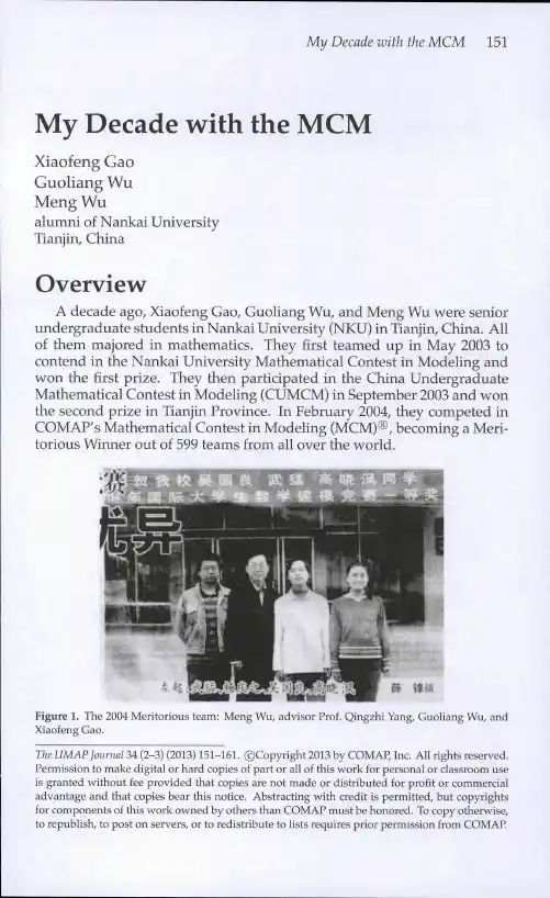
2010年美赛论文写作整理7273的o 奖论文Title Tracking serial criminals with a road metric 目的ing with 模型名称模型名称Abstract 句型整理句型整理Present a model to 什么目的什么目的 based on 什么数据什么数据We first create 自己建立的模型的名称自己建立的模型的名称 in order to 这个模型的功能这个模型的功能这个模型的功能 We apply 资料上的高端模型名称资料上的高端模型名称 with our 自己建立的模型名称, which allows us to 什么目的什么目的In In order order order to to 什么目的,we we use use use a a a refinement refinement refinement of of of a a a model model model developed developed developed by by 谁提出的, adapting it to the 自己建立的模型的名称自己建立的模型的名称This This method method method developed developed 模型里的什么东西模型里的什么东西 for 什么目的什么目的 by 什么方法或者理由依据依据We apply our model to 案例s ,blahblahblah Our model was successful in 什么目的,and might prove useful in 那个领域那个领域行文方法行文方法 1.自己给模型起了一个名字.自己给模型起了一个名字2.然后不停地说为了干什么,我们的模型怎么样怎么样(改进了前人的,用前人的检验了之类的)人的检验了之类的)3.模型运用在那些实例上,取得了怎样的效果//并没有具体的说运算的结果,只是说模型很成功。
TheUMAP JournalPublisherCOMAP ,Inc.Vol.31,No.2Executive PublisherSolomon A.GarfunkelILAP EditorChris ArneyDept.of Math’l Sciencesitary AcademyWest Point,NY 10996david.arney@On Jargon EditorYves NievergeltDept.of MathematicsEastern Washington Univ.Cheney,WA 99004ynievergelt@Reviews EditorJames M.CargalMathematics Dept.Troy University—Montgomery Campus231Montgomery St.Montgomery,AL 36104jmcargal@Chief Operating Of ficerLaurie W.Arag´onProduction ManagerGeorge WardCopy EditorJulia CollinsDistributionJohn Tomicek Editor Paul J.Campbell Beloit College 700College St.Beloit,WI 53511–5595campbell@ Associate Editors Don Adolphson Chris Arney Aaron Archer Ron Barnes Arthur Benjamin Robert Bosch James M.Cargal Murray K.Clayton Lisette De Pillis James P .Fink Solomon A.Garfunkel William B.Gearhart William C.Giauque Richard Haberman Jon Jacobsen Walter Meyer Yves Nievergelt Michael O’Leary Catherine A.Roberts John S.Robertson Philip D.Straf fin J.T.Sutcliffe Brigham Young Univ.Army Research Of fice AT&T Shannon b.U.of Houston—Downtn Harvey Mudd College Oberlin College Troy U.—Montgomery U.of Wisc.—Madison Harvey Mudd College Gettysburg College COMAP ,Inc.Calif.State U.,Fullerton Brigham Young Univ.Southern Methodist U.Harvey Mudd College Adelphi University Eastern Washington U.Towson University College of the Holy Cross Georgia Military College Beloit College St.Mark’s School,DallasSubscription Rates for 2010 Calendar Year: Volume 31Institutional Web Memberships do not provide print materials. Web memberships allow members to search our online catalog, download COMAP print materials, and reproduce them for classroom use.(Domestic) #3030 $467 (Outside U.S.) #3030 $467Institutional Memberships receive print copies of The UMAP Journal quarterly, our annual CD collection UMAP Modules, Tools for Teaching, and our organizational newsletter Consortium.(Domestic) #3040 $312 (Outside U.S.) #3041 $351Institutional Plus Memberships receive print copies of the quarterly issues of The UMAP Journal, our annual CD collection UMAP Modules, Tools for Teaching, our organizational newsletter Consortium, and online membership that allows members to search our online catalog, download COMAP print materials, and reproduce them for classroom use.(Domestic) #3070 $615 (Outside U.S.) #3071 $659For individual membership options visit for more information.To order, send a check or money order to COMAP, or call toll-free1-800-77-COMAP (1-800-772-6627).The UMAP Journal is published quarterly by the Consortium for Mathematics and Its Applications (COMAP), Inc., Suite 3B, 175 Middlesex Tpke.,Bedford, MA, 01730, in coop-eration with the American Mathematical Association of Two-Y ear Colleges (AMATY C), the Mathematical Association of America (MAA), the National Council of Teachers of Mathematics (NCTM), the American Statistical Association (ASA), the Society for Industrial and Applied Mathematics (SIAM), and The Institute for Operations Re-search and the Management Sciences (INFORMS). The Journal acquaints readers with a wide variety of professional applications of the mathematical sciences and provides a forum for the discussion of new directions in mathematical education (ISSN 0197-3622).Periodical rate postage paid at Boston, MA and at additional mailing offices.Send address changes to: info@COMAP, Inc., Suite 3B, 175 Middlesex Tpke., Bedford, MA, 01730© Copyright 2010 by COMAP, Inc. All rights reserved.Mathematical Contest in Modeling (MCM)®, High School Mathematical Contest in Modeling (HiMCM)®, and Interdisciplinary Contest in Modeling(ICM)®are registered trade marks of COMAP, Inc.Vol.31,No.22010Table of ContentsEditorialThe Modeling Contests in2010Paul J.Campbell (93)MCM Modeling ForumResults of the2010Mathematical Contest in ModelingFrank R.Giordano (95)The Sweet Spot:A Wave Model of Baseball BatsYang Mou,Peter Diao,and Rajib Quabili (105)Judges’Commentary:The Outstanding Sweet Spot Papers Michael Tortorella (123)Centroids,Clusters,and Crime:Anchoring the Geographic Profiles of Serial CriminalsAnil S.Damle,Colin G.West,and Eric J.Benzel (129)Judges’Commentary:The Outstanding Geographic Profiling Papers Marie Vanisko (149)Judges’Commentary:The Fusaro Award for theGeographic Profiling ProblemMarie Vanisko and Peter Anspach (153)ICM Modeling ForumResults of the2010Interdisciplinary Contest in ModelingChris Arney (157)Shedding Light on Marine PollutionBrittany Harris,Chase Peaslee,and Kyle Perkins (165)Author’s Commentary:The Marine Pollution ProblemMiriam C.Goldstein (175)Judges’Commentary:The Outstanding Marine Pollution Papers Rodney Sturdivant (179)Editorial93EditorialThe2010Modeling ContestsPaul J.CampbellMathematics and Computer ScienceBeloit CollegeBeloit,WI53511–5595campbell@BackgroundBased on Ben Fusaro’s suggestion for an“applied Putnam”contest,in 1985COMAP introduced the Mathematical Contest in Modeling(MCM)R . Since then,this Journal has devoted an issue each year to the Outstanding contest papers.Even after substantial editing,that issue has sometimes run to more than three times the size of an ordinary issue.From2005through 2009,some papers appeared in electronic form only.The2,254MCM teams in2010was almost double the number in2008.Also,since the introduction in1999of the Interdisciplinary Contest in Modeling(ICM)R (which has separate funding and sponsorship from the MCM),the Journal has devoted a second of its four annual issues to Out-standing papers from that contest.A New Designation for PapersIt has become increasingly difficult to identify just a handful of Out-standing papers for each problem.After14Outstanding MCM teams in 2007,there have been9in each year since,despite more teams competing.The judges have been overwhelmed by increasing numbers of Merito-rious papers from which to select the truly Outstanding.As a result,this year there is a new designation of Finalist teams,between Outstanding and Meritorious.It recognizes the less than1%of papers that reached thefinal (seventh)round of judging but were not selected as Outstanding.Each Finalist paper displayed some modeling that distinguished it from the rest of the Meritorious papers.We think that the Finalist papers deserve special The UMAP Journal31(2)(2010)93–94.c Copyright2010by COMAP,Inc.All rights reserved. Permission to make digital or hard copies of part or all of this work for personal or classroom use is granted without fee provided that copies are not made or distributed for profit or commercial advantage and that copies bear this notice.Abstracting with credit is permitted,but copyrights for components of this work owned by others than COMAP must be honored.To copy otherwise, to republish,to post on servers,or to redistribute to lists requires prior permission from COMAP.94The UMAP Journal31.2(2010)recognition,and the mathematical professional societies are investigating ways to recognize the Finalist papers.Just One Contest Issue Each YearTaking up two of the four Journal issues each year,and sometimes two-thirds of the pages,the amount of material from the two contests has come to overbalance the other content of the Journal.The Executive Publisher,Sol Garfunkel,and I have decided to return more of the Journal to its original purpose,as set out30years ago,to: acquaint readers with a wide variety of professional applications of the mathematical sciences,and provide a forum for discussions of new directions in mathematical education.[Finney and Garfunkel1980,2–3] Henceforth,we plan to devote just a single issue of the Journal each year to the two contests combined.That issue—this issue—will appear during the summer and contain•reports on both contests,including the problem statements and names of the Outstanding teams and their members;•authors’,judges’,and practitioners’commentaries(as available)on the problems and the Outstanding papers;and•just one Outstanding paper from each problem.Available separately from COMAP on a CD-ROM very soon after the contests(as in2009and again this year)will be:•full original versions of all of the Outstanding papers,and•full results for all teams.Your RoleThe ever-increasing engagement of students in the contests has been astonishing;the steps above help us to cope with this success.There will now be more room in the Journal for material on mathemati-cal modeling,applications of mathematics,and ideas and perspectives on mathematics education at the collegiate level—articles,UMAP Modules, Minimodules,ILAP Modules,guest editorials.We look forward to your contribution.ReferenceFinney,Ross L.,and Solomon Garfunkel.1980.UMAP and The UMAP Jour-nal.The UMAP Journal0:1–4.Results of the2010MCM95 Modeling ForumResults of the2010Mathematical Contest in Modeling Frank R.Giordano,MCM DirectorNaval Postgraduate School1University CircleMonterey,CA93943–5000frgiorda@IntroductionA total of2,254teams of undergraduates from hundreds of institutions and departments in14countries,spent a weekend in February working on applied mathematics problems in the26th Mathematical Contest in Modeling(MCM)R .The2010MCM began at8:00P.M.EST on Thursday,February18,and ended at8:00P.M.EST on Monday,February22.During that time,teams of up to three undergraduates researched,modeled,and submitted a solution to one of two open-ended modeling problems.Students registered,obtained contest materials,downloaded the problem and data,and entered completion data through COMAP’s MCM Website.After a weekend of hard work,solution papers were sent to COMAP on Monday.Two of the top papers appear in this issue of The UMAP Journal,together with commentaries.In addition to this special issue of The UMAP Journal,COMAP has made available a special supplementary2010MCM-ICM CD-ROM containing the press releases for the two contests,the results,the problems,and original ver-sions of the Outstanding rmation about ordering the CD-ROM is at /product/cdrom/index.html or from(800) 772–6627.Results and winning papers from thefirst25contests were published in special issues of Mathematical Modeling(1985–1987)and The UMAP Journal (1985–2009).The1994volume of Tools for Teaching,commemorating the tenth anniversary of the contest,contains the20problems used in thefirst10years of the contest and a winning paper for each year.That volume and the special The UMAP Journal31(2)(2010)95–104.c Copyright2010by COMAP,Inc.All rights reserved. Permission to make digital or hard copies of part or all of this work for personal or classroom use is granted without fee provided that copies are not made or distributed for profit or commercial advantage and that copies bear this notice.Abstracting with credit is permitted,but copyrights for components of this work owned by others than COMAP must be honored.To copy otherwise, to republish,to post on servers,or to redistribute to lists requires prior permission from COMAP.96The UMAP Journal31.2(2010)MCM issues of the Journal for the last few years are available from COMAP.The 1994volume is also available on COMAP’s special Modeling Resource CD-ROM. Also available is The MCM at21CD-ROM,which contains the20problems from the second10years of the contest,a winning paper from each year,and advice from advisors of Outstanding teams.These CD-ROMs can be ordered from COMAP at /product/cdrom/index.html.This year,the two MCM problems represented significant challenges:•Problem A,“The Sweet Spot,”asked teams to explain why the spot on a baseball bat where maximum power is transferred to the ball is not at the end of the bat and to determine whether“corking”a bat(hollowing it out and replacing the hardwood with cork)enhances the“sweet spot”effect.•Problem B,“Criminology,”asked teams to develop geographical profiling to aid police infinding serial criminals.In addition to the MCM,COMAP also sponsors the Interdisciplinary Con-test in Modeling(ICM)R and the High School Mathematical Contest in Mod-eling(HiMCM)R :•The ICM runs concurrently with MCM and for the next several years will offer a modeling problem involving an environmental topic.Results of this year’s ICM are on the COMAP Website at / undergraduate/contests.The contest report,an Outstanding paper,and commentaries appear in this issue.•The HiMCM offers high school students a modeling opportunity similar to the MCM.Further details about the HiMCM are at ap.com/highschool/contests.2010MCM Statistics•2,254teams participated•15high school teams(<1%)•358U.S.teams(21%)•1,890foreign teams(79%),from Australia,Canada,China,Finland,Ger-many,Indonesia,Ireland,Jamaica,Malaysia,Pakistan,Singapore,South Africa,United Kingdom•9Outstanding Winners(<0.5%)•12Finalists(0.5%)•431Meritorious Winners(19%)•542Honorable Mentions(24%)•1,245Successful Participants(55%)Results of the2010MCM97Problem A:The Sweet SpotExplain the“sweet spot”on a baseball bat.Every hitter knows that there is a spot on the fat part of a baseball bat where maximum power is transferred to the ball when hit.Why isn’t this spot at the end of the bat?A simple explanation based on torque might seem to identify the end of the bat as the sweet spot,but this is known to be empirically incorrect.Develop a model that helps explain this empiricalfinding.Some players believe that“corking”a bat(hollowing out a cylinder in the head of the bat andfilling it with cork or rubber,then replacing a wood cap) enhances the“sweet spot”effect.Augment your model to confirm or deny this effect.Does this explain why Major League Baseball prohibits“corking”?Does the material out of which the bat is constructed matter?That is,does this model predict different behavior for wood(usually ash)or metal(usually aluminum)bats?Is this why Major League Baseball prohibits metal bats? Problem B:CriminologyIn1981,Peter Sutcliffe was convicted of13murders and subjecting a number of other people to vicious attacks.One of the methods used to narrow the search for Mr.Sutcliffe was tofind a“center of mass”of the locations of the attacks. In the end,the suspect happened to live in the same town predicted by this technique.Since that time,a number of more sophisticated techniques have been developed to determine the“geographical profile”of a suspected serial criminal based on the locations of the crimes.Your team has been asked by a local police agency to develop a method to aid in their investigations of serial criminals.The approach that you develop should make use of at least two different schemes to generate a geographical profile.You should develop a technique to combine the results of the different schemes and generate a useful prediction for law enforcement officers.The prediction should provide some kind of estimate or guidance about possible locations of the next crime based on the time and locations of the past crime scenes.If you make use of any other evidence in your estimate,you must provide specific details about how you incorporate the extra information.Your method should also provide some kind of estimate about how reliable the estimate will be in a given situation,including appropriate warnings.In addition to the required one-page summary,your report should include an additional two-page executive summary.The executive summary should provide a broad overview of the potential issues.It should provide an overview of your approach and describe situations when it is an appropriate tool and situations in which it is not an appropriate tool.The executive summary will be read by a chief of police and should include technical details appropriate to the intended audience.98The UMAP Journal31.2(2010)The ResultsThe solution papers were coded at COMAP headquarters so that names and affiliations of the authors would be unknown to the judges.Each paper was then read preliminarily by two“triage”judges at either Appalachian State University(Sweet Spot Problem)or at the National Security Agency(Crimi-nology Problem).At the triage stage,the summary and overall organization are the basis for judging a paper.If the judges’scores diverged for a paper,the judges conferred;if they still did not agree,a third judge evaluated the paper.AdditionalRegional Judging sites were created at the itary Academy and at the Naval Postgraduate School to support the growing number of contest submissions.Final judging took place at the Naval Postgraduate School,Monterey,CA. The judges classified the papers as follows:Honorable SuccessfulOutstanding Finalist Meritorious Mention Participation Total Sweet Spot Problem45180217533939 Criminology Problem57251325712130091243154212452239 We list here the9teams that the judges designated as Outstanding;the list of all participating schools,advisors,and results is at the COMAP Website.Outstanding TeamsInstitution and Advisor Team MembersSweet Spot Problem“An Optimal Model of‘Sweet Spot’Effect”Huazhong University of Science andTechnology Wuhan,Hubei,China Liang Gao Zhe Xiong Qipei Mei Fei Han“The Sweet Spot:A Wave Model of Baseball Bats”Princeton University Princeton,NJ Robert Calderbank Yang Mou Peter Diao Rajib QuabiliResults of the2010MCM99“Brody Power Model:An Analysis of Baseball’s‘Sweet Spot’”itary Academy West Point,NY Elizabeth Schott David CovellBen Garlick Chandler Williams“An Identification of‘Sweet Spot’”Zhejiang University Hangzhou,China Xinxin XuCong ZhaoYuguang YangZuogong Yue Criminology Papers“Predicting a Serial Criminal’s Next Crime Location Using Geographic Profiling”Bucknell University Lewisburg,PA Nathan C.Ryan Bryan Ward Ryan Ward Dan Cavallaro“Following the Trail of Data”Rensselaer Polytechnic Institute Troy,NYPeter R.Kramer Yonatan Naamad Joseph H.Gibney Emily P.Meissen“From Kills to Kilometers:Using Centrographic Techniques and Rational Choice Theory forGeographical Profiling of Serial Killers”Tufts University Medford,MA Scott MacLachlan Daniel Brady Liam Clegg Victor Minden“Centroids,Clusters,and Crime:Anchoring the Geographic Profile of Serial Criminals”University of Colorado—Boulder Boulder,COAnne M.Dougherty Anil S.Damle Colin G.West Eric J.Benzel“Tracking Serial Criminals with a Road Metric”University of Washington Seattle,WAJames Allen Morrow Ian Zemke Mark Bun Jerry Li100The UMAP Journal31.2(2010)Awards and ContributionsEach participating MCM advisor and team member received a certificate signed by the Contest Director and the appropriate Head Judge.INFORMS,the Institute for Operations Research and the Management Sciences,recognized the teams from Princeton University(Sweet Spot Prob-lem)and Tufts University(Criminology Problem)as INFORMS Outstand-ing teams and provided the following recognition:•a letter of congratulations from the current president of INFORMS to each team member and to the faculty advisor;•a check in the amount of$300to each team member;•a bronze plaque for display at the team’s institution,commemorating team members’achievement;•individual certificates for team members and faculty advisor as a per-sonal commemoration of this achievement;and•a one-year student membership in INFORMS for each team member, which includes their choice of a professional journal plus the OR/MS Today periodical and the INFORMS newsletter.The Society for Industrial and Applied Mathematics(SIAM)designated one Outstanding team from each problem as a SIAM Winner.The teams were from Huazhong University of Science and Technology(Sweet Spot Problem)and Rensselaer PolytechnicInstitute(CriminologyProblem).Each of the team members was awarded a$300cash prize,and the teams received partial expenses to present their results in a special Minisymposium at the SIAM Annual Meeting in Pittsburgh,PA in July.Their schools were given a framed hand-lettered certificate in gold leaf.The Mathematical Association of America(MAA)designated one Out-standing North American team from each problem as an MAA Winner. The teams were from the itary Academy(Sweet Spot Problem)and the University of Colorado—Boulder(Criminology Problem).With partial travel support from the MAA,the teams presented their solution at a spe-cial session of the MAA Mathfest in Pittsburgh,PA in August.Each team member was presented a certificate by an official of the MAA Committee on Undergraduate Student Activities and Chapters.Ben Fusaro AwardOne Meritorious or Outstanding paper was selected for each problem for the Ben Fusaro Award,named for the Founding Director of the MCM and awarded for the seventh time this year.It recognizes an especially creative approach;details concerning the award,its judging,and Ben Fusaro are inResults of the2010MCM101 Vol.25(3)(2004):195–196.The Ben Fusaro Award winners were Prince-ton University(Sweet Spot Problem)and Duke University(Criminology Problem).A commentary on the latter appears in this issue.JudgingDirectorFrank R.Giordano,Naval Postgraduate School,Monterey,CA Associate DirectorWilliam P.Fox,Dept.of Defense Analysis,Naval Postgraduate School, Monterey,CASweet Spot ProblemHead JudgeMarvin S.Keener,Executive Vice-President,Oklahoma State University, Stillwater,OKAssociate JudgesWilliam C.Bauldry,Chair,Dept.of Mathematical Sciences,Appalachian State University,Boone,NC(Head Triage Judge)Patrick J.Driscoll,Dept.of Systems Engineering,itary Academy, West Point,NY(INFORMS Judge)J.Douglas Faires,Youngstown State University,Youngstown,OHBen Fusaro,Dept.of Mathematics,Florida State University,Tallahassee,FL (SIAM Judge)Michael Jaye,Dept.of Mathematical Sciences,Naval Postgraduate School, Monterey,CAJohn L.Scharf,Mathematics Dept.,Carroll College,Helena,MT (MAA Judge)Michael Tortorella,Dept.of Industrial and Systems Engineering, Rutgers University,Piscataway,NJ(Problem Author)Richard Douglas West,Francis Marion University,Florence,SC Criminology ProblemHead JudgeMaynard Thompson,Mathematics Dept.,University of Indiana, Bloomington,INAssociate JudgesPeter Anspach,National Security Agency,Ft.Meade,MD(Head Triage Judge)Kelly Black,Mathematics Dept.,Union College,Schenectady,NY102The UMAP Journal31.2(2010)Jim Case(SIAM Judge)William P.Fox,Dept.of Defense Analysis,Naval Postgraduate School, Monterey,CAFrank R.Giordano,Naval Postgraduate School,Monterey,CAVeena Mendiratta,Lucent Technologies,Naperville,ILDavid H.Olwell,Naval Postgraduate School,Monterey,CAMichael O’Leary,Towson State University,Towson,MD(Problem Author) Kathleen M.Shannon,Dept.of Mathematics and Computer Science, Salisbury University,Salisbury,MD(MAA Judge)Dan Solow,Case Western Reserve University,Cleveland,OH (INFORMS Judge)Marie Vanisko,Dept.of Mathematics,Carroll College,Helena,MT (Ben Fusaro Award Judge)Regional Judging Session at itary AcademyHead JudgesPatrick J.Driscoll,Dept.of Systems Engineering,United States Military Academy(USMA),West Point,NYAssociate JudgesTim Elkins,Dept.of Systems Engineering,USMADarrall Henderson,Sphere Consulting,LLCSteve Horton,Dept.of Mathematical Sciences,USMATom Meyer,Dept.of Mathematical Sciences,USMAScott Nestler,Dept.of Mathematical Sciences,USMARegional Judging Session at Naval Postgraduate SchoolHead JudgesWilliam P.Fox,Dept.of Defense Analysis,Naval Postgraduate School, Monterey,CAFrank R. Giordano,Naval Postgraduate School,Monterey,CA Associate JudgesMatt Boensel,Robert Burks,Peter Gustaitis,Michael Jaye,and Greg Mislick —all from the Naval Postgraduate School,Monterey,CATriage Session for Sweet Spot ProblemHead Triage JudgeWilliam C.Bauldry,Chair,Dept.of Mathematical Sciences,Appalachian State University,Boone,NCAssociate JudgesJeffry Hirst,Greg Rhoads,and Kevin Shirley—all from Dept.of Mathematical Sciences,Appalachian State University, Boone,NCResults of the2010MCM103Triage Session for Criminology ProblemHead Triage JudgePeter Anspach,National Security Agency(NSA),Ft.Meade,MD Associate JudgesJim CaseOther judges from inside and outside NSA,who wish not to be named.Sources of the ProblemsThe Sweet Spot Problem was contributed by Michael Tortorella(Rutgers University),and the Criminology Problem by Michael O’Leary(Towson University)and Kelly Black(Clarkson University). AcknowledgmentsMajor funding for the MCM is provided by the National Security Agency (NSA)and by COMAP.Additional support is provided by the Institute for Operations Research and the Management Sciences(INFORMS),the Soci-ety for Industrial and Applied Mathematics(SIAM),and the Mathematical Association of America(MAA).We are indebted to these organizations for providing judges and prizes.We also thank for their involvement and support the MCM judges and MCM Board members for their valuable and unflagging efforts,as well as •Two Sigma Investments.(This group of experienced,analytical,and technicalfinancial professionals based in New York builds and operates sophisticated quantitative trading strategies for domestic and interna-tional markets.Thefirm is successfully managing several billion dol-lars using highly-automated trading technologies.For more information about Two Sigma,please visit .)•Jane Street Capital,LLC.(This proprietary tradingfirm operates around the clock and around the globe.“We bring a deep understanding of markets,a scientific approach,and innovative technology to bear on the problem of trading profitably in the world’s highly competitivefinancial markets,focusing primarily on equities and equity derivatives.Founded in2000,Jane Street employes over200people in offices in new York,Lon-don,and Tokyo.Our entrepreneurial culture is driven by our talented team of traders and programmers.”For more information about Jane Street Capital,please visit .)104The UMAP Journal31.2(2010)CautionsTo the reader of research journals:Usually a published paper has been presented to an audience,shown to colleagues,rewritten,checked by referees,revised,and edited by a jour-nal editor.Each paper here is the result of undergraduates working on a problem over a weekend.Editing(and usually substantial cutting)has taken place;minor errors have been corrected,wording altered for clarity or economy,and style adjusted to that of The UMAP Journal.The student authors have proofed the results.Please peruse their efforts in that context.To the potential MCM Advisor:It might be overpowering to encounter such output from a weekend of work by a small team of undergraduates,but these solution papers are highly atypical.A team that prepares and participates will have an enrich-ing learning experience,independent of what any other team does.COMAP’s MathematicalContest in Modeling and InterdisciplinaryCon-test in Modeling are the only international modeling contests in which students work in teams.Centering its educational philosophy on mathe-matical modeling,COMAP uses mathematical tools to explore real-world problems.It serves the educational community as well as the world of work by preparing students to become better-informed and better-prepared citi-zens.Editor’s NoteThe complete roster of participating teams and results has become too long to reproduce in the printed copy of the Journal.It can now be found at the COMAP Website,in separatefiles for each problem:/undergraduate/contests/mcm/contests/ 2010/results/2010_MCM_Problem_A.pdf/undergraduate/contests/mcm/contests/ 2010/results/2010_MCM_Problem_B.pdf。
Number of People Entered Shanghai World Expo ParkAbstract:Key words:Contents1. Introduction (3)1.1 Why does toll way collects toll? (3)1.2 Toll modes (3)1.3 Toll collection methods (3)1.4 Annoyance in toll plazas (3)1.5 The origin of the toll way problem (3)1.6 Queuing theory (4)2. The Description of Problem (5)2.1 How do we approximate the whole course of paying toll? (5)2.2 How do we define the optimal configuration? (5)2.2.1 From the perspective of motorist (5)2.2.2 From the perspective of the toll plaza (6)2.2.3 Compromise (6)2.3 Overall optimization and local optimization (6)2.4 The differences in weights and sizes of vehicles (7)2.5 What if there is no data available? (7)3. Models (7)3.1 Basic Model (7)3.1.1 Symbols and Definitions (7)3.1.2 Assumptions (8)3.1.3 The Foundation of Model (9)3.1.4 Solution and Result (11)3.1.5 Analysis of the Result (11)3.1.6 Strength and Weakness (13)3.2 Improved Model (14)3.2.1 Extra Symbols (14)3.2.2 Additional Assumptions (14)3.2.3 The Foundation of Model (14)3.2.4 Solution and Result (15)3.2.5 Analysis of the Result (18)3.2.6 Strength and Weakness (19)4. Conclusions (19)4.1 Conclusions of the problem (19)4.2 Methods used in our models (19)4.3 Application of our models (19)5. Future Work (19)5.1 Another model (19)5.2 Another layout of toll plaza (23)5.3 The newly- adopted charging methods (23)6.References (23)7.Appendix (23)Programs and codes (24)I. IntroductionIn order to indicate the origin of the toll way problems, the following background is worth mentioning.1.11.21.31.41.51.6II. The Description of the Problem2.1 How do we approximate the whole course of paying toll?●●●●2.2 How do we define the optimal configuration?1) From the perspective of motorist:2) From the perspective of the toll plaza:3) Compromise:2.3 The local optimization and the overall optimization●●●Virtually:2.4 The differences in weights and sizes of vehicles2.5 What if there is no data available?III. Models3.1 Basic Model3.1.1 Terms, Definitions and SymbolsThe signs and definitions are mostly generated from queuing theory.●●●●●3.1.2 Assumptions●●●●●3.1.3 The Foundation of Model1) The utility function●The cost of toll plaza:●The loss of motorist:●The weight of each aspect:●Compromise:2) The integer programmingAccording to queuing theory, we can calculate the statistical properties as follows.3)The overall optimization and the local optimization●The overall optimization:●The local optimization:●The optimal number of tollbooths:3.1.4 Solution and Result1) The solution of the integer programming:2) Results:3.1.5 Analysis of the Result●Local optimization and overall optimization:●Sensitivity: The result is quite sensitive to the change of the threeparameters●Trend:●Comparison:3.1.6 Strength and Weakness●Strength: In despite of this, the model has proved that . Moreover, wehave drawn some useful conclusions about . T he model is fit for, such as●Weakness: This model just applies to . As we have stated, . That’sjust what we should do in the improved model.3.2 Improved Model3.2.1 Extra SymbolsSigns and definitions indicated above are still valid. Here are some extra signs and definitions.●●●●3.2.2 Additional Assumptions●●●Assumptions concerning the anterior process are the same as the Basic Model.3.2.3 The Foundation of Model1) How do we determine the optimal number?As we have concluded from the Basic Model,3.2.4 Solution and Result1) Simulation algorithmBased on the analysis above, we design our simulation arithmetic as follows.●Step1:●Step2:●Step3:●Step4:●Step5:●Step6:●Step7:●Step8:●Step9:2) Flow chartThe figure below is the flow chart of the simulation.3) Solution3.2.5 Analysis of the Result3.2.6 Strength and Weakness●Strength: The Improved Model aims to make up for the neglect of .The result seems to declare that this model is more reasonable than the Basic Model and much more effective than the existing design.●Weakness: . Thus the model is still an approximate on a large scale. Thishas doomed to limit the applications of it.IV. Conclusions4.1 Conclusions of the problem●●●4.2 Methods used in our models●●●4.3 Applications of our models●●●V. Future Work5.1 Another model5.1.1The limitations of queuing theory 5.1.25.1.35.1.41)●●●●2)●●●3)●●●4)5.2 Another layout of toll plaza5.3 The newly- adopted charging methodsVI. References[1][2][3][4]VII. Appendix。
2008国际大学生数学建模比赛参赛作品---------WHO所属成员国卫生系统绩效评估作品名称:Less Resources, more outcomes参赛单位:重庆大学参赛时间:2008年2月15日至19日指导老师:何仁斌参赛队员:舒强机械工程学院05级罗双才自动化学院05级黎璨计算机学院05级ContentLess Resources, More Outcomes (4)1. Summary (4)2. Introduction (5)3. Key Terminology (5)4. Choosing output metrics for measuring health care system (5)4.1 Goals of Health Care System (6)4.2 Characteristics of a good health care system (6)4.3 Output metrics for measuring health care system (6)5. Determining the weight of the metrics and data processing (8)5.1 Weights from statistical data (8)5.2 Data processing (9)6. Input and Output of Health Care System (9)6.1 Aspects of Input (10)6.2 Aspects of Output (11)7. Evaluation System I : Absolute Effectiveness of HCS (11)7.1Background (11)7.2Assumptions (11)7.3Two approaches for evaluation (11)1. Approach A : Weighted Average Evaluation Based Model (11)2. Approach B: Fuzzy Comprehensive Evaluation Based Model [19][20] (12)7.4 Applying the Evaluation of Absolute Effectiveness Method (14)8. Evaluation system II: Relative Effectiveness of HCS (16)8.1 Only output doesn’t work (16)8.2 Assumptions (16)8.3 Constructing the Model (16)8.4 Applying the Evaluation of Relative Effectiveness Method (17)9. EAE VS ERE: which is better? (17)9.1 USA VS Norway (18)9.2 USA VS Pakistan (18)10. Less Resources, more outcomes (19)10.1Multiple Logistic Regression Model (19)10.1.1 Output as function of Input (19)10.1.2Assumptions (19)10.1.3Constructing the model (19)10.1.4. Estimation of parameters (20)10.1.5How the six metrics influence the outcomes? (20)10.2 Taking USA into consideration (22)10.2.1Assumptions (22)10.2.2 Allocation Coefficient (22)10.3 Scenario 1: Less expenditure to achieve the same goal (24)10.3.1 Objective function: (24)10.3.2 Constraints (25)10.3.3 Optimization model 1 (25)10.3.4 Solutions of the model (25)10.4. Scenario2: More outcomes with the same expenditure (26)10.4.1Objective function (26)10.4.2Constraints (26)10.4.3 Optimization model 2 (26)10.4.4Solutions to the model (27)15. Strengths and Weaknesses (27)Strengths (27)Weaknesses (27)16. References (28)Less Resources, More Outcomes1. SummaryIn this paper, we regard the health care system (HCS) as a system with input and output, representing total expenditure on health and its goal attainment respectively. Our goal is to minimize the total expenditure on health to archive the same or maximize the attainment under given expenditure.First, five output metrics and six input metrics are specified. Output metrics are overall level of health, distribution of health in the population,etc. Input metrics are physician density per 1000 population, private prepaid plans as % private expenditure on health, etc.Second, to evaluate the effectiveness of HCS, two evaluation systems are employed in this paper:●Evaluation of Absolute Effectiveness(EAE)This evaluation system only deals with the output of HCS,and we define Absolute Total Score (ATS) to quantify the effectiveness. During the evaluation process, weighted average sum of the five output metrics is defined as ATS, and the fuzzy theory is also employed to help assess HCS.●Evaluation of Relative Effectiveness(ERE)This evaluation system deals with the output as well as its input, and also we define Relative Total Score (RTS) to quantify the effectiveness. The measurement to ATS is units of output produced by unit of input.Applying the two kinds of evaluation system to evaluate HCS of 34 countries (USA included), we can find some countries which rank in a higher position in EAE get a relatively lower rank in ERE, such as Norway and USA, indicating that their HCS should have been able to archive more under their current resources .Therefore, taking USA into consideration, we try to explore how the input influences the output and archive the goal: less input, more output. Then three models are constructed to our goal:●Multiple Logistic RegressionWe model the output as function of input by the logistic equation. In more detains, we model ATS (output) as the function of total expenditure on health system. By curve fitting, we estimate the parameters in logistic equation, and statistical test presents us a satisfactory result.●Linear Optimization Model on minimizing the total expenditure on healthWe try to minimize the total expenditure and at the same time archive the same, that is to get a ATS of 0.8116. We employ software to solve the model, and by the analysis of the results. We cut it to 2023.2 billion dollars, compared to the original data 2109.8 billion dollars.●Linear Optimization Model on maximizing the attainment. We try to maximize the attainment (absolute total score) under the same total expenditure in2007.And we optimize the ATS to 0.8823, compared to the original data 0.8116.Finally, we discuss strengths and weaknesses of our models and make necessary recommendations to the policy-makers。
Why Crime Doesn’t Pay:Locating Criminals Through Geographic ProfilingControl Number:#7272February22,2010AbstractGeographic profiling,the application of mathematics to criminology, has greatly improved police efforts to catch serial criminals byfinding their residence.However,many geographic profiles either generate an extremely large area for police to cover or generates regions that are unstable with respect to internal parameters of the model.We propose,formulate,and test the Gaussian Rossmooth(GRS)Method,which takes the strongest elements from multiple existing methods and combines them into a more stable and robust model.We also propose and test a model to predict the location of the next crime.We tested our models on the Yorkshire Ripper case.Our results show that the GRS Method accurately predicts the location of the killer’s residence.Additionally,the GRS Method is more stable with respect to internal parameters and more robust with respect to outliers than the existing methods.The model for predicting the location of the next crime generates a logical and reasonable region where the next crime may occur.We conclude that the GRS Method is a robust and stable model for creating a strong and effective model.1Control number:#72722Contents1Introduction4 2Plan of Attack4 3Definitions4 4Existing Methods54.1Great Circle Method (5)4.2Centrography (6)4.3Rossmo’s Formula (8)5Assumptions8 6Gaussian Rossmooth106.1Properties of a Good Model (10)6.2Outline of Our Model (11)6.3Our Method (11)6.3.1Rossmooth Method (11)6.3.2Gaussian Rossmooth Method (14)7Gaussian Rossmooth in Action157.1Four Corners:A Simple Test Case (15)7.2Yorkshire Ripper:A Real-World Application of the GRS Method167.3Sensitivity Analysis of Gaussian Rossmooth (17)7.4Self-Consistency of Gaussian Rossmooth (19)8Predicting the Next Crime208.1Matrix Method (20)8.2Boundary Method (21)9Boundary Method in Action21 10Limitations22 11Executive Summary2311.1Outline of Our Model (23)11.2Running the Model (23)11.3Interpreting the Results (24)11.4Limitations (24)12Conclusions25 Appendices25 A Stability Analysis Images252Control number:#72723List of Figures1The effect of outliers upon centrography.The current spatial mean is at the red diamond.If the two outliers in the lower leftcorner were removed,then the center of mass would be locatedat the yellow triangle (6)2Crimes scenes that are located very close together can yield illog-ical results for the spatial mean.In this image,the spatial meanis located at the same point as one of the crime scenes at(1,1)..7 3The summand in Rossmo’s formula(2B=6).Note that the function is essentially0at all points except for the scene of thecrime and at the buffer zone and is undefined at those points..9 4The summand in smoothed Rossmo’s formula(2B=6,φ=0.5, and EPSILON=0.5).Note that there is now a region aroundthe buffer zone where the value of the function no longer changesvery rapidly (13)5The Four Corners Test Case.Note that the highest hot spot is located at the center of the grid,just as the mathematics indicates.15 6Crimes and residences of the Yorkshire Ripper.There are two residences as the Ripper moved in the middle of the case.Someof the crime locations are assaults and others are murders (16)7GRS output for the Yorkshire Ripper case(B=2.846).Black dots indicate the two residences of the killer (17)8GRS method run on Yorkshire Ripper data(B=2).Note that the major difference between this model and Figure7is that thehot zones in thisfigure are smaller than in the original run (18)9GRS method run on Yorkshire Ripper data(B=4).Note that the major difference between this model and Figure7is that thehot zones in thisfigure are larger than in the original run (19)10The boundary region generated by our Boundary Method.Note that boundary region covers many of the crimes committed bythe Sutcliffe (22)11GRS Method onfirst eleven murders in the Yorkshire Ripper Case25 12GRS Method onfirst twelve murders in the Yorkshire Ripper Case263Control number:#727241IntroductionCatching serial criminals is a daunting problem for law enforcement officers around the world.On the one hand,a limited amount of data is available to the police in terms of crimes scenes and witnesses.However,acquiring more data equates to waiting for another crime to be committed,which is an unacceptable trade-off.In this paper,we present a robust and stable geographic profile to predict the residence of the criminal and the possible locations of the next crime.Our model draws elements from multiple existing models and synthesizes them into a unified model that makes better use of certain empirical facts of criminology.2Plan of AttackOur objective is to create a geographic profiling model that accurately describes the residence of the criminal and predicts possible locations for the next attack. In order to generate useful results,our model must incorporate two different schemes and must also describe possible locations of the next crime.Addi-tionally,we must include assumptions and limitations of the model in order to ensure that it is used for maximum effectiveness.To achieve this objective,we will proceed as follows:1.Define Terms-This ensures that the reader understands what we aretalking about and helps explain some of the assumptions and limitations of the model.2.Explain Existing Models-This allows us to see how others have at-tacked the problem.Additionally,it provides a logical starting point for our model.3.Describe Properties of a Good Model-This clarifies our objectiveand will generate a sketelon for our model.With this underlying framework,we will present our model,test it with existing data,and compare it against other models.3DefinitionsThe following terms will be used throughout the paper:1.Spatial Mean-Given a set of points,S,the spatial mean is the pointthat represents the middle of the data set.2.Standard Distance-The standard distance is the analog of standarddeviation for the spatial mean.4Control number:#727253.Marauder-A serial criminal whose crimes are situated around his or herplace of residence.4.Distance Decay-An empirical phenomenon where criminal don’t traveltoo far to commit their crimes.5.Buffer Area-A region around the criminal’s residence or workplacewhere he or she does not commit crimes.[1]There is some dispute as to whether this region exists.[2]In our model,we assume that the buffer area exists and we measure it in the same spatial unit used to describe the relative locations of other crime scenes.6.Manhattan Distance-Given points a=(x1,y1)and b=(x2,y2),theManhattan distance from a to b is|x1−x2|+|y1−y2|.This is also known as the1−norm.7.Nearest Neighbor Distance-Given a set of points S,the nearestneighbor distance for a point x∈S ismin|x−s|s∈S−{x}Any norm can be chosen.8.Hot Zone-A region where a predictive model states that a criminal mightbe.Hot zones have much higher predictive scores than other regions of the map.9.Cold Zone-A region where a predictive model scores exceptionally low. 4Existing MethodsCurrently there are several existing methods for interpolating the position of a criminal given the location of the crimes.4.1Great Circle MethodIn the great circle method,the distances between crimes are computed and the two most distant crimes are chosen.Then,a great circle is drawn so that both of the points are on the great circle.The midpoint of this great circle is then the assumed location of the criminal’s residence and the area bounded by the great circle is where the criminal operates.This model is computationally inexpensive and easy to understand.[3]Moreover,it is easy to use and requires very little training in order to master the technique.[2]However,it has certain drawbacks.For example,the area given by this method is often very large and other studies have shown that a smaller area suffices.[4]Additionally,a few outliers can generate an even larger search area,thereby further slowing the police effort.5Control number:#727264.2CentrographyIn centrography ,crimes are assigned x and y coordinates and the “center of mass”is computed as follows:x center =n i =1x i ny center =n i =1y i nIntuitively,centrography finds the mean x −coordinate and the mean y -coordinate and associates this pair with the criminal’s residence (this is calledthe spatial mean ).However,this method has several flaws.First,it can be unstablewith respect to outliers.Consider the following set of points (shown in Figure 1:Figure 1:The effect of outliers upon centrography.The current spatial mean is at the red diamond.If the two outliers in the lower left corner were removed,then the center of mass would be located at the yellow triangle.Though several of the crime scenes (blue points)in this example are located in a pair of upper clusters,the spatial mean (red point)is reasonably far away from the clusters.If the two outliers are removed,then the spatial mean (yellow point)is located closer to the two clusters.A similar method uses the median of the points.The median is not so strongly affected by outliers and hence is a more stable measure of the middle.[3]6Control number:#72727 Alternatively,we can circumvent the stability problem by incorporating the 2-D analog of standard deviation called the standard distance:σSD=d center,iNwhere N is the number of crimes committed and d center,i is the distance from the spatial center to the i th crime.By incorporating the standard distance,we get an idea of how“close together”the data is.If the standard distance is small,then the kills are close together. However,if the standard distance is large,then the kills are far apart. Unfortunately,this leads to another problem.Consider the following data set (shown in Figure2):Figure2:Crimes scenes that are located very close together can yield illogical results for the spatial mean.In this image,the spatial mean is located at the same point as one of the crime scenes at(1,1).In this example,the kills(blue)are closely clustered together,which means that the centrography model will yield a center of mass that is in the middle of these crimes(in this case,the spatial mean is located at the same point as one of the crimes).This is a somewhat paradoxical result as research in criminology suggests that there is a buffer area around a serial criminal’s place of residence where he or she avoids the commission of crimes.[3,1]That is,the potential kill area is an annulus.This leads to Rossmo’s formula[1],another mathematical model that predicts the location of a criminal.7Control number:#727284.3Rossmo’s FormulaRossmo’s formula divides the map of a crime scene into grid with i rows and j columns.Then,the probability that the criminal is located in the box at row i and column j isP i,j=kTc=1φ(|x i−x c|+|y j−y c|)f+(1−φ)(B g−f)(2B−|x i−x c|−|y j−y c|)gwhere f=g=1.2,k is a scaling constant(so that P is a probability function), T is the total number of crimes,φputs more weight on one metric than the other,and B is the radius of the buffer zone(and is suggested to be one-half the mean of the nearest neighbor distance between crimes).[1]Rossmo’s formula incorporates two important ideas:1.Criminals won’t travel too far to commit their crimes.This is known asdistance decay.2.There is a buffer area around the criminal’s residence where the crimesare less likely to be committed.However,Rossmo’s formula has two drawbacks.If for any crime scene x c,y c,the equality2B=|x i−x c|+|y j−y c|,is satisfied,then the term(1−φ)(B g−f)(2B−|x i−x c|−|y j−y c|)gis undefined,as the denominator is0.Additionally,if the region associated withij is the same region as the crime scene,thenφi c j c is unde-fined by the same reasoning.Figure3illustrates this:This“delta function-like”behavior is disconcerting as it essentially states that the criminal either lives right next to the crime scene or on the boundary defined by Rossmo.Hence,the B-value becomes exceptionally important and needs its own heuristic to ensure its accuracy.A non-optimal choice of B can result in highly unstable search zones that vary when B is altered slightly.5AssumptionsOur model is an expansion and adjustment of two existing models,centrography and Rossmo’s formula,which have their own underlying assumptions.In order to create an effective model,we will make the following assumptions:1.The buffer area exists-This is a necessary assumption and is the basisfor one of the mathematical components of our model.2.More than5crimes have occurred-This assumption is importantas it ensures that we have enough data to make an accurate model.Ad-ditionally,Rossmo’s model stipulates that5crimes have occurred[1].8Control number:#72729Figure3:The summand in Rossmo’s formula(2B=6).Note that the function is essentially0at all points except for the scene of the crime and at the buffer zone and is undefined at those points3.The criminal only resides in one location-By this,we mean thatthough the criminal may change residence,he or she will not move toa completely different area and commit crimes there.Empirically,thisassumption holds,with a few exceptions such as David Berkowitz[1].The importance of this assumption is it allows us to adapt Rossmo’s formula and the centrography model.Both of these models implicitly assume that the criminal resides in only one general location and is not nomadic.4.The criminal is a marauder-This assumption is implicitly made byRossmo’s model as his spatial partition method only considers a small rectangular region that contains all of the crimes.With these assumptions,we present our model,the Gaussian Rossmooth method.9Control number:#7272106Gaussian Rossmooth6.1Properties of a Good ModelMuch of the literature regarding criminology and geographic profiling contains criticism of existing models for catching criminals.[1,2]From these criticisms, we develop the following criteria for creating a good model:1.Gives an accurate prediction for the location of the criminal-This is vital as the objective of this model is to locate the serial criminal.Obviously,the model cannot give a definite location of the criminal,but it should at least give law enforcement officials a good idea where to look.2.Provides a good estimate of the location of the next crime-Thisobjective is slightly harder than thefirst one,as the criminal can choose the location of the next crime.Nonetheless,our model should generate a region where law enforcement can work to prevent the next crime.3.Robust with respect to outliers-Outliers can severely skew predic-tions such as the one from the centrography model.A good model will be able to identify outliers and prevent them from adversely affecting the computation.4.Consitent within a given data set-That is,if we eliminate data pointsfrom the set,they do not cause the estimation of the criminal’s location to change excessively.Additionally,we note that if there are,for example, eight murders by one serial killer,then our model should give a similar prediction of the killer’s residence when it considers thefirstfive,first six,first seven,and all eight murders.5.Easy to compute-We want a model that does not entail excessivecomputation time.Hence,law enforcement will be able to get their infor-mation more quickly and proceed with the case.6.Takes into account empirical trends-There is a vast amount ofempirical data regarding serial criminals and how they operate.A good model will incorporate this data in order to minimize the necessary search area.7.Tolerates changes in internal parameters-When we tested Rossmo’sformula,we found that it was not very tolerant to changes of the internal parameters.For example,varying B resulted in substantial changes in the search area.Our model should be stable with respect to its parameters, meaning that a small change in any parameter should result in a small change in the search area.10Control number:#7272116.2Outline of Our ModelWe know that centrography and Rossmo’s method can both yield valuable re-sults.When we used the mean and the median to calculate the centroid of a string of murders in Yorkshire,England,we found that both the median-based and mean-based centroid were located very close to the home of the criminal. Additionally,Rossmo’s method is famous for having predicted the home of a criminal in Louisiana.In our approach to this problem,we adapt these methods to preserve their strengths while mitigating their weaknesses.1.Smoothen Rossmo’s formula-While the theory behind Rossmo’s for-mula is well documented,its implementation isflawed in that his formula reaches asymptotes when the distance away from a crime scene is0(i.e.point(x i,y j)is a crime scene),or when a point is exactly2B away froma crime scene.We must smoothen Rossmo’s formula so that idea of abuffer area is mantained,but the asymptotic behavior is removed and the tolerance for error is increased.2.Incorporate the spatial mean-Using the existing crime scenes,we willcompute the spatial mean.Then,we will insert a Gaussian distribution centered at that point on the map.Hence,areas near the spatial mean are more likely to come up as hot zones while areas further away from the spatial mean are less likely to be viewed as hot zones.This ensures that the intuitive idea of centrography is incorporated in the model and also provides a general area to search.Moreover,it mitigates the effect of outliers by giving a probability boost to regions close to the center of mass,meaning that outliers are unlikely to show up as hot zones.3.Place more weight on thefirst crime-Research indicates that crimi-nals tend to commit theirfirst crime closer to their home than their latter ones.[5]By placing more weight on thefirst crime,we can create a model that more effectively utilizes criminal psychology and statistics.6.3Our Method6.3.1Rossmooth MethodFirst,we eliminated the scaling constant k in Rossmo’s equation.As such,the function is no longer a probability function but shows the relative likelihood of the criminal living in a certain sector.In order to eliminate the various spikes in Rossmo’s method,we altered the distance decay function.11Control number:#727212We wanted a distance decay function that:1.Preserved the distance decay effect.Mathematically,this meant that thefunction decreased to0as the distance tended to infinity.2.Had an interval around the buffer area where the function values wereclose to each other.Therefore,the criminal could ostensibly live in a small region around the buffer zone,which would increase the tolerance of the B-value.We examined various distance decay functions[1,3]and found that the func-tions resembled f(x)=Ce−m(x−x0)2.Hence,we replaced the second term in Rossmo’s function with term of the form(1−φ)×Ce−k(x−x0)2.Our modified equation was:E i,j=Tc=1φ(|x i−x c|+|y j−y c|)f+(1−φ)×Ce−(2B−(|x i−x c|+|y j−y c|))2However,this maintained the problematic region around any crime scene.In order to eliminate this problem,we set an EPSILON so that any point within EPSILON(defined to be0.5spatial units)of a crime scene would have a weighting of a constant cap.This prevented the function from reaching an asymptote as it did in Rossmo’s model.The cap was defined asCAP=φEPSILON fThe C in our modified Rossmo’s function was also set to this cap.This way,the two maximums of our modified Rossmo’s function would be equal and would be located at the crime scene and the buffer zone.12Control number:#727213This function yielded the following curve (shown in in Figure4),which fit both of our criteria:Figure 4:The summand in smoothed Rossmo’s formula (2B =6,φ=0.5,and EPSILON =0.5).Note that there is now a region around the buffer zone where the value of the function no longer changes very rapidly.At this point,we noted that E ij had served its purpose and could be replaced in order to create a more intuitive idea of how the function works.Hence,we replaced E i,j with the following sum:Tc =1[D 1(c )+D 2(c )]where:D 1(c )=min φ(|x i −x c |+|y j −y c |),φEPSILON D 2(c )=(1−φ)×Ce −(2B −(|x i −x c |+|y j −y c |))2For equal weighting on both D 1(c )and D 2(c ),we set φto 0.5.13Control number:#7272146.3.2Gaussian Rossmooth MethodNow,in order to incorporate the inuitive method,we used centrography to locate the center of mass.Then,we generated a Gaussian function centered at this point.The Gaussian was given by:G=Ae −@(x−x center)22σ2x+(y−y center)22σ2y1Awhere A is the amplitude of the peak of the Gaussian.We determined that the optimal A was equal to2times the cap defined in our modified Rossmo’s equation.(A=2φEPSILON f)To deal with empirical evidence that thefirst crime was usually the closest to the criminal’s residence,we doubled the weighting on thefirst crime.However, the weighting can be represented by a constant,W.Hence,ourfinal Gaussian Rosmooth function was:GRS(x i,y j)=G+W(D1(1)+D2(1))+Tc=2[D1(c)+D2(c)]14Control number:#7272157Gaussian Rossmooth in Action7.1Four Corners:A Simple Test CaseIn order to test our Gaussain Rossmooth(GRS)method,we tried it against a very simple test case.We placed crimes on the four corners of a square.Then, we hypothesized that the model would predict the criminal to live in the center of the grid,with a slightly higher hot zone targeted toward the location of the first crime.Figure5shows our results,whichfits our hypothesis.Figure5:The Four Corners Test Case.Note that the highest hot spot is located at the center of the grid,just as the mathematics indicates.15Control number:#727216 7.2Yorkshire Ripper:A Real-World Application of theGRS MethodAfter the model passed a simple test case,we entered the data from the Yorkshire Ripper case.The Yorkshire Ripper(a.k.a.Peter Sutcliffe)committed a string of13murders and several assaults around Northern England.Figure6shows the crimes of the Yorkshire Ripper and the locations of his residence[1]:Figure6:Crimes and residences of the Yorkshire Ripper.There are two res-idences as the Ripper moved in the middle of the case.Some of the crime locations are assaults and others are murders.16Control number:#727217 When our full model ran on the murder locations,our data yielded the image show in Figure7:Figure7:GRS output for the Yorkshire Ripper case(B=2.846).Black dots indicate the two residences of the killer.In this image,hot zones are in red,orange,or yellow while cold zones are in black and blue.Note that the Ripper’s two residences are located in the vicinity of our hot zones,which shows that our model is at least somewhat accurate. Additionally,regions far away from the center of mass are also blue and black, regardless of whether a kill happened there or not.7.3Sensitivity Analysis of Gaussian RossmoothThe GRS method was exceptionally stable with respect to the parameter B. When we ran Rossmo’s model,we found that slight variations in B could create drastic variations in the given distribution.On many occassions,a change of 1spatial unit in B caused Rossmo’s method to destroy high value regions and replace them with mid-level value or low value regions(i.e.,the region would completely dissapper).By contrast,our GRS method scaled the hot zones.17Control number:#727218 Figures8and9show runs of the Yorkshire Ripper case with B-values of2and 4respectively.The black dots again correspond to the residence of the criminal. The original run(Figure7)had a B-value of2.846.The original B-value was obtained by using Rossmo’s nearest neighbor distance metric.Note that when B is varied,the size of the hot zone varies,but the shape of the hot zone does not.Additionally,note that when a B-value gets further away from the value obtained by the nearest neighbor distance metric,the accuracy of the model decreases slightly,but the overall search areas are still quite accurate.Figure8:GRS method run on Yorkshire Ripper data(B=2).Note that the major difference between this model and Figure7is that the hot zones in this figure are smaller than in the original run.18Control number:#727219Figure9:GRS method run on Yorkshire Ripper data(B=4).Note that the major difference between this model and Figure7is that the hot zones in this figure are larger than in the original run.7.4Self-Consistency of Gaussian RossmoothIn order to test the self-consistency of the GRS method,we ran the model on thefirst N kills from the Yorkshire Ripper data,where N ranged from6to 13,inclusive.The self-consistency of the GRS method was adversely affected by the center of mass correction,but as the case number approached11,the model stabilized.This phenomenon can also be attributed to the fact that the Yorkshire Ripper’s crimes were more separated than those of most marauders.A selection of these images can be viewed in the appendix.19Control number:#7272208Predicting the Next CrimeThe GRS method generates a set of possible locations for the criminal’s resi-dence.We will now present two possible methods for predicting the location of the criminal’s next attack.One method is computationally expensive,but more rigorous while the other method is computationally inexpensive,but more intuitive.8.1Matrix MethodGiven the parameters of the GRS method,the region analyzed will be a square with side length n spatial units.Then,the output from the GRS method can be interpreted as an n×n matrix.Hence,for any two runs,we can take the norm of their matrix difference and compare how similar the runs were.With this in mind,we generate the following method.For every point on the grid:1.Add crime to this point on the grid.2.Run the GRS method with the new set of crime points.pare the matrix generated with these points to the original matrix bysubtracting the components of the original matrix from the components of the new matrix.4.Take a matrix norm of this difference matrix.5.Remove the crime from this point on the grid.As a lower matrix norm indicates a matrix similar to our original run,we seek the points so that the matrix norm is minimized.There are several matrix norms to choose from.We chose the Frobenius norm because it takes into account all points on the difference matrix.[6]TheFrobenius norm is:||A||F=mi=1nj=1|a ij|2However,the Matrix Method has one serious drawback:it is exceptionally expensive to compute.Given an n×n matrix of points and c crimes,the GRS method runs in O(cn2).As the Matrix method runs the GRS method at each of n2points,we see that the Matrix Method runs in O(cn4).With the Yorkshire Ripper case,c=13and n=151.Accordingly,it requires a fairly long time to predict the location of the next crime.Hence,we present an alternative solution that is more intuitive and efficient.20Control number:#7272218.2Boundary MethodThe Boundary Method searches the GRS output for the highest point.Then,it computes the average distance,r,from this point to the crime scenes.In order to generate a resonable search area,it discards all outliers(i.e.,points that were several times further away from the high point than the rest of the crimes scenes.)Then,it draws annuli of outer radius r(in the1-norm sense)around all points above a certain cutoffvalue,defined to be60%of the maximum value. This value was chosen as it was a high enough percentage value to contain all of the hot zones.The beauty of this method is that essentially it uses the same algorithm as the GRS.We take all points on the hot zone and set them to“crime scenes.”Recall that our GRS formula was:GRS(x i,y j)=G+W(D1(1)+D2(1))+Tc=2[(D1(c)+D2(c))]In our boundary model,we only take the terms that involve D2(c).However, let D 2(c)be a modified D2(c)defined as follows:D 2(c)=(1−φ)×Ce−(r−(|x i−x c|+|y j−y c|))2Then,the boundary model is:BS(x i,y j)=Tc=1D 2(c)9Boundary Method in ActionThis model generates an outer boundary for the criminal’s next crime.However, our model does notfill in the region within the inner boundary of the annulus. This region should still be searched as the criminal may commit crimes here. Figure10shows the boundary generated by analyzing the Yorkshire Ripper case.21。