宏观经济学 第十三章 通货膨胀与失业之间的短期权衡取舍
- 格式:ppt
- 大小:896.00 KB
- 文档页数:40
第35章通货膨胀与失业之间的短期权衡取舍本章是关于经济短期波动的最后一章,通过本章的学习,要求掌握通货膨胀与失业之间在短期与长期内的关系,理解菲利普斯曲线的形状以及影响菲利普斯曲线移动的两个因素,理解减少通货膨胀的短期成本。
在长期中,通货膨胀与失业是不相关的,而短期中,社会面临通货膨胀和失业之间的短期权衡取舍35.1 菲利普斯曲线菲利普斯曲线:一条表示通货膨胀与失业之间短期权衡取舍的曲线菲利普斯曲线说明失业率与通货膨胀率是负相关的,政府要降低失业率,就只能选择一个更高的通货膨胀率。
35.2 菲利普斯曲线的移动:预期的作用长期菲利普斯曲线是一条经过自然失业率的垂线。
失业率=自然失业率-α(实际通货膨胀率-预期通货膨胀率)对于一个既定的预期通货膨胀率,如果实际通货膨胀高于预期通货膨胀,那么失业率就将下降到低于自然失业率。
但在长期中,人们预期到实际存在的通货膨胀,失业就等于自然失业率。
35.3 菲利普斯曲线的移动:供给冲击的作用供给冲击:直接改变企业的成本和价格,使经济中的总供给曲线移动,进而使菲利普斯曲线移动的事件如果企业成本上涨,SRAS向左移动,价格上升,产出与就业下降,通货膨胀率与失业率都上升,菲利普斯曲线就会向右移动。
35.4 降低通货膨胀的代价为了降低通货膨胀率,必须减少货币供给,以减少总需求,短期内产出下降,失业上升。
习题名词解释菲利普斯曲线判断题1、菲利普斯曲线说明了通货膨胀与失业之间的正相关关系。
2、在短期中,总需求增加提高了物价,增加了产量,并减少了失业。
3、价格预期提高使菲利普斯曲线向上移动,并使通货膨胀--失业的权衡取舍不利。
4、货币供给增加提高了通货膨胀,并持久地减少了失业。
5、在长期中失业率不取决于通货膨胀,而且,菲利普斯曲线是一条经过自然失业率的垂线。
6、当实际通货膨胀大于预期通货膨胀时,失业率大于自然失业率。
7、不利的供给冲击,例如,进口石油价格上升使菲利普斯曲线向上移动,并使通货膨胀--失业的权衡取舍不利。
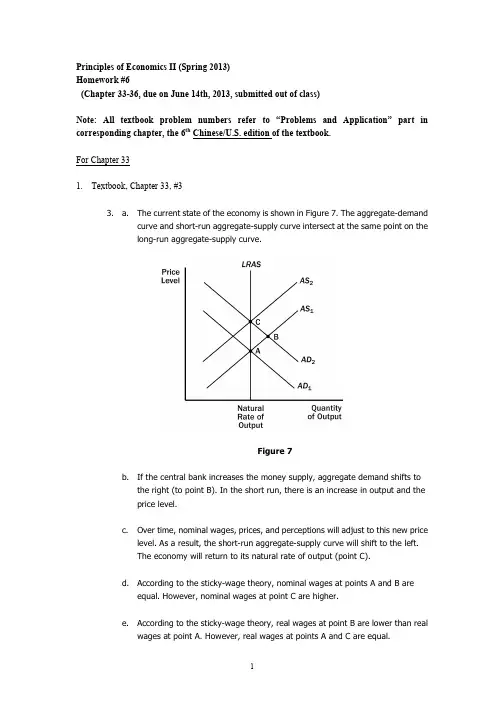
Principles of Economics II (Spring 2013)Homework #6(Chapter 33-36, due on June 14th, 2013, submitted out of class)Note: All textbook problem numbers refer to “Problems and Application” part in corresponding chapter, the 6th Chinese/U.S. edition of the textbook.For Chapter 331.Textbook, Chapter 33, #33. a. The current state of the economy is shown in Figure 7. The aggregate-demandcurve and short-run aggregate-supply curve intersect at the same point on thelong-run aggregate-supply curve.Figure 7b. If the central bank increases the money supply, aggregate demand shifts tothe right (to point B). In the short run, there is an increase in output and theprice level.c. Over time, nominal wages, prices, and perceptions will adjust to this new pricelevel. As a result, the short-run aggregate-supply curve will shift to the left.The economy will return to its natural rate of output (point C).d. According to the sticky-wage theory, nominal wages at points A and B areequal. However, nominal wages at point C are higher.e. According to the sticky-wage theory, real wages at point B are lower than realwages at point A. However, real wages at points A and C are equal.f. Yes, this analysis is consistent with long-run monetary neutrality. In the longrun, an increase in the money supply causes an increase in the nominal wage,but leaves the real wage unchanged.2.Textbook, Chapter 33, # 55. a. The statement that "the aggregate-demand curve slopes downward because itis the horizontal sum of the demand curves for individual goods" is false. Theaggregate-demand curve slopes downward because a fall in the price levelraises the overall quantity of goods and services demanded through the wealtheffect, the interest-rate effect, and the exchange-rate effect.b. The statement that "the long-run aggregate-supply curve is vertical becauseeconomic forces do not affect long-run aggregate supply" is false. Economicforces of various kinds (such as population and productivity) do affect long-runaggregate supply. The long-run aggregate-supply curve is vertical because theprice level does not affect long-run aggregate supply.c. The statement that "if firms adjusted their prices every day, then the short-runaggregate-supply curve would be horizontal" is false. If firms adjusted pricesquickly and if sticky prices were the only possible cause for the upward slope ofthe short-run aggregate-supply curve, then the short-run aggregate-supplycurve would be vertical, not horizontal. The short-run aggregate supply curvewould be horizontal only if prices were completely fixed.d. The statement that "whenever the economy enters a recession, its long-runaggregate-supply curve shifts to the left" is false. An economy could enter arecession if either the aggregate-demand curve or the short-runaggregate-supply curve shifts to the left.3.Textbook, Chapter 33, # 88. a. People will likely expect that the new chairman will not actively fight inflationso they will expect the price level to rise.b. If people believe that the price level will be higher over the next year, workerswill want higher nominal wages.c. At any given price level, higher labor costs lead to reduced profitability.d. The short-run aggregate-supply curve will shift to the left as shown in Figure10.Figure 10e. A decline in short-run aggregate supply leads to reduced output and a higherprice level.f. No, this choice was probably not wise. The end result is stagflation, whichprovides limited choices in terms of policies to remedy the situation.Figure 114.Textbook, Chapter 33, # 99. a. If households decide to save a larger share of their income, they must spendless on consumer goods, so the aggregate-demand curve shifts to the left, as shown in Figure 11. The equilibrium changes from point A to point B, so theprice level declines and output declines.b. If Florida orange groves suffer a prolonged period of below-freezingtemperatures, the orange harvest will be reduced. This decline in the naturalrate of output is represented in Figure 12 by a shift to the left in both theshort-run and long-run aggregate-supply curves. The equilibrium changesfrom point A to point B, so the price level rises and output declines.Figure 12Figure 13c. If increased job opportunities cause people to leave the country, the long-runand short-run aggregate-supply curves will shift to the left because there arefewer people producing output. The aggregate-demand curve will also shift tothe left because there are fewer people consuming goods and services. Theresult is a decline in the quantity of output, as Figure 13 shows. Whether theprice level rises or declines depends on the relative sizes of the shifts in theaggregate-demand curve and the aggregate-supply curves.5.Textbook, Chapter 33, #1111. a. If firms become optimistic about future business conditions and increaseinvestment, the result is shown in Figure 18. The economy begins at point Awith aggregate-demand curve AD1 and short-run aggregate-supply curve AS1.The equilibrium has price level P1 and output level Y1. Increased optimismleads to greater investment, so the aggregate-demand curve shifts to AD2.Now the economy is at point B, with price level P2 and output level Y2. Theaggregate quantity of output supplied rises because the price level has risenand people have misperceptions about the price level, wages are sticky, orprices are sticky, all of which cause output supplied to increase.Figure 18b. Over time, as the misperceptions of the price level disappear, wages adjust, orprices adjust, the short-run aggregate-supply curve shifts up to AS2 and theeconomy gets to equilibrium at point C, with price level P3 and output level Y1.The quantity of output demanded declines as the price level rises.c. The investment boom might increase the long-run aggregate-supply curvebecause higher investment today means a larger capital stock in the future,thus higher productivity and output.6.Textbook, Chapter 33, # 1212. Economy B would have a more steeply sloped short-run aggregate-supply curvethan would Economy A, because only half of the wages in Economy B are “sticky.”A 5% increase in the money supply would have a larger effect on output inEconomy A and a larger effect on the price level in Economy B.7.True or false? Keynes's primary message in The General Theory was that short-run economicfluctuations were the result of inadequate aggregate demand that could be corrected by using government policy.TrueFor Chapter 348.Textbook, Chapter 34, # 11. a. When the Fed’s bond traders buy bonds in open-market operations, themoney-supply curve shifts to the right from MS1 to MS2, as shown in Figure 1.The result is a decline in the interest rate.Figure 1 Figure 2b. When an increase in credit card availability reduces the cash people hold, themoney-demand curve shifts to the left from MD1 to MD2, as shown in Figure 2.The result is a decline in the interest rate.c. When the Federal Reserve reduces reserve requirements, the money supplyincreases, so the money-supply curve shifts to the right from MS1 to MS2, asshown in Figure 1. The result is a decline in the interest rate.d. When households decide to hold more money to use for holiday shopping, themoney-demand curve shifts to the right from MD1 to MD2, as shown in Figure3. The result is a rise in the interest rate.Figure 3e. When a wave of optimism boosts business investment and expands aggregatedemand, money demand increases from MD1 to MD2 in Figure 3. The increasein money demand increases the interest rate.Figure 49.Textbook, Chapter 34, # 22. a. The increase in the money supply will cause the equilibrium interest rate todecline, as shown in Figure 4. Households will increase spending and willinvest in more new housing. Firms too will increase investment spending. Thiswill cause the aggregate demand curve to shift to the right as shown in Figure5.Figure 5b. As shown in Figure 5, the increase in aggregate demand will cause an increasein both output and the price level in the short run (point B).c. When the economy makes the transition from its short-run equilibrium to itslong-run equilibrium, short-run aggregate supply will decline, causing the pricelevel to rise even further (point C).d. The increase in the price level will cause an increase in the demand for money,raising the equilibrium interest rate.e. Yes. While output initially rises because of the increase in aggregate demand,it will fall once short-run aggregate supply declines. Thus, there is no long-runeffect of the increase in the money supply on real output.10.Textbook, Chapter 34, # 3Figure 63. a. When fewer ATMs are available, money demand is increased and themoney-demand curve shifts to the right from MD1 to MD2, as shown in Figure6. If the Fed does not change the money supply, which is at MS1, the interestrate will rise from r1 to r2. The increase in the interest rate shifts theaggregate-demand curve to the left, as consumption and investment fall.b. If the Fed wants to stabilize aggregate demand, it should increase the moneysupply to MS2, so the interest rate will remain at r1 and aggregate demand willnot change.c. To increase the money supply using open market operations, the Fed shouldbuy government bonds.11.Textbook, Chapter 34, #88. a. The initial effect of the tax reduction of $20 billion is to increase aggregatedemand by $20 billion × 3/4 (the MPC) = $15 billion.b. Additional effects follow this initial effect as the added incomes are spent. Thesecond round leads to increased consumption spending of $15 billion × 3/4 =$11.25 billion. The third round gives an increase in consumption of $11.25billion × 3/4 = $8.44 billion. The effects continue indefinitely. Adding them allup gives a total effect that depends on the multiplier. With an MPC of 3/4, themultiplier is 1/(1 – 3/4) = 4. So the total effect is $15 billion × 4 = $60 billion.c. Government purchases have an initial effect of the full $20 billion, becausethey increase aggregate demand directly by that amount. The total effect of anincrease in government purchases is thus $20 billion × 4 = $80 billion. Sogovernment purchases lead to a bigger effect on output than a tax cut does.The difference arises because government purchases affect aggregatedemand by the full amount, but a tax cut is partly saved by consumers, andtherefore does not lead to as much of an increase in aggregate demand.d. The government could increase taxes by the same amount it increases itspurchases.12.Textbook, Chapter 34, # 99. If the marginal propensity to consume is 0.8, the spending multiplier will be 1/(1 – 0.8) = 5. Therefore, the government would have to increase spending by $400/5 = $80 billion to close the recessionary gap.13.Textbook, Chapter 34, 1111. a. Expansionary fiscal policy is more likely to lead to a short-run increase ininvestment if the investment accelerator is large. A large investmentaccelerator means that the increase in output caused by expansionary fiscalpolicy will induce a large increase in investment. Without a large accelerator,investment might decline because the increase in aggregate demand will raisethe interest rate.b. Expansionary fiscal policy is more likely to lead to a short-run increase ininvestment if the interest sensitivity of investment is small. Because fiscalpolicy increases aggregate demand, thus increasing money demand and theinterest rate, the greater the sensitivity of investment to the interest rate thegreater the decline in investment will be, which will offset the positiveaccelerator effect.For Chapter 3514.Textbook, Chapter 35, #11. Figure 8 shows two different short-run Phillips curves depicting these four points.Points A and D are on SRPC1 because both have expected inflation of 3%. Points Band C are on SRPC2 because both have expected inflation of 5%.Figure 815.Textbook, Chapter 35, #4Figure 144. a. Figure 14 shows the economy in long-run equilibrium at point A, which is onboth the long-run and short-run Phillips curves.b. A wave of business pessimism reduces aggregate demand, moving theeconomy to point B in the figure. The unemployment rate rises and theinflation rate declines. If the Fed undertakes expansionary monetary policy, itcan increase aggregate demand, offsetting the pessimism and returning theeconomy to point A, with the initial inflation rate and unemployment rate.c. Figure 15 shows the effects on the economy if the price of imported oil rises.The higher price of imported oil shifts the short-run Phillips curve up fromSRPC1 to SRPC2. The economy moves from point A to point C, with a higherinflation rate and higher unemployment rate. If the Fed engages inexpansionary monetary policy, it can return the economy to its originalunemployment rate at point D, but the inflation rate will be higher. If the Fedengages in contractionary monetary policy, it can return the economy to itsoriginal inflation rate at point E, but the unemployment rate will be higher. Thissituation differs from that in part (b) because in part (b) the economy stayedon the same short-run Phillips curve, but in part (c) the economy moved to ahigher short-run Phillips curve, which gives policymakers a less favorabletrade-off between inflation and unemployment.Figure 1516.Textbook, Chapter 35, #6Figure 166. If the Fed acts on its belief that the natural rate of unemployment is 4%, when thenatural rate is in fact 5%, the result will be a spiraling up of the inflation rate, asshown in Figure 16. Starting from a point on the long-run Phillips curve, with anunemployment rate of 5%, the Fed will believe that the economy is in a recession,because the unemployment rate is greater than its estimate of the natural rate.Therefore, the Fed will increase the money supply, moving the economy along theshort-run Phillips curve SRPC1. The inflation rate will rise and the unemploymentrate will fall to 4%. As the inflation rate rises over time, expectations of inflationwill rise, and the short-run Phillips curve will shift up to SRPC2. This process willcontinue, and the inflation rate will spiral upwards.The Fed may eventually realize that its estimate of the natural rate ofunemployment is wrong by examining the rising trend in the inflation rate.17.Textbook, Chapter 35, #77. a. If wage contracts have short durations, a recession induced by contractionarymonetary policy will be less severe, because wage contracts can be adjustedmore rapidly to reflect the lower inflation rate. This will allow a more rapidmovement of the short-run aggregate-supply curve and short-run Phillipscurve to restore the economy to long-run equilibrium.b. If there is little confidence in the Fed's determination to reduce inflation, arecession induced by contractionary monetary policy will be more severe. Itwill take longer for people's inflation expectations to adjust downwards.c. If expectations of inflation adjust quickly to actual inflation, a recessioninduced by contractionary monetary policy will be less severe. In this case,people's expectations adjust quickly, so the short-run Phillips curve shiftsquickly to restore the economy to long-run equilibrium at the natural rate ofunemployment.18.Textbook, Chapter 35, #9Figure 179. a. As shown in the left diagram of Figure 17, equilibrium output and employmentwill fall. However, the effects on the price level and inflation rate will beambiguous. The fall in aggregate demand puts downward pressure on prices,while the decline in short-run aggregate supply pushes prices up. The diagramon the right side of Figure 17 assumes that the inflation rate rises.b. The Fed would have to use expansionary monetary policy to keep output andemployment at their natural rates. Aggregate demand would have to shift toAD3.c. The Fed may not want to pursue this action because it will lead to a rise in theinflation rate as shown by point C.19.选举周期与经济波动:一个经济某一年的菲利普斯曲线由下列的关系式确定:π = πe - (u - 4%)。

曼昆《宏观经济学》(第6、7版)第13章总供应与通货膨胀和失业之间旳短期权衡复习笔记跨考网独家整顿最全经济学考研真题,经济学考研课后习题解析资料库,您可以在这里查阅历年经济学考研真题,经济学考研课后习题,经济学考研参照书等内容,更有跨考考研历年辅导旳经济学学哥学姐旳经济学考研经验,从前辈中获得旳经验对初学者来说是宝贵旳财富,这或许能帮你少走弯路,躲开某些陷阱。
如下内容为跨考网独家整顿,如您还需更多考研资料,可选择经济学一对一在线征询进行征询。
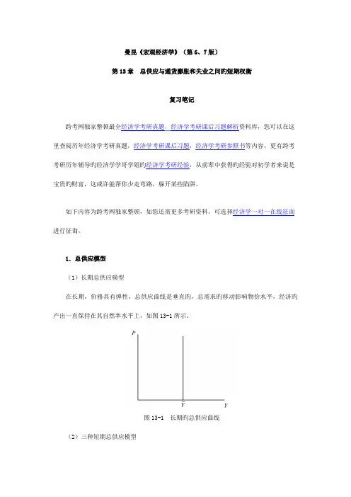
1.总供应模型(1)长期总供应模型在长期,价格具有弹性,总供应曲线是垂直旳,总需求旳移动影响物价水平,经济旳产出一直保持在其自然率水平上,如图13-1所示。
图13-1 长期旳总供应曲线(2)三种短期总供应模型三种短期总供应模型都认为市场旳某种不完善性使经济旳产出背离其自然率水平,成果短期总供应曲线向右上方倾斜,而不是垂直旳,总需求曲线旳移动引起产出水平临时背离其自然率。
得出了相似旳短期总供应方程式:(),0e Y Y P P αα=+->其中,Y 为产出,Y 为自然产出,P 为物价水平,e P 为预期旳物价水平,参数α表达产出对未预期到旳物价水平变动旳反应程度,1/α是总供应曲线旳斜率。
这个方程式阐明,当物价水平背离预期旳物价水平时,产出背离其自然率水平。
①黏性工资模型在黏性工资模型中,在短期内假设劳动市场失灵,名义工资具有黏性,不能随劳动旳供求状况立即调整。
未预期到旳物价水平上涨不会立即影响名义工资,则实际工资(/W P )下降,更低旳实际工资使企业雇佣更多劳动力,从而导致产出增长。
如图13-2所示,图(a )表达劳动需求曲线。
由于名义工资W 是黏住不变旳,当物价水平从1P 上升届时2P ,实际工资从(1W P /)下降到(2/W P ),较低旳实际工资使劳动需求量从1L上升到2L 。
图(b )表达生产函数,当劳动量从1L 上升届时2L ,产出从1Y 增长到2Y 。