Numerical Simulation of Azimuthal Uniformity of Injection Currents in Single-Point-Feed I
- 格式:pdf
- 大小:971.55 KB
- 文档页数:6

第28卷㊀第2期2024年2月㊀电㊀机㊀与㊀控㊀制㊀学㊀报Electri c ㊀Machines ㊀and ㊀Control㊀Vol.28No.2Feb.2024㊀㊀㊀㊀㊀㊀基于非线性建模与拟合的永磁同步电机转子初始位置精确估计方法姚培煜1,㊀冯国栋1,㊀吴轩2,㊀彭卫文1,㊀丁北辰3(1.中山大学智能工程学院,广东深圳518107;2.湖南大学电气与信息工程学院,湖南长沙410082;3.中山大学先进制造学院,广东深圳518107)摘㊀要:针对永磁同步电机转子初始位置估计的精度与收敛速度受限问题,提出一种基于高频信号注入的非线性建模与拟合实现的初始位置估计方法㊂首先,建立初始位置与高频信号响应的关联模型,表明高频响应可用于直接计算初始位置,但直接计算结果在大部分转子位置易受测量噪声的影响㊂为此,提出基于多项式模型建立位置估计非线性模型,选取合适的模型参数,利用少量测试点拟合该模型,即可实现初始位置的快速精确估计,有效提高了估计精度与系统抗干扰能力㊂实验与仿真结果表明,相比现有方法,提出的方法易于实现,无需复杂滤波器与观测器设计,仅需要选取少量测试点即可快速估计精确转子初始位置,在保证估计精度的同时改进了传统估计方法收敛速度慢问题㊂关键词:永磁同步电机;高频信号注入;转子初始位置估计;多项式模型;非线性模型DOI :10.15938/j.emc.2024.02.014中图分类号:TM351文献标志码:A文章编号:1007-449X(2024)02-0142-10㊀㊀㊀㊀㊀㊀㊀㊀㊀㊀㊀㊀㊀㊀㊀㊀㊀㊀㊀㊀㊀㊀㊀㊀㊀㊀㊀㊀㊀㊀㊀㊀㊀㊀㊀㊀㊀㊀㊀㊀㊀㊀㊀㊀㊀㊀㊀㊀㊀㊀㊀㊀㊀㊀㊀㊀㊀㊀㊀㊀㊀㊀㊀㊀㊀㊀㊀㊀㊀㊀㊀㊀㊀㊀㊀㊀㊀㊀㊀㊀㊀㊀㊀㊀㊀㊀㊀㊀㊀㊀㊀㊀㊀㊀㊀㊀㊀㊀㊀㊀㊀㊀㊀㊀㊀㊀㊀㊀㊀㊀㊀㊀㊀㊀收稿日期:2022-09-24基金项目:国家自然科学基金(52105079,62103455)作者简介:姚培煜(1999 ),男,硕士研究生,研究方向为永磁同步电机无位置传感控制;冯国栋(1988 ),男,博士,副教授,硕士生导师,研究方向为新能源汽车电机系统控制关键技术;吴㊀轩(1983 ),男,博士,副教授,研究方向为电力电子与电力传动㊁大型风力发电技术㊁特种车辆电驱动技术;彭卫文(1987 ),男,博士,副教授,研究方向为系统可靠性㊁智能系统的状态监测㊁故障预测与健康管理;丁北辰(1990 ),男,博士,副教授,研究方向为机器人控制与新能源汽车动力系统控制㊂通信作者:丁北辰High precision initial rotor position estimation method for permanent magnet synchronous motor based on nonlinear modeling and fittingYAO Peiyu 1,㊀FENG Guodong 1,㊀WU Xuan 2,㊀PENG Weiwen 1,㊀DING Beichen 3(1.School of Intelligent Systems Engineering,Sun Yat-sen University,Shenzhen 518107,China;2.College of Electrical and Information Engineering,Hunan University,Changsha 410082,China;3.School of Advanced Manufacturing,Sun Yat-sen University,Shenzhen 518107,China)Abstract :Aiming at the problem that the accuracy and convergence speed of rotor initial position estima-tion of permanent magnet synchronous motor are limited,a nonlinear modeling and fitting method basedon high-frequency signal injection was proposed.Firstly,the correlation model between the initial posi-tion and the high-frequency signal response was established,which shows that the high-frequency re-sponse can be used to calculate the initial position directly,but the direct calculation results are vulnera-ble to the measurement noise in most rotor positions.To solve this issue,a polynomial model was used toestablish the nonlinear model of location estimation,suitable model parameters were selected and a few oftest points were used to fit the polynomial model to achieve rapid and accurate calculation of the initialposition,which effectively improves the estimation accuracy and anti-interference ability of the system. The experimental and simulation results show that compared with the existing methods,in the proposed method it is easy to implement,complex filter and observer design is not needed,and only a few test points need to be selected to quickly estimate the initial position of the precise rotor,which ensures the estimation accuracy and improves the problem of slow convergence of the traditional estimation methods. Keywords:permanent magnet synchronous motor;high frequency signal injection;initial rotor position es-timation;polynomial model;nonlinear model0㊀引㊀言永磁同步电机(permanent magnet synchronous motor,PMSM)因其结构简单,高效率,高能量密度等优点而被广泛应用于新能源汽车等多个领域[1-3]㊂对于永磁同步电机伺服系统,转子初始位置是保证电机启动性能的重要参数㊂具体而言,精确的初始位置能够提高电机控制性能,若初始位置误差过大,会降低启动性能,甚至会导致电机反转与启动失败[4-6]㊂转子位置可通过光电编码器,旋转变压器等获取,但增加了系统成本和体积,在低成本应用如家用电器以及超高速电机应用中,无位置传感控制技术被广泛应用㊂初始位置估计是无位置传感控制的重要环节,可有效地提高系统启动与控制的可靠性㊂因此,转子初始位置估计对永磁同步电机伺服系统十分关键㊂转子初始位置估计在文献中已有广泛研究㊂其中,利用电感饱和效应是近年来解决转子初始位置估计的重要手段,可分为脉冲电压法[7-10],高频信号注入法[11-23]㊂脉冲电压法通过注入一系列脉冲电压矢量,利用电流响应估计转子位置㊂然而,脉冲电压注入可导致转子转动,且过程耗时长㊂高频信号注入法实现简单,无需电机参数和额外硬件,可分高频旋转电压注入[11-16]和高频脉振电压注入[17-23]㊂高频旋转电压注入法依赖于转子凸极效应,且需要通过坐标变换和滤波器提取转子位置㊂文献[11]对高频电流响应进行低通滤波,根据电流幅值随转子位置变化实现转子位置估计㊂文献[14]对三相高频电流正㊁负序分量分离,利用任意一相正负序相角差估计转子位置㊂文献[15]分析了旋转高频注入方法受采样㊁滤波器的影响,并提出一种补偿算法提高位置观测精度㊂高频脉振电压注入法对凸极性要求不高,适用于表贴式电机㊂文献[17]针对相移问题,改用交直轴响应电流解调去除高频分量㊂文献[18]通过对虚拟直轴施加高频电压产生一系列振动信号实现初始位置估计㊂但该方法需要振动传感器,且在转动惯量较大的应用中,需要较大电流诱导转子振动㊂文献[20]在脉振注入基础上引入载波频率成分法判断磁极极性,避免二次信号注入,简化了实现步骤㊂现有高频信号注入估计方法大多通过滤波环节分离高频信号,再通过观测器估计转子初始位置㊂但滤波器对高频信号的幅值和相位产生影响,限制了系统带宽,无法同时保证转子位置的辨识精度和辨识速度㊂同时,观测器的设计也依赖高频信号响应和电机参数㊂针对以上问题,本文提出一种基于高频信号注入的非线性建模与拟合方法,实现转子初始位置估计㊂在虚拟直轴注入高频信号,解调高频电流响应即可获得初始位置,但易受转子所在位置的影响㊂在此基础上,提出基于非线性建模的初始位置估计方法,利用少数测试对非线性模型辨识,实现对转子位置的精确估计㊂此方法无需复杂滤波器和观测器设计,避免相位偏移和收敛速度慢等问题㊂此外,采用测试点快速拟合估计模型有效提高初始位置估计精度和收敛速度㊂仿真与实验结果验证提出方法的有效性㊂1㊀高频信号注入建模永磁同步电机d-q轴电压方程可表示为:u d=Ri d+L dd i dd t-ωL q i q;u q=Ri q+L qd i qd t+ωL d i d+ωλ0㊂üþýïïïï(1)式中:u d/q㊁i d/q和L d/q分别表示d-q轴电压㊁电流和电感;λ0是永磁磁链;R是绕组电阻;ω是电角速度㊂对应的高频信号注入模型可表示为:u dh=R h i dh+L dhd i dhd t;u qh=R h i qh+L qhd i qhd t㊂üþýïïïï(2)341第2期姚培煜等:基于非线性建模与拟合的永磁同步电机转子初始位置精确估计方法式中下标h 表示高频分量㊂例如L dh /qh 表示高频电感,R h 表示高频电阻,初始转速为0㊂不失一般性,假设电机转子的初始位置为θ0㊂定义一个虚拟d -q 轴,其虚拟d 轴的位置为θv ,而θ0和θv 间的误差定义为Δθ=θv -θ0,虚拟d -q 轴与真实d -q 轴的关系如图1所示㊂图1㊀虚拟d -q 轴与真实d -q 轴的关系Fig.1㊀Relationship between virtual and actualdq-axis为估计初始位置θ0,将高频电压信号注入虚拟d 轴,可表达为u dh,v =V dh cos(ωh t )㊂(3)式中:u dh,v 表示高频电压;V dh 为幅值;ωh 为频率㊂基于旋转变换可得注入实际d 轴的高频电压信号为:u dh =u dh,v cosΔθ;u qh =u dh,vsinΔθ㊂}(4)式中u dh 和u qh 为注入到真实d -q 轴的高频电压㊂将式(3)和式(4)代入式(2)可得d -q 与α-β轴下的高频电流响应为:㊀i dh =I dd sin(ωh t -φd )cosΔθ;i qh=I dqsin(ωht -φq)sinΔθ㊂}(5)㊀i αh =I dd sin(ωh t +φd )cosΔθcos θ0-I dq sin(ωh t +φq )sinΔθsin θ0;i βh =I dd sin(ωh t +φd )cosΔθsin θ0+I dqsin(ωht +φq)sinΔθcos θ0㊂üþýïïïï(6)㊀I dd =V dh Z dh ;I dq =V dh Z qh;Z 2dh =R 2h +ω2h L 2dh ;Z 2qh =R 2h +ω2h L 2qh ;tan φd =R h ωh L dh ;tan φq =R h ωh L qh㊂üþýïïïïïï(7)式中i αh 和i βh 可由abc 相电流计算获取㊂对α-β轴高频电流进行如下运算,即:M αs ≜avg(i αh sin ωh t )=I 1cosΔθcos θ0-I 2sinΔθsin θ0;M βs≜avg(i βhsin ωht )=I 1cosΔθsin θ0+I 2sinΔθcos θ0㊂}(8)式中: avg(x ) 表示x 在一个或多个周期内的平均值(例如信号x 的5个周期),I 1和I 2表示如下:I 1=0.5I dd cos φd ;I 2=0.5I dq cos φq ㊂}(9)2㊀转子初始位置直接计算2.1㊀高频注入直接计算法原理式(8)存在3个未知数,至少需要两组数据确定θ0㊂为此,将高频信号分别注入2个虚拟d 轴,对应位置分别为θv0和θv1,其中:1)将V dh0cos(ωh0)注入虚拟d 轴θv0,得到i αh0和i βh0;2)将V dh1cos(ωh1)注入虚拟d 轴θv1,得到i αh1和i βh1㊂基于式(8)以及i αh i 和i βh i ,i =0㊁1,可得:M αs0=I 1cos(θv0-θ0)cos θ0-I 2sin(θv0-θ0)sin θ0;M βs0=I 1cos(θv0-θ0)sin θ0+I 2sin(θv0-θ0)cos θ0;M αs1=I 1cos(θv1-θ0)cos θ0-I 2sin(θv1-θ0)sin θ0;M βs1=I 1cos(θv1-θ0)sin θ0+I 2sin(θv1-θ0)cos θ0㊂üþýïïïï(10)不难看出,基于式(10)可直接计算转子初始位置,定义计算出的位置为θr ㊂特别地,当选择虚拟位置满足θv0=0和θv1=π/2时,θr 可表示为:2θr =arccos(cos2θ0),sin2θ0ȡ0;2π-arccos(cos2θ0),sin2θ<0㊂{(11)其中:sin2θ0=B2C -A 2;cos2θ0=DA 2C -A 2㊂üþýïïïï(12)A =M αs0+M βs1=I 1+I 2;B =2M αs1=(I 1-I 2)sin2θ0;C =M 2αs0+M 2βs1+2M 2αs1=I 21+I 22;D =M 2αs0-M 2βs1=(I 21-I 22)cos2θ0㊂üþýïïïïï(13)图2给出了直接计算法的实施流程,高频信号依次注入得到α-β轴高频电流响应,通过式(10)~式(13)计算出转子初始位置的估计值θr ,最后使用短脉冲注入方法辨识转子磁极极性[24]㊂2.2㊀直接计算法估计误差分析不难看出直接计算法的估计误差与高频信号注入的虚拟位置θv0与θv1相关㊂定义直接计算法的估计误差为Δθe =θr -θ0㊂本节研究θv0与θv1的选择与441电㊀机㊀与㊀控㊀制㊀学㊀报㊀㊀㊀㊀㊀㊀㊀㊀㊀㊀㊀㊀㊀第28卷㊀估计误差Δθe 的关系,指导θv0与θv1的选择㊂图2㊀直接计算法框图Fig.2㊀Block diagram of direct calculation method2.2.1㊀虚拟位置θv0和θv1选择与误差Δθe 的关系直接计算法是将式(3)中的高频信号分别注入虚拟位置θv0和θv1,获得α-β轴高频响应,对其进一步处理得方程组(10),包含3个未知量,利用数值计算可获得估计结果㊂图3为分别在2个转子初始位置θ0下选择任意不同θv0和θv1时,直接计算法估计误差的分布图,图中每个误差点都是在噪声强度为30dB 仿真环境下2000次随机试验的平均值㊂下文若无特别说明,仿真环境中的噪声强度统一为30dB㊂不难看出,当θv0和θv1越接近,Δθe 越大;当θv0=θv1时,式(10)中的方程式个数变为2个,方程组无解;当θv0和θv1的差值越大,估计误差受噪声影响越小㊂θv0和θv1分别取0和π/2时估计误差相对最小㊂图3㊀不同θv0和θv1的估计误差分布Fig.3㊀Estimation error distributions of different θv0and θv12.2.2㊀不同转子位置的误差Δθe 分析本节探讨转子在不同初始位置直接计算法的估计误差㊂图4给出了不同转子位置的估计误差㊂其中,虚拟位置设置为θv0=0和θv1=π/2;每个误差点都是对同一位置2000次随机试验的平均值㊂可以看出θ0在[0,π]上的估计误差Δθe 呈现三角函数规律变化,在θ0=0㊁π/2㊁π/4附近时θr 的误差Δθe 较小,最小误差约为0.01rad,而在θ0=π/4㊁3π/4附近时θ0的误差Δθe 非常大,最大误差为0.063rad,最大误差是最小误差的6倍以上㊂导致误差呈三角函数规律变化的原因如下:在式(10)中噪声来源于M αs 和M βs ,而在使用式(10)求解θr 时,对cos2θ0进行反三角变化求解θr ㊂对式(10)等式右边变换拆解,提取含有cos2θ0的部分为:S αs =0.5(cos θv (I 1-I 2)cos2θ0)M αs ;S βs =0.5(sin θv (I 1-I 2)cos2θ0)M βs㊂üþýïïïï(14)式中:S αs 和S βs 可以近似表示信号与噪声的比例,即信噪比(signal to noise ratio,SNR)㊂当θ0接近π/4㊁3π/4时,cos2θ0趋于0,S αs 和S βs 趋于0㊂θ0趋于0㊁π/2㊁π时,cos2θ0趋于1,S αs 和S βs 远大于0㊂即Δθe 随着cos2θ0变化而波动㊂不难发现,由于测量噪声的存在,基于式(10)的直接计算法的估计误差在不同转子位置的波动非常大,特别是转子位置在π/4㊁3π/4附近的估计误差比最小误差增加了6倍㊂因此,本文提出基于非线性建模与拟合的方法估计初始位置,提高估计精度和降低估计误差的波动㊂图4㊀直接计算法在不同转子位置的误差变化Fig.4㊀Error variation of direct calculation method atdifferent rotor positions3㊀基于非线性建模与拟合的初始转子位置估计3.1㊀基于多项式建模与曲线拟合的估计方法基于式(8),定义M s ≜M 2αs +M 2βs =I 22+(I 21-I 22)cos 2(θv -θ0)㊂(15)541第2期姚培煜等:基于非线性建模与拟合的永磁同步电机转子初始位置精确估计方法式中M s 以虚拟d 轴位置θv 为自变量的函数,且M s在θv 满足下式时取最大值:Δθ=θv -θ0=0or π㊂(16)如图5所示,考虑在一个周期内,函数M s (θv )在θv <θ0时递增,在此处后递减,这表明转子初始位置θ0可在函数曲线M s (θv )的最大值处得到㊂图5㊀θ0=π/2时M s (θv )曲线Fig.5㊀Curve of M s (θv )at θ0=π/2考虑到直接计算法受测量噪声影响较大,本文提出利用多项式函数对M s (θv )建模,进而在M s (θv )的最大值处确定初始位置θ0㊂不失一般性,本文使用k 阶多项式对M s (θv )建模,即M s (θv )=a k θk v +a k -1θk -1v+ +a 1θv +a 0㊂(17)式中a 0, ,a k -1,a k 为k 阶多项式的系数,可通过曲线拟合估计㊂当a 0, ,a k -1,a k 确定,初始位置θ0可以通过求解下式获得:d M s (θv )d θv =ka k θk -1v +(k -1)a k -1θk -2v+ +2a 2θv +a 1=0㊂(18)当k =2或3时,θ0的估计为:θ0=-a 12a 2,k =2;-a 2ʃa 22-3a 3a 13a 3ɪ[0,π2],k =3㊂ìîíïïïï(19)综上,基于提出的初始位置估计分为两步:第一步:设置N 个虚拟d 轴位置,注入高频测试信号并采集数据用于拟合M s (θv );第二步:基于最小二乘估计a 0, ,a k -1,a k ,并用式(19)计算初始位置θr ㊂图6给出了第一步的图解,假设N 个虚拟d 轴位置为{θv1,θv2, ,θv N },通过电流计算获得{M s1,M s2, ,M s N }㊂基于上述数据与最小二乘法拟合的多项式系数可表示为a =(ϕT ϕ)-1ϕT M ㊂(20)式中:a =[a 0,a 1, ,a k ]T ;ϕ=θk v1θk -1v1θv11θk v2θk -1v2 θv21︙︙︙︙θk v N θk -1v N θv N 1éëêêêêêêùûúúúúúú;M =[M s1,M s2, ,M s N ]T ㊂üþýïïïïïïïïï(21)图6㊀第一步的步骤图Fig.6㊀Diagram of the first step图7给出了此方法的实施框图㊂定义测试点固定间距为θL ,高频电压信号依次注入d 轴虚拟位置θv i =θv i -1+θL ,i =1, ,N ㊂采集α-β轴电流响应,利用式(15)计算M s (θv )用于建模与拟合,利用式(19)计算初始位置θ0㊂图7㊀拟合估计法框图Fig.7㊀Block diagram of fitting estimation method3.2㊀多项式模型参数选择首先,讨论如何选择合适的参数k ㊂一般选择k =2~4可满足估计精度要求㊂考虑到实际环境中的测量噪声,图8为使用不同阶次的多项式拟合M s (θv )㊂从表1不难发现,曲线拟合误差随着k 的增加而越小,但在θ0附近使用二阶多项式拟合即可实现较好的拟合精度㊂641电㊀机㊀与㊀控㊀制㊀学㊀报㊀㊀㊀㊀㊀㊀㊀㊀㊀㊀㊀㊀㊀第28卷㊀表1㊀不同阶次多项式的拟合精度比较Table 1㊀Comparison of fitting precision between differentorder polynomials参数转子位置/rad 拟合误差/rad真实位置θ00.7854 二阶多项式0.83080.0454三阶多项式0.82730.0419四阶多项式0.82560.0402图8㊀不同阶次多项式拟合M s (θv )Fig.8㊀Fitting M s (θv )with different order polynomials拟合k 次多项式最少需要k +1个拟合点,即N ȡk +1㊂其次,研究如何选取合适的虚拟位置{θv1,θv2, ,θv N },保证初始位置估计精度㊂图9给出了选择k =2㊁N =3㊁4㊁5时的估计误差㊂从图9中不难发现拟合点数量N =5较N =4拟合精度提升并不明显,但需要增加测试点;而N =4较于N =3估计精度有显著提高,且N =4对应的估计精度已满足应用需求㊂综合实现复杂度与估计精度要求,本文选择N =4个拟合点实现多项式模型的拟合㊂图9㊀不同拟合点数量的估计误差Fig.9㊀Estimation error between different number offitting points直接计算法估计的θr 可用于确定一个θ0的粗略分布区域㊂假定θ0=π/4㊁k =2㊁N =4㊂分别在区间R 1=[0,π/2]㊁R 2=[π/8,3π/8]和R 3=[3π/16,5π/16]内随机选取拟合点进行曲线拟合估计,表2是进行2000次随机实验的平均误差,表明通过θr 确定一个合适的区间可以有效地提高估计精度㊂表2㊀不同拟合点选取区间的拟合精度比较Table 2㊀Comparison of fitting precision between differentselection interval of fitting points参数转子位置/rad 拟合误差/rad 真实位置θ00.7854R 10.95280.1674R 20.95680.1714R 30.89680.1114M s (θv )曲线在峰值附近以峰值为中心左右对称,因此在两侧对称选取拟合点能有效提高拟合效果㊂考虑到估计的θr 接近峰值位置,因此本文选择在θr 左右对称地选取拟合点㊂具体而言,首先确定左侧第一个拟合点,其次在当前位置叠加θL 确定下一拟合点位置,该过程可表示为θ2=θ1+θL , ,θN =θN -1+θL ㊂(22)式中θL 对拟合结果有显著影响㊂假定θ0=π/4㊁k =2㊁N =4,图10给出了选择不同θL 时估计误差的变化曲线㊂不难看出,选择θL =0.558rad 估计误差最小㊂综上,本文选择二阶多项式四点拟合,其中拟合点以直接计算值θr 左右对称等间距θL =0.558rad 选取㊂图10㊀不同拟合点间距的估计误差Fig.10㊀Estimation error under different θL3.3㊀多项式曲线拟合法仿真实验本节通过仿真结果验证提出方法的有效性㊂上文分析得出k 阶多项式参数k =2㊁N =4以及拟合点741第2期姚培煜等:基于非线性建模与拟合的永磁同步电机转子初始位置精确估计方法间距选择θL =0.558rad,具有较高的估计精度,下文仿真实验都将使用此模型参数㊂图11是假定初始位置θ0=π/4时,分别使用直接计算法和拟合估计法进行2000次随机实验的估计误差分布㊂不难发现,相比于直接计算法,曲线拟合估计法在同一转子位置上的估计误差和误差波动都更小㊂图11㊀2000次随机实验的估计误差分布Fig.11㊀Estimated error distributions for 2000randomized tests图12为使用高频注入直接计算法和曲线拟合估计法在不同转子位置上的估计误差比较,图12(a)㊁(b)分别为30dB 和40dB 测量噪声下的结果㊂图中每点都是进行了2000次实验的平均估计误差㊂可以发现在θ0=π/4㊁3π/4附近的大部分区域,拟合误差远小于直接计算误差,差值最大的位置拟合误差较直接计算误差减小了0.0352rad,减小了56%㊂另外,对比不同噪声强度环境可以发现,曲线拟合估计法在不同噪声强度下都能够保持较大幅度的估计精度提升㊂曲线拟合法在超过80%的转子位置上估计误差小于直接计算法,在一些位置误差能减小50%以上㊂但在θ0=0㊁π/2㊁π附近其余20%的位置上,因信噪比较大,直接计算法估计误差小于曲线拟合法㊂因此在一个电角度周期内,可以采用两种方法混合估计,当θ0在0㊁π/2㊁π附近小部分区域时令θr 为最终估计结果,否则进一步实施拟合方法估计初始位置,如表3所示㊂图12㊀不同转子位置上估计误差对比Fig.12㊀Comparison of estimated errors between differ-ent rotor positions表3㊀不同转子位置上3种方法的区别Table 3㊀Difference of three methods between differentrotor positions方法θ0在0㊁π/2㊁π附近其他位置直接计算法直接计算直接计算拟合估计法拟合估计拟合估计混合估计法直接计算拟合估计在所有位置上,θr 的平均误差为0.0432rad,拟合θ0的平均误差为0.0268rad,混合估计法可使平均误差进一步减小到0.0248rad㊂整体估计精度提高40%,且拟合估计值的误差波动更小㊁更平稳㊂4㊀实验验证在图13所示的PMSM 样机实验平台上验证本文所提出的方法㊂实验电机的设计参数如表4所示㊂测试电机配备高分辨率光学编码器,单转脉冲数(PPR)为2500㊂从该编码器测量的转子位置将被用来评估提出估计方法的性能,不参与实际控制㊂在实验平台验证方法过程中,电机的转速与转矩都为0㊂注入高频信号的参数为:注入信号频率ωh =150Hz,注入信号幅值V dh =20V㊂选择的非线性模型参数为:k =2㊁N =4㊁θL =0.558rad㊂图14出了使用此参数对M s (θv )进行建模估计θ0的例子㊂841电㊀机㊀与㊀控㊀制㊀学㊀报㊀㊀㊀㊀㊀㊀㊀㊀㊀㊀㊀㊀㊀第28卷㊀图13㊀实验装置Fig.13㊀Experimental device 表4㊀实验电机的设计参数Table 4㊀Design parameters of experimental motor图14㊀实验验证的拟合估计法例子Fig.14㊀Examples of fitting estimation method verifiedby experiment首先,实验一在不同转子位置进行实验以评估提出估计方法的效果㊂图15(a)给出了电机一个电角度周期内8个位置的估计结果,不难发现估计结果与真实位置十分接近,具体误差分布见图15(b)㊂从图15可以看出,一个电角度周期内,最大拟合误差0.0412rad,最小拟合误差0.0035rad,平均拟合误差约为0.018rad㊂结果表明,曲线拟合估计法能精确估计转子初始位置㊂其次,实验二对比直接计算法与拟合估计法的实验结果㊂直接计算法从α-β轴高频响应电流计算转子初始位置,曲线拟合估计法采用二阶多项式四点非线性建模与拟合估计转子位置㊂估计结果对比如图16(a)所示,2种方法的估计误差对比如图16(b)所示㊂可以看出,直接计算法的平均估计误差为0.034rad,最大估计误差0.114rad,拟合估计的平均拟合误差为0.016rad,最大拟合误差0.042rad㊂实验证明提出的方法相比于传统高频注入法大幅提升了估计精度,降低了误差波动㊂图15㊀实验一的转子初始位置估计结果Fig.15㊀Rotor initial position estimation results inexperiment 1图16㊀实验二的转子初始位置估计结果比较Fig.16㊀Comparison of rotor initial position estimationresults in experiment 25㊀结㊀论本文提出一种基于高频注入的非线性建模与拟合的转子初始位置估计方法,并通过仿真和实验验941第2期姚培煜等:基于非线性建模与拟合的永磁同步电机转子初始位置精确估计方法证提出方法的有效性㊂提出的方法利用少数测试点对位置估计非线性模型快速拟合,实现简单,不依赖电机参数,无需复杂滤波器和观测器的设计㊂实验结果表明,最大误差小于0.05rad,平均误差小于0.02rad㊂与现有方法相比,提出的方法具有估计精度高,收敛速度快,易于实现等优势,工程实用价值高㊂此外,该方法同样在无位置传感器控制技术上有潜在的应用前景㊂参考文献:[1]㊀SHOU W,KANG J,DEGANO M,et al.An accurate wide-speedrange control method of IPMSM considering resistive voltage drop and magnetic saturation[J].IEEE Transactions on Industrial E-lectronics,2020,67(4):2630.[2]㊀朱元,肖明康,陆科,等.电动汽车永磁同步电机转子温度估计[J].电机与控制学报,2021,25(6):72.ZHU Yuan,XIAO Mingkang,LU Ke,et al.Rotor temperature estimation for permanent magnet synchronous motors in electric ve-hicles[J].Electric Machines and Control,2021,25(6):72. [3]㊀王晓远,刘铭鑫,陈学永,等.电动汽车用ANGN带滤波补偿三阶滑模自抗扰控制[J].电机与控制学报,2021,25(11):25.WANG Xiaoyuan,LIU Mingxin,CHENG Xueyong,et al.Third-order sliding mode active disturbance rejection control of PMSM with filter compensation for electric vehicle[J].Electric Machines and Control,2021,25(11):25.[4]㊀BRIZ F,DEGNER M.Rotor position estimation[J].IEEE Indus-trial Electronics Magazine,2011,5(2):24.[5]㊀YEH H,YANG S.Phase inductance and rotor position estimationfor sensorless permanent magnet synchronous machine drives at standstill[J].IEEE Access,2021(9):32897.[6]㊀贾洪平,贺益康.基于高频注入法的永磁同步电动机转子初始位置检测研究[J].中国电机工程学报,2007,27(15):15.JIA Hongping,HE Yikang.Study on inspection of the initial rotor position of a PMSM based on high-frequency signal injection[J].Proceedings of the CSEE,2007,27(15):15.[7]㊀张树林,康劲松,母思远.基于等宽电压脉冲注入的永磁同步电机转子初始位置检测方法[J].中国电机工程学报,2020,40(19):6085.ZHANG Shulin,KANG Jinsong,MU Siyuan.Initial rotor position detection for permanent magnet synchronous motor based on identi-cal width voltage pulse injection[J].Proceedings of the CSEE, 2020,40(19):6085.[8]㊀王宾,彭皆彩,于水娟.一种电流合成的PMSM转子初始位置检测方法[J].电机与控制学报,2020,24(8):67.WANGBin,PENG Jiecai,YU Shuijuan.Method to detect the ini-tial rotor position of PMSM based on current synthesis[J].Elec-tric Machines and Control,2020,24(8):67.[9]㊀孟高军,余海涛,黄磊,等.一种基于线电感变化特征的永磁同步电机转子初始位置检测新方法[J].电工技术学报, 2015,30(20):1.MENG Gaojun,YU Haitao,HUANG Lei,et al.A novel initial rotor position estimation method for PMSM based on variation be-havior of line inductances[J].Transactions of China Electrotech-nical Society,2015,30(20):1.[10]㊀WU X,LU Z,LING Z,et al.An improved pulse voltage injec-tion based initial rotor position estimation method for PMSM[J].IEEE Access,2021(9):121906.[11]㊀鲁家栋,刘景林,卫丽超.永磁同步电机转子初始位置检测方法[J].电工技术学报,2015,30(7):105.LU Jiadong,LIU Jinglin,WEI Lichao.Estimation of the initialrotor position for permanent magnet synchronous motors[J].Transactions of China Electrotechnical Society,2015,30(7):105.[12]㊀JIN X,NI R,CHEN W,et al.High-frequency voltage-injectionmethods and observer design for initial position detection of per-manent magnet synchronous machines[J].IEEE Transactions onPower Electronics,2018,33(9):7971.[13]㊀王华斌,施金良,陈国荣,等.内嵌式永磁同步电机转子初始位置检测[J].电机与控制学报,2011,15(3):40.WANG Huabin,SHI Jinliang,CHEN Guorong,et al.Initial ro-tor position detection of IPMSM[J].Electric Machines and Con-trol,2011,15(3):40.[14]㊀刘景林,鲁家栋.基于相电流正负序分量相角差的高精度内置式永磁同步电机转子初始位置检测方法[J].电工技术学报,2016,31(23):63.LIU Jinglin,LU Jiadong.High-precision estimation method of in-itial rotor position for IPMSM based on phase difference of posi-tive and negative sequence current component[J].Transactionsof China Electrotechnical Society,2016,31(23):63. [15]㊀杨健,杨淑英,李浩源,等.基于旋转高频电压注入的永磁同步电机转子初始位置辨识方法[J].电工技术学报,2018,33(15):3547.YANG Jian,YANG Shuying,LI Haoyuan,et al.Initial rotor po-sition estimation for IPMSM based on high frequency rotating volt-age injection[J].Transactions of China Electrotechnical Society,2018,33(15):3547.[16]㊀SHUANG B,ZHU Z.A novel sensorless initial position estima-tion and startup method[J].IEEE Transactions on Industrial E-lectronics,2021,68(4):2964.[17]㊀于安博,刘利,阚志忠,等.高频脉振信号注入永磁同步电机无滤波器初始位置辨识方法[J].电工技术学报,2021,36(4):801.YU Anbo,LIU Li,KAN Zhizhong,et al.Initial position identi-051电㊀机㊀与㊀控㊀制㊀学㊀报㊀㊀㊀㊀㊀㊀㊀㊀㊀㊀㊀㊀㊀第28卷㊀fication of PMSM with filterless high frequency pulse signal injec-tion method[J].Transactions of China Electrotechnical Society,2021,36(4):801.[18]㊀FU X,XU Y,HE H,et al.Initial rotor position estimation bydetecting vibration of permanent magnet synchronous machine[J].IEEE Transactions on Industrial Electronics,2021,68(8):6595.[19]㊀ZHANG X,LI H,YANG S,et al.Improved initial rotor positionestimation for PMSM drives based on HF pulsating voltage signalinjection[J].IEEE Transactions on Industrial Electronics,2018,65(6):4702.[20]㊀李洁,周波,刘兵,等.表贴式永磁同步电机无位置传感器起动新方法[J].中国电机工程学报,2016,36(9):2513.LI Jie,ZHOU Bo,LIU Bing,et al.A novel starting strategy ofsensorless control for surface mounted permanent magnet synchro-nous machines[J].Proceedings of the CSEE,2016,36(9):2513.[21]㊀TANG Q,SHEN A,LUO X,et al.PMSM sensorless control byinjecting hf pulsating carrier signal into ABC frame[J].IEEETransactions on Power Electronics,2017,32(5):3767. [22]㊀吕德刚,姜国威,纪堂龙.永磁同步电机低速域改进高频脉振注入控制[J].哈尔滨理工大学学报,2022,27(6):32.LÜDegang,JIANG Guowei,JI Tanglong.Improved high fre-quency pulse injection control inlow speed domain of permanentmagnet synchronous motor[J].Journal of Harbin University ofScience and Technology,2022,27(6):32.[23]㊀WU T,LUO D,HUANG S,et al.A fast estimation of initial ro-tor position for low-speed free-running IPMSM[J].IEEE Trans-actions on Power Electronics,2020,35(7):7664. [24]㊀XUAN W,YAO F,XIAO L,et al.Initial rotor position detec-tion for sensorless interior PMSM with square-wave voltage injec-tion[J].IEEE Transactions on Magnetics,2017,53(11):1.(编辑:刘琳琳)151第2期姚培煜等:基于非线性建模与拟合的永磁同步电机转子初始位置精确估计方法。

兰姆达演算法兰姆达演算法(Lambda Calculus)是一种基于数学逻辑的形式系统,用于描述和研究计算过程。
它由逻辑学家阿隆佐·邱奇(Alonzo Church)在20世纪30年代提出,被认为是计算机科学的基础之一。
兰姆达演算法具有简洁而强大的表达能力,被广泛应用于函数式编程语言、类型理论以及计算机科学理论研究中。
1. 什么是兰姆达演算法?兰姆达演算法是一种形式系统,它描述了一种抽象的计算模型。
与图灵机不同,兰姆达演算法没有存储器或状态的概念,它仅通过对表达式进行变换来进行计算。
这使得兰姆达演算法成为一个非常简单且优雅的计算模型。
在兰姆达演算法中,所有的计算都通过函数应用来实现。
它由三个基本元素组成:变量、抽象和应用。
变量表示一个符号或名字;抽象定义了一个函数;应用表示函数对参数的调用。
2. 兰姆达演算法的基本语法在兰姆达演算法中,表达式由变量、抽象和应用构成。
下面是一些基本的语法规则:•变量:一个变量由一个字母或字符串表示,例如x、y或foo。
•抽象:抽象定义了一个函数。
它由一个λ符号后跟一个变量和一个点组成,然后是函数体。
例如λx.x表示一个接受参数x并返回x的函数。
•应用:应用表示函数对参数的调用。
它由两个表达式连在一起组成,左边是函数,右边是参数。
例如(λx.x) y表示将y作为参数传递给函数λx.x。
3. 兰姆达演算法的基本操作兰姆达演算法通过一系列的规则进行计算和变换。
这些规则定义了如何对表达式进行求值和简化。
3.1 β-归约β-归约是兰姆达演算法中最重要的操作之一。
它描述了如何将函数应用到参数上,并将其简化为结果。
β-归约规则如下:(λx.E) V → E[x:=V]其中,(λx.E)表示一个抽象,V表示一个值(可以是变量或其他表达式),E[x:=V]表示将E中的所有自由出现的变量x替换为V。
这个规则表示,当一个函数应用到参数上时,它的函数体中的变量将被替换为参数,从而得到一个新的表达式。

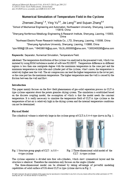
Numerical Simulation of Temperature Field in the CycloneZhenwei Zhang1, a, Ying Yu2,b, Jie Leng3,c and Sujuan Zhang4,d1School of Mechanical Engineering and Automation, Northeastern University, Shenyang, Liaoning,110819, China2Shenyang Nonferrous Metallurgy Engineering & Research Institute, Shenyang, Liaoning, 110003,China3Northeast Electric Power Research Institute Co., LTD, Shenyang, Liaoning, 110006, China 4Shenyang Agriculture University, Shenyang, Liaoning, 110866, Chinaa zzw1658@, b164038019@, c GLSLJ000000@, d130********@ Keywords: Separator, Numerical Simulation, Temperature Field.Abstract. The temperature distribution of the cyclone was analyzed in the presented work, which was imitated by using RSM turbulence model of software FLUENT. Temperature difference in different regions is less than one centigrade degree with the maximum temperature in the cone part and the minimum temperature in inlet tube and cylinder part of the cyclone, what’s more, the temperature is relatively higher near the wall. The air compression can lead the higher temperature in the lower part, so the cone part has the maximum temperature. The higher temperature near the wall is caused by the friction between the wall and flow.IntroductionThis paper mainly focuses on the flow field phenomenon of gas-solid separation process in CLT/A type cyclone separator about the potato granules drying system. The simulation is established based on the discrete coupling model, the assumption of which is that the model needs the constant temperature. It is really necessary to simulate the temperature field of CLT/A type cyclone as the temperature of hot air is relatively high in the drying system and the internal temperature conditions can not be determined.Physical ModelThe cylindrical volume is relatively large in the cyclone group of CLT/A 8.4×4 type shown in Fig. 1. Fig. 1 Structure group graph of CLT / A 8.0 ×4-type cycloneFig. 2 Three-dimensional solid model of theCLT / A-type cycloneThe cyclone separator is divided into four sub-cylinders, which show symmetrical layout and the structure is identical. Therefore the simulation only focuses on the single cylinder.The three-dimensional model can be obtained by taking advantage of powerful modeling capabilities of solid surface of UG about CLT/A type cyclone shown in Fig. 2.Finite Element ModelThe three-dimensional solid model established by UG can be imported into GAMBIT so as to be meshed. Multiple Boolean operations should be carried out on the solid model in order to be facilitated to mesh in GAMBIT, which can lead to the establishment of two entities form. The overall body of Volom1 is consisted of exhaust volute and exhaust pipe. The overall body of Volom2 is consisted of entrance pipe and cone below the cylinder. Then the model will be imported into GAMBIT with the total model shown in Fig. 3. The operations in GAMBIT can be shown as flowing.Fig. 3 Physical model of cyclone in GAMBIT Fig. 4 Mesh diagram of CLT / A-type cyclone(1) Establish the auxiliary plane and split the intake pipe with the Split command.(2) The cylinder can be divided into two parts with a plane parallel to Y-axis at Y=2260mm, the upper of which is ring cylinder with the lower part is cylinder.The entire cyclone is divided into four parts: intake pipe, outtake pipe, lower half part of the cylinder and the upper half part of the cylinder. The meshing can be imposed on them separately. Meshing is the premise process of numerical simulation and also the discrete process of calculating region. The number of the grid has little effect on the simulation result by continuing encryption , when the intensity of the grid reaches a certain value[1]. However, in practice, if the mesh is too sparse, it is so difficult to describe some detail in the flow field, what’s more, the computing speed can be greatly affected if the number of the meshing is too large. Therefore the number select of the grids can both guarantee the accuracy requirements and avoid excessive consumption of the system resources [2]. This paper adopts the complex grids according to the complexity of the flow field and variability of local feature. The hexahedral grid can be generated, which is the main structure, by taking advantage of Hex/Wedge-type structured grid and Cooper barrel pattern. This kind of grid matches well with the flow field, and is conductive to process of coupling conditions in the numerical simulation region. The meshing can be drawn as Fig. 4.Boundary ConditionsThe gas phase can be simplified in order to facilitate solving the multiphase flow inside the cyclone[3].(1) Gas flow is steady-state in cyclone;(2) The gas flow rate is low( generally less than 30m/s), and the gas can be seen as incompressible fluid;(3) The inlet air flows evenly, and in a fully developed turbulent state;(4) No gas exhausts from the dust exhaust at the bottom of the cyclone.Boundary conditions set as following:(1) Inlet boundary: the inlet air temperature is 373.3K, and the density is 1.225Kg/m3. The viscosity is 18.1×10⁻⁶ . Assuming that the inlet turbulent is developed fully, and the gas inlet velocity is set as 15m/s evenly distribution throughout the inlet section. The turbulence intensity is set as I and the hydraulic diameter is set as D. Flow Reynolds number is shown as Eq. 1.4e 61.225150.252R 2.5725101810UD ρµ−××===×× (1)Hydraulic diameter is set as Eq. 2.220.460.2070.2940.460.207HD ab D a b ××===++ (2) Turbulence Intensity is set as Eq. 3.1/851/8e 0.16(R )100%0.16(2.5710)7.34%I −−=×=××= (3)(2) Outlet boundary: outlet boundary is set as outflow boundary. Assuming that the flow condition is in fully developed condition, namely the flow situation can be obtained by the pulling of flow field. The air exhaust can be set as the outflow, and the weight of the flow is set as one. The dust exhaust is set as outflow, and the weight of the flow is set as zero.(3) Wall conditions: take the standard wall function, namely the wall has no-slip boundary [4]. The roughness parameter of wall is set as 0.5.(4) The overlapping circle is set as interface surface, which connects the exhaust pipe and cylinder. Numerical Simulation AnalysisTemperature distribution at various locations in CLT/A type cyclone can be intuitively obtained through numerical simulation shown in the Fig. 5. The entrance temperature is relatively low, and temperature can increase with moving downward along the cone. The value can reach the highest at the bottom of cone. The exhaust temperature can decrease along the exhaust pipe, but is still higher than inlet air temperature. The temperature change reason is shown as following: the air enters the air intake with the number of 100, and the flow can be compressed by centrifugal force caused by the rotation. In addition, the temperature can be increased due to the friction between the flow and wall. The temperature continues to rise owing to the further impact of compression and friction when reaches the cone wall.Fig. 6 and Fig. 7 respectively show the temperature distribution in Y=0 section about moderate and total temperature in CLT/A type cyclone separator. The moderate temperature distribution has the same situation with the total temperature distribution in the Y=0 cross section in the cyclone. The temperature of air intake and cylinder is the lowest with the maximum temperature in the cone part, and the temperature of exhaust pipe stays centre. The exhaust pipe temperature can decrease further. Temperature distribution shows a symmetrical situation in both sides of the exhaust pipe or inside it in cyclone with only little difference near the wall, which shows the vortex shape. The small difference is caused by the local turbulence accompanied by the rotation flow inside cyclone.Fig. 5 Total temperature field Fig. 6 Y=0 Static temperature Fig. 7 Y=0 Total temperature Fig. 8 and Fig. 9 respectively show the temperature distribution in X=0 section about static and total temperature in CLT/A type cyclone separator. Internal temperature distribution of X=0 section has the same situation with the total temperature distribution in cyclone. The cylinder part below the exhaust pipe has almost the same temperature distribution with the lower cone compared with the section Y=0 with only obvious difference in the position above the air exhaust, the reason for which is that the asymmetry caused the flow’s entrance from the unilateral line.Fig. 8 X=0 Static temperature Fig. 9 X=0 Total temperatureFig. 10 The temperature distribution on Z = 0.5, 0.75, 1, 1.25, 1.5, 1.75, 2 cross section Fig. 10 shows that temperature near the wall is relatively high, the reason for which is that friction between the flow and wall and compression effect of centrifugal force can lead the enhancement of temperature. Temperature gradient of each cross-section shows circular ring, better symmetry and a certain degree irregularity that can be caused by the different local turbulence.ConclusionThis thesis puts forward the temperature distribution of the cyclone with type of CLT/A, and figures out that the overall temperature is about 373°C. Temperature difference in different region is less than one centigrade degree with the maximum temperature in the cone part and the minimum temperature in inlet tube and cylinder part of the cyclone, what’s more, the temperature is relatively higher near the wall. The air compression can lead the higher temperature in the lower part, so the cone part has the maximum temperature which is caused by the strengthen impact of air compression. The higher temperature near the wall is caused by the friction between the wall and flow. The total temperature in the cyclone stays a constant value with almost no change and local difference can be obtained. Reference[1] F. Boysan, J. Ewan and B. Swithen. Experimental and Theoretical Studies of Cyclone SeparatorAerodynamics: (Chem E Symp Series, PP. 305-320, 1983).[2] W. Q. Tao. Modern Process of Heat Transfer Calculation: (Science Press, 2002).[3] G. L. Gao. Thermal Engineering and Fluid Mechanics: (China Electric Power Press, PP. 130-131, China 1997).[4] Y. Mao, L. Pang, X. W. Wang et al. Numerical Simulation of Three-dimensional Turbulence inCyclone: (Petroleum Refining and Chemical Industry, V. 33(2), PP. 1-6, China 2002).。

数模德尔菲法的英文名称《The Delphi Method in Numerical Modeling》The Delphi Method is a widely used research technique that is particularly valuable in the field of numerical modeling. This method involves obtaining input from a panel of experts to reach consensus on a particular topic or issue. The process typically involves multiple rounds of questionnaires and feedback, and is designed to distill the collective wisdom of the experts involved.In the context of numerical modeling, the Delphi Method can be a powerful tool for gathering insights from experts in various fields such as mathematics, computer science, and engineering. This input can be used to refine and improve the mathematical and computational models used to simulate complex systems and phenomena. By leveraging the knowledge and experience of a diverse group of experts, the Delphi Method can help ensure that the numerical models developed are accurate, reliable, and practical.The application of the Delphi Method in numerical modeling can lead to more robust and effective models, which in turn can have far-reaching implications in fields such as weather forecasting, structural engineering, and fluid dynamics. By leveraging the collective intelligence of a panel of experts, researchers and practitioners can gain valuable insights into the intricacies of the systems they are modeling, and develop more accurate and insightful predictions.In conclusion, the Delphi Method in numerical modeling holds great promise for improving the quality and reliability of mathematical and computational models. By harnessing the wisdom and expertise of a diverse group of experts, researchers and practitioners can develop more accurate and practical models that have the potential to revolutionize the way we understand and interact with the world around us.。

哈密尔顿系统的辛几何算法哈密尔顿系统是一类具有特殊的物理意义的动力系统,其在物理学、力学、动力学和计算力学等领域有着广泛应用。
哈密尔顿系统通常具有一组关于位置和动量的相变量,其演化满足哈密尔顿方程。
由于哈密尔顿系统具有良好的保持量和结构稳定性,因此在数值模拟中的算法设计尤其重要。
辛几何算法是一类特殊的数值演化方法,其以保持哈密尔顿系统相变量守恒和辛结构稳定性为目标,常常用于哈密尔顿系统的数值积分。
辛几何算法最早由李约瑟于 1988 年提出,其不仅能够在数值计算中保持相变量的守恒,还能够在哈密尔顿系统的长期演化中保持辛结构稳定性。
辛几何算法主要由两个部分组成,即辛映射和辛算子。
辛映射指的是从一个相变量向下一个相变量的映射,它通常满足“保相量”和辛结构不变性的特点。
保相量指的是相变量在变化过程中的守恒,而辛结构不变性则指的是哈密尔顿系统在演化过程中的辛不变性。
而辛算子则是这个辛映射的数值逼近,常常采用辛波发方法、显式和隐式辛算法等方法。
在演化哈密尔顿系统时,辛几何算法通常采用显式辛算法进行数值模拟。
显式辛算法的主要思路是采用辛映射和辛算子的组合,来实现对哈密尔顿系统的数值模拟。
在模拟过程中,辛几何算法需要保证每一步的演化都是辛的,这样系统才能保持哈密尔顿量以及其他相变量不变。
因此,辛几何算法在数值模拟中的应用非常广泛。
然而,辛几何算法的实现却比较困难。
在数值模拟时,辛几何算法需要考虑一系列问题,如相变量的数值守恒、哈密尔顿量的捕获和重构、快速演化、长时间演化、难以计算的高维效应等等。
这些问题都需要采用一些特殊的技巧和策略来解决。
总的来说,辛几何算法是一种特殊的数值演化方法,其以保持哈密尔顿系统相变量守恒和辛结构稳定性为目标,在计算力学、物理学、动力学等领域有着广泛应用。
黎曼猜想英语The Riemann Hypothesis, named after the 19th-century mathematician Bernhard Riemann, is one of the most profound and consequential conjectures in mathematics. It is concerned with the distribution of the zeros of the Riemann zeta function, a complex function denoted as $$\zeta(s)$$, where $$s$$ is a complex number. The hypothesis posits that all non-trivial zeros of this analytical function have their real parts equal to $$\frac{1}{2}$$.To understand the significance of this conjecture, one must delve into the realm of number theory and the distribution of prime numbers. Prime numbers are the building blocks of arithmetic, as every natural number greater than 1 is either a prime or can be factored into primes. The distribution of these primes, however, has puzzled mathematicians for centuries. The Riemann zeta function encodes information about the distribution of primes through its zeros, and thus, the Riemann Hypothesis is directly linked to understanding this distribution.The zeta function is defined for all complex numbers except for $$s = 1$$, where it has a simple pole. For values of $$s$$ with a real part greater than 1, it converges to a sum over the positive integers, as shown in the following equation:$$\zeta(s) = \sum_{n=1}^{\infty} \frac{1}{n^s}$$。
聚类和异常值分析与热点分析
前面我们聊的各种指数,无论是莫兰指数还是P值Z得分,都是整体数据的结论,也就是所谓“全局莫兰指数( Globe Moran'sI)" , 也就说,不管我给你多少数据,最后你就吐出一个来给我!这算神马!当然,从名字上来看, 全局数据嘛,有一个给你就不错了。
实际上作为我们玩GIS的人,最喜欢的就是出一张花花绿绿的地图, 比如这样的, 或者是这样的:所以我们更希望的是将我们输入的数据,标示出明显的数值来,比如我输入1000个要素,那么你别就给我1个数据啊,怎么也得吐出1000个数据来吧, 甭管什么莫兰指数, P值Z得分啥的,不能给我省了。
所以这里就要用到今天我们说的Anselin LocalMoran's I方法了,而它与GlobeMoran's I的区别, 如下:所以,这种算法比较符合我们做GIS的人的思维,那么这种可视为地理信息强迫症的特效药的Anselin Local Moran's I算法,是哪位大爷提出来的呢?
下面进入我们的算法科普时间:
上面这个脑[ ]像土豆神一样明亮的老帅哥,就是ASU(美国亚利桑那州立大学)的地理与规划学院院长Luc Anselin教授,也是Anselin Local Moran'I算法的提出者,所以也就用了他的大名来标示这种算法。
如果做地理分析的,一定听说一个叫做GeoDa的软件,这个软件就是Anselin 教授领导的ASU的地理空间分析和计算中心弄出来的神器。
后来他的这个中心,就一直被人称为"GeoDa Center".。
cfd中的asymptotic theory[cfd中的asymptotic theory]Asymptotic theory plays a vital role in Computational Fluid Dynamics (CFD) as it provides a mathematical framework to understand the behavior of fluid flow in various situations. In this article, we will explore the fundamentals of asymptotic theory in CFD and its applications.What is asymptotic theory?Asymptotic theory is a branch of mathematics that deals with the behavior of functions as a variable approaches a particular value. It provides a systematic way to approximate complex functions and simplify their analysis. In CFD, asymptotic theory is used to solve fluid flow problems by approximating complex equations and simplifying their solutions.The foundation of asymptotic theory in CFD lies in the concept of a small parameter. A small parameter is a dimensionless quantity that represents the scale of a physical phenomenon relative to other quantities in the problem. It allows us to analyze thebehavior of the fluid flow as the small parameter tends to zero or infinity.The key idea behind asymptotic theory is that we can approximate the solution to a problem by expanding it as a series in powers of the small parameter. The resulting series is then truncated at an appropriate order to obtain an approximate solution. This approach is particularly useful when the problem involves a wide range of scales, such as in turbulent flows or flows with thin boundary layers.Applications of asymptotic theory in CFD1. Boundary layer theory: Boundary layers are thin layers of fluid that form near solid boundaries in a fluid flow. They play a crucial role in many engineering applications, such as aerodynamics and heat transfer. Asymptotic theory allows us to derive simplified equations for the boundary layer and study its behavior.By assuming the small parameter to be the ratio of the boundary layer thickness to the characteristic length scale of the problem, we can derive the famous Prandtl's boundary layer equations.These equations provide a simplified description of the flow near the boundary and have been widely used to analyze various flow problems.2. Perturbation methods: Perturbation methods involve solving a problem by treating the small parameter as a small perturbation to an already known solution. This approach is particularly useful when the small parameter is not related to a physical scale but appears in the governing equations due to simplifications or assumptions.For example, in the study of unsteady flows, the small parameter can be the ratio of the unsteadiness time scale to a characteristic time scale of the problem. By assuming a known steady solution and perturbing it in terms of the small parameter, we can develop a systematic procedure to obtain the unsteady solution.3. Homogenization theory: Homogenization theory is concerned with problems where the governing equations have oscillatory coefficients or rapidly varying parameters. These problems arise in various fields, such as porous media flow and composite materials.Asymptotic theory provides a powerful tool to derive effective (homogenized) equations that capture the behavior of the system on a macroscopic scale. By assuming the small parameter as the ratio of the periodicity length to the characteristic length scale of the problem, we can develop an asymptotic expansion to obtain the macroscopic equations.ConclusionAsymptotic theory is an essential tool in CFD for studying complex fluid flow problems. It allows us to approximate the solution to a problem by expanding it as a series in powers of a small parameter and truncating the series at an appropriate order. This approach provides simplified equations that capture the essential behavior of the flow and enable efficient computational analysis. Through examples such as boundary layer theory, perturbation methods, and homogenization theory, we have seen how asymptotic theory finds applications in various areas of CFD. By using asymptotic theory, researchers can gain valuable insights into the behavior of fluid flow and develop efficient numericalmethods for practical engineering applications.。