Using Local Optimization in Surface Fitting To appear in Mathematical Methods for Curves an

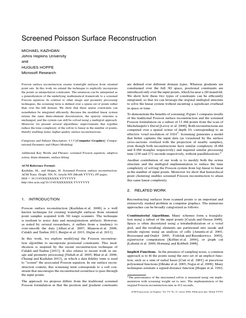
Screened Poisson Surface ReconstructionMICHAEL KAZHDANJohns Hopkins UniversityandHUGUES HOPPEMicrosoft ResearchPoisson surface reconstruction creates watertight surfaces from oriented point sets.In this work we extend the technique to explicitly incorporate the points as interpolation constraints.The extension can be interpreted as a generalization of the underlying mathematical framework to a screened Poisson equation.In contrast to other image and geometry processing techniques,the screening term is defined over a sparse set of points rather than over the full domain.We show that these sparse constraints can nonetheless be integrated efficiently.Because the modified linear system retains the samefinite-element discretization,the sparsity structure is unchanged,and the system can still be solved using a multigrid approach. Moreover we present several algorithmic improvements that together reduce the time complexity of the solver to linear in the number of points, thereby enabling faster,higher-quality surface reconstructions.Categories and Subject Descriptors:I.3.5[Computer Graphics]:Compu-tational Geometry and Object ModelingAdditional Key Words and Phrases:screened Poisson equation,adaptive octree,finite elements,surfacefittingACM Reference Format:Kazhdan,M.,and Hoppe,H.Screened Poisson surface reconstruction. ACM Trans.Graph.NN,N,Article NN(Month YYYY),PP pages.DOI=10.1145/XXXXXXX.YYYYYYY/10.1145/XXXXXXX.YYYYYYY1.INTRODUCTIONPoisson surface reconstruction[Kazhdan et al.2006]is a well known technique for creating watertight surfaces from oriented point samples acquired with3D range scanners.The technique is resilient to noisy data and misregistration artifacts.However, as noted by several researchers,it suffers from a tendency to over-smooth the data[Alliez et al.2007;Manson et al.2008; Calakli and Taubin2011;Berger et al.2011;Digne et al.2011].In this work,we explore modifying the Poisson reconstruc-tion algorithm to incorporate positional constraints.This mod-ification is inspired by the recent reconstruction technique of Calakli and Taubin[2011].It also relates to recent work in im-age and geometry processing[Nehab et al.2005;Bhat et al.2008; Chuang and Kazhdan2011],in which a datafidelity term is used to“screen”the associated Poisson equation.In our surface recon-struction context,this screening term corresponds to a soft con-straint that encourages the reconstructed isosurface to pass through the input points.The approach we propose differs from the traditional screened Poisson formulation in that the position and gradient constraints are defined over different domain types.Whereas gradients are constrained over the full3D space,positional constraints are introduced only over the input points,which lie near a2D manifold. We show how these two types of constraints can be efficiently integrated,so that we can leverage the original multigrid structure to solve the linear system without incurring a significant overhead in space or time.To demonstrate the benefits of screening,Figure1compares results of the traditional Poisson surface reconstruction and the screened Poisson formulation on a subset of11.4M points from the scan of Michelangelo’s David[Levoy et al.2000].Both reconstructions are computed over a spatial octree of depth10,corresponding to an effective voxel resolution of10243.Screening generates a model that better captures the input data(as visualized by the surface cross-sections overlaid with the projection of nearby samples), even though both reconstructions have similar complexity(6.8M and6.9M triangles respectively)and required similar processing time(230and272seconds respectively,without parallelization).1 Another contribution of our work is to modify both the octree structure and the multigrid implementation to reduce the time complexity of solving the Poisson system from log-linear to linear in the number of input points.Moreover we show that hierarchical point clustering enables screened Poisson reconstruction to attain this same linear complexity.2.RELA TED WORKReconstructing surfaces from scanned points is an important and extensively studied problem in computer graphics.The numerous approaches can be broadly categorized as follows. Combinatorial Algorithms.Many schemes form a triangula-tion using a subset of the input points[Cazals and Giesen2006]. Space is often discretized using a tetrahedralization or a voxel grid,and the resulting elements are partitioned into inside and outside regions using an analysis of cells[Amenta et al.2001; Boissonnat and Oudot2005;Podolak and Rusinkiewicz2005], eigenvector computation[Kolluri et al.2004],or graph cut [Labatut et al.2009;Hornung and Kobbelt2006].Implicit Functions.In the presence of sampling noise,a common approach is tofit the points using the zero set of an implicit func-tion,such as a sum of radial bases[Carr et al.2001]or piecewise polynomial functions[Ohtake et al.2005;Nagai et al.2009].Many techniques estimate a signed-distance function[Hoppe et al.1992; 1The performance of the unscreened solver is measured using our imple-mentation with screening weight set to zero.The implementation of the original Poisson reconstruction runs in412seconds.ACM Transactions on Graphics,V ol.VV,No.N,Article XXX,Publication date:Month YYYY.2•M.Kazhdan and H.HoppeFig.1:Reconstruction of the David head ‡,comparing traditional Poisson surface reconstruction (left)and screened Poisson surface reconstruction which incorporates point constraints (center).The rightmost diagram plots pixel depth (z )values along the colored segments together with the positions of nearby samples.The introduction of point constraints significantly improves fit accuracy,sharpening the reconstruction without amplifying noise.Bajaj et al.1995;Curless and Levoy 1996].If the input points are unoriented,an important step is to correctly infer the sign of the resulting distance field [Mullen et al.2010].Our work extends Poisson surface reconstruction [Kazhdan et al.2006],in which the implicit function corresponds to the model’s indicator function χ.The function χis often defined to have value 1inside and value 0outside the model.To simplify the derivations,inthis paper we define χto be 12inside and −12outside,so that its zero isosurface passes near the points.The function χis solved using a Laplacian system discretized over a multiresolution B-spline basis,as reviewed in Section 3.Alliez et al.[2007]form a Laplacian system over a tetrahedral-ization,and constrain the solution’s biharmonic energy;the de-sired function is obtained as the solution to an eigenvector prob-lem.Manson et al.[2008]represent the indicator function χusing a wavelet basis,and efficiently compute the basis coefficients using simple local sums over an adapted octree.Calakli and Taubin [2011]optimize a signed-distance function to have value zero at the points,have derivatives that agree with the point normals,and minimize a Hessian smoothness norm.The resulting optimization involves a bilaplacian operator,which requires estimating derivatives of higher order than in the Laplacian.The reconstructed surfaces are shown to have good accuracy,strongly suggesting the importance of explicitly fitting the points within the optimization.This motivated us to explore whether a Laplacian system could be extended in this respect,and also be compatible with a multigrid solver.Screened Poisson Surface Fitting.The method of Nehab et al.[2005],which simultaneously fits position and normal constraints,may also be viewed as the solution of a screened Poisson equation.The fitting algorithm assumes that a 2D parametric domain (i.e.,a plane or triangle mesh)is already established.The position and derivative constraints are both defined over this 2D domain.In contrast,in Poisson surface reconstruction the 2D domain manifold is initially unknown,and therefore the goal is to infer anindicator function χrather than a parametric function.This leadsto a hybrid problem with derivative (Laplacian)constraints defined densely over 3D and position constraints defined sparsely on the set of points sampled near the unknown 2D manifold.3.REVIEW OF POISSON SURFACE RECONSTRUCTIONThe approach of Poisson surface reconstruction is based on the observation that the (inward pointing)normal field of the boundary of a solid can be interpreted as the gradient of the solid’s indicator function.Thus,given a set of oriented points sampling the boundary,a watertight mesh can be obtained by (1)transforming the oriented point samples into a continuous vector field in 3D,(2)finding a scalar function whose gradients best match the vector field,and (3)extracting the appropriate isosurface.Because our work focuses primarily on the second step,we review it here in more detail.Scalar Function Fitting.Given a vector field V :R 3→R 3,thegoal is to solve for the scalar function χ:R 3→R minimizing:E (χ)=∇χ(p )− V (p ) 2d p .(1)Using the Euler-Lagrange formulation,the minimum is obtainedby solving the Poisson equation:∆χ=∇· V .System Discretization.The Galerkin formulation is used totransform this into a finite-dimensional system [Fletcher 1984].First,a basis {B 1,...,B N }:R 3→R is chosen,namely a collection of trivariate (usually triquadratic)B-spline functions.With respect to this basis,the discretization becomes:∆χ,B i [0,1]3= ∇· V ,B i [0,1]31≤i ≤Nwhere ·,· [0,1]3is the standard inner-product on the space of(scalar-and vector-valued)functions defined on the unit cube:F ,G [0,1]3=[0,1]3F (p )·G (p )d p , U , V [0,1]3=[0,1]3U (p ), V (p ) d p .Since the solution is itself expressed in terms of the basis functions:χ(p )=N∑i =1x i B i (p ),ACM Transactions on Graphics,V ol.VV ,No.N,Article XXX,Publication date:Month YYYY .1.离散化->连续2.找个常量函数最佳拟合这些这些向量域;3.抽取等值面这里已经将离散的有向点转化为了连续的向量域表示;点集合的最初的思考Screened Poisson Surface Reconstruction•3finding the coefficients{x i}of the solution reduces to solving the linear system Ax=b where:A i j= ∇B i,∇B j [0,1]3and b i= V,∇B i [0,1]3.(2) The basis functions{B1,...,B N}are chosen to be compactly supported,so most pairs of functions do not have overlapping support,and thus the matrix A is sparse.Because the solution is expected to be smooth away from the input samples,the linear system is discretized byfirst adapting an octree to the input samples and then associating an(appropriately scaled and translated)trivariate B-spline function to each octree node. This provides high-resolution detail in the vicinity of the surface while reducing the overall dimensionality of the system.System Solution.Given the hierarchy defined by an octree of depth D,a multigrid approach is used to solve the linear system. The basis functions are partitioned according to the depths of their associated nodes and,for each depth d,a linear system A d x d=b d is defined using the corresponding B-splines{B d1,...,B d Nd},such thatχ(p)=∑D d=0∑i x d i B d i(p).Because the octree-selected B-spline functions do not form a complete grid at each depth,it is generally not possible to prolong the solution x d at depth d into the solution x d+1at depth d+1. (The B-spline associated with a given node is a sum of B-spline functions associated not only with its own child nodes,but also with child nodes of its neighbors.)Instead,the constraints at depth d+1are adjusted to account for the part of the solution already realized at coarser depths.Pseudocode for a cascadic solver,where the solution is only relaxed on the up-stroke of the V-cycle,is given in Algorithm1.Algorithm1:Cascadic Poisson Solver1For d∈{0,...,D}Iterate from coarse tofine2For d ∈{0,...,d−1}Remove the constraints3b d=b d−A dd x d met at coarser depths4Relax A d x d=b d Adjust the system at depth dHere,A dd is the N d×N d matrix used to transform solution coefficients at depth d into constraints at depth d:A dd i j= ∇B d i,∇B d j [0,1]3.Note that,by definition,A d=A dd.Isosurface Extraction.Solving the Poisson equation,one obtains a functionχthat approximates the indicator function.Ideally,the function’s zero level-set should therefore correspond to the desired surface.In practice however,the functionχcan differ from the true indicator function due to several sources of error:—The point sampling may be noisy,possibly containing outliers.—The Galerkin discretization is only an approximation of the continuous problem.—The point sampling density is approximated during octree construction.To mitigate these errors,in[Kazhdan et al.2006]the implicit function is adjusted by globally subtracting the average value of the function at the input samples.4.INCORPORA TING POINT CONSTRAINTSThe original Poisson surface reconstruction algorithm adjusts the implicit function using a single global offset such that its average value at all points is zero.However,the presence of errors can cause the implicit function to drift so that no global offset is satisfactory. Instead,we seek to explicitly interpolate the points.Given the set of input points P with weights w:P→R≥0,we add to the energy of Equation1a term that penalizes the function’s deviation from zero at the samples:E(χ)=V(p)−∇χ(p) 2d p+α·Area(P)∑p∈P∑p∈Pw(p)χ2(p)(3)whereαis a weight that trades off the importance offitting the gradients andfitting the values,and Area(P)is the area of the reconstructed surface,estimated by computing the local sampling density as in[Kazhdan et al.2006].In our implementation,we set the per-sample weights w(p)=1,although one can also use confidence values if these are available.The energy can be expressed concisely asE(χ)= V−∇χ, V−∇χ [0,1]3+α χ,χ (w,P)(4)where ·,· (w,P)is the bilinear,symmetric,positive,semi-definite form on the space of functions in the unit-cube,obtained by taking the weighted sum of function values:F,G (w,P)=Area(P)∑p∈P w(p)∑p∈Pw(p)·F(p)·G(p).4.1Interpretation as a Screened Poisson EquationThe energy in Equation4combines a gradient constraint integrated over the spatial domain with a value constraint summed at discrete points.As shown in the appendix,its minimization can be interpreted as a screened Poisson equation(∆−α˜I)χ=∇· V with an appropriately defined operator˜I.4.2DiscretizationWe apply a discretization similar to that in Section3to the minimization of the energy in Equation4.The coefficients of the solutionχwith respect to the basis{B1,...,B N}are again obtained by solving a linear system of the form Ax=b.The right-hand-side b is unchanged because the constrained value at the sample points is zero.Matrix A now includes the point constraints:A i j= ∇B i,∇B j [0,1]3+α B i,B j (w,P).(5) Note that incorporating the point constraints does not change the sparsity of matrix A because B i(p)·B j(p)is nonzero only if the supports of the two functions overlap,in which case the Poisson equation has already introduced a nonzero entry in the matrix.As in Section3,we solve this linear system using a cascadic multigrid algorithm–iterating over the octree depths from coarsest tofinest,adjusting the constraints,and relaxing the system.Similar to Equation5,the matrix used to transform a solution at depth d to a constraint at depth d is expressed as:A dd i j= ∇B d i,∇B d j [0,1]3+α B d i,B d j (w,P).ACM Transactions on Graphics,V ol.VV,No.N,Article XXX,Publication date:Month YYYY.4•M.Kazhdan and H.HoppeFig.2:Visualizations of the reconstructed implicit function along a planar slice through the cow ‡(shown in blue on the left),for the original Poisson solver,and for the screened Poisson solver without and with scale-independent screening.This operator adjusts the constraint b d (line 3of Algorithm 1)not only by removing the Poisson constraints met at coarser resolutions,but also by modifying the constrained values at points where the coarser solution does not evaluate to zero.4.3Scale-Independent ScreeningTo balance the two energy terms in Equation 3,it is desirable to adjust the screening parameter αsuch that (1)the reconstructed surface shape is invariant under scaling of the input points with respect to the solver domain,and (2)the prolongation of a solution at a coarse depth is an accurate estimate of the solution at a finer depth in the cascadic multigrid approach.We achieve both these goals by adjusting the relative weighting of position and gradient constraints across the different octree depths.Noting that the magnitude of the gradient constraint scales with resolution,we double the weight of the interpolation constraint with each depth:A ddi j = ∇B d i ,∇B dj [0,1]3+2d α B d i ,B dj (w ,P ).The adaptive weight of 2d is chosen to keep the Laplacian and screening constraints around the surface in balance.To see this,assume that the points are locally planar,and consider the row of the system matrix corresponding to an octree node overlapping the points.The coefficients of the system in that row are the sum of Laplacian and screening terms.If we consider the rows corresponding to the child nodes that overlap the surface,we find that the contribution from the Laplacian constraints scales by a factor of 1/2while the contribution from the screening term scales by a factor of 1/4.2Thus,scaling the screening weights by a factor of two with each resolution keeps the two terms in balance.Figure 2shows the benefit of scale-independent screening in reconstructing a cow model.The leftmost image shows a plane passing through the bounding cube of the cow,and the images to the right show the values of the computed indicator function along that plane,for different implementations of the solver.As the figure shows,the unscreened Poisson solver provides a good approximation of the indicator functions,with values inside (resp.outside)the surface approximately 1/2(resp.-1/2).However,applying the same solver to the screened Poisson equation (second from right)provides a solution that is only correct near the input samples and returns to zero near the faces of the bounding cube,2Forthe Laplacian term,the Laplacian scales by a factor of 4with refinement,and volumetric integrals scale by a factor of 1/8.For the screening term,area integrals scale by a factor of 1/4.potentially resulting in spurious surface sheets away from the surface.It is only with scale-independent screening (right)that we obtain a high-quality solution to the screened Poisson ing this resolution adaptive weighting,our system has the property that the reconstruction obtained by solving at depth D is identical to the reconstruction that would be obtained by scaling the point set by 1/2and solving at depth D +1.To see this,we consider the two energies that guide the reconstruc-tion,E V (χ)measuring the extent to which the gradients of the so-lution match the prescribed vector field,and E (w ,P )(χ)measuring the extent to which the solution meets the screening constraint:E V (χ)=V (p )−∇χ(p )2d p E (w ,P )(χ)=Area (P )∑p ∈P w (p )∑p ∈Pw (p )χ2(p ).Scaling by 1/2,we obtain a new point set (˜w ,˜P)with positions scaled by 1/2,unchanged weights,˜w (p )=w (2p ),and scaled area,Area (˜P )=Area (P )/4;a new scalar field,˜χ(p )=χ(2p );and a new vector field,˜ V (p )=2 V (2p ).Computing the correspondingenergies,we get:E ˜ V (˜χ)=1E V(χ)and E (˜w ,˜P )(˜χ)=1E (w ,P )(χ).Thus,scaling the screening weight by a factor of two with eachsuccessive depth ensures that the sum of energies is unchanged (up to multiplication by a constant)so the minimizer remains the same.4.4Boundary ConditionsIn order to define the linear system,it is necessary to define the behavior of the function space along the boundary of the integration domain.In the original Poisson reconstruction the authors imposed Dirichlet boundary conditions,forcing the implicit function to havea value of −12along the boundary.In the present work we extend the implementation to support Neumann boundary conditions as well,forcing the normal derivative to be zero along the boundary.In principle these two boundary conditions are equivalent for watertight surfaces,since the indicator function has a constant negative value outside the model.However,in the presence of missing data we find Neumann constraints to be less restrictive because they only require that the implicit function have zero derivative across the boundary of the integration domain,a property that is compatible with the gradient constraint since the guiding vector field V is set to zero away from the samples.(Note that when the surface does cross the boundary of the domain,the Neumann boundary constraints create a bias to crossing the domain boundary orthogonally.)Figure 3shows the practical implications of this choice when reconstructing the Angel model,which was only scanned from the front.The left image shows the original point set and the reconstructions using Dirichlet and Neumann boundary conditions are shown to the right.As the figure shows,imposing Dirichlet constraints creates a water-tight surface that closes off before reaching the boundary while using Neumann constraints allows the surface to extend out to the boundary of the domain.ACM Transactions on Graphics,V ol.VV ,No.N,Article XXX,Publication date:Month YYYY .Screened Poisson Surface Reconstruction•5Fig.3:Reconstructions of the Angel point set‡(left)using Dirichlet(center) and Neumann(right)boundary conditions.Similar results can be seen at the bases of the models in Figures1 and4a,with the original Poisson reconstructions obtained using Dirichlet constraints and the screened reconstructions obtained using Neumann constraints.5.IMPROVED ALGORITHMIC COMPLEXITYIn this section we discuss the efficiency of our reconstruction al-gorithm.We begin by analyzing the complexity of the algorithm described above.Then,we present two algorithmic improvements. Thefirst describes how hierarchical clustering can be used to re-duce the screening overhead at coarser resolutions.The second ap-plies to both the unscreened and screened solver implementations, showing that the asymptotic time complexity in both cases can be reduced to be linear in the number of input points.5.1Efficiency of basic solverLet us begin by analyzing the computational complexity of the unscreened and screened solvers.We assume that the points P are evenly distributed over a surface,so that the depth of the adapted octree is D=O(log|P|)and the number of octree nodes at depth d is O(4d).We also note that the number of nonzero entries in matrix A dd is O(4d),since the matrix has O(4d)rows and each row has at most53nonzero entries.(Since we use second-order B-splines, basis functions are supported within their one-ring neighborhoods and the support of two functions will overlap only if one is within the two-ring neighborhood of the other.)Assuming that the matrices A dd have already been computed,the computational complexity for the different steps in Algorithm1is: Step3:O(4d)–since A dd has O(4d)nonzero entries.Step4:O(4d)–since A d has O(4d)nonzero entries and the number of relaxation steps performed is constant.Steps2-3:∑d−1d =0O(4d)=O(4d·d).Steps2-4:O(4d·d+4d)=O(4d·d).Steps1-4:∑D d=0O(4d·d)=O(4D·D)=O(|P|·log|P|). There still remains the computation of matrices A dd .For the unscreened solver,the complexity of computing A dd is O(4d),since each entry can be computed in constant time.Thus, the overall time complexity remains O(|P|·log|P|).For the screened solver,the complexity of computing A dd is O(|P|)since defining the coefficients requires accumulating the screening contribution from each of the points,and each point contributes to a constant number of rows.Thus,the overall time complexity is dominated by the cost of evaluating the coefficients of A dd which is:D∑d=0d−1∑d =0O(|P|)=O(|P|·D2)=O(|P|·log2|P|).5.2Hierarchical Clustering of Point ConstraintsOurfirst modification is based on the observation that since the basis functions at coarser resolutions are smooth,it is unnecessary to constrain them at the precise sample locations.Instead,we cluster the weighted points as in[Rusinkiewicz and Levoy2000]. Specifically,for each depth d,we define(w d,P d)where p i∈P d is the weighted average position of the points falling into octree node i at depth d,and w d(p i)is the sum of the associated weights.3 If all input points have weight w(p)=1,then w d(p i)is simply the number of points falling into node i.This alters the computation of the system matrix coefficients:A dd i j= ∇B d i,∇B d j [0,1]3+2dα B d i,B d j (w d,P d).Note that since d>d ,the value B d i,B d j (w d,P d)is obtained by summing over points stored with thefiner resolution.In particular,the complexity of computing A dd for the screened solver becomes O(|P d|)=O(4d),which is the same as that of the unscreened solver,and both implementations now have an overall time complexity of O(|P|·log|P|).On typical examples,hierarchical clustering reduces execution time by a factor of almost two,and the reconstructed surface is visually indistinguishable.5.3Conforming OctreesTo account for the adaptivity of the octree,Algorithm1subtracts off the constraints met at all coarser resolutions before relaxing at a given depth(steps2-3),resulting in an algorithm with log-linear time complexity.We obtain an implementation with linear complexity by forcing the octree to be conforming.Specifically, we define two octree cells to be mutually visible if the supports of their associated B-splines overlap,and we require that if a cell at depth d is in the octree,then all visible cells at depth d−1must also be in the tree.Making the tree conforming requires the addition of new nodes at coarser depths,but this still results in O(4d)nodes at depth d.While the conforming octree does not satisfy the condition that a coarser solution can be prolonged into afiner one,it has the property that the solution obtained at depths{0,...,d−1}that is visible to a node at depth d can be expressed entirely in terms of the coefficients at depth d−ing an accumulation vector to store the visible part of the solution,we obtain the linear-time implementation in Algorithm2.3Note that the weight w d(p)is unrelated to the screening weight2d introduced in Section4.3for scale-independent screening.ACM Transactions on Graphics,V ol.VV,No.N,Article XXX,Publication date:Month YYYY.6•M.Kazhdan and H.HoppeHere,P d d−1is the B-spline prolongation operator,expressing a solution at depth d−1in terms of coefficients at depth d.The number of nonzero entries in P d d−1is O(4d),since each column has at most43nonzero entries,so steps2-5of Algorithm2all have complexity O(4d).Thus,the overall complexity of both the unscreened and screened solvers becomes O(|P|).Algorithm2:Conforming Cascadic Poisson Solver1For d∈{0,...,D}Iterate from coarse tofine.2ˆx d−1=P d−1d−2ˆx d−2Upsample coarseraccumulation vector.3ˆx d−1=ˆx d−1+x d−1Add in coarser solution.4b d=b d−A d d−1ˆx d−1Remove constraintsmet at coarser depths.5Relax A d x d=b d Adjust the system at depth d.5.4Implementation DetailsThe algorithm is implemented in C++,using OpenMP for multi-threaded parallelization.We use a conjugate-gradient solver to re-lax the system at each multigrid level.With the exception of the octree construction,most of the operations involved in the Poisson reconstruction can be categorized as operations that either“accu-mulate”or“distribute”information[Bolitho et al.2007,2009].The former do not introduce write-on-write conflicts and are trivial to parallelize.The latter only involve linear operations,and are par-allelized using a standard map-reduce approach:in the map phase we create a duplicate copy of the data for each thread to distribute values into,and in the reduce phase we merge the copies by taking their sum.6.RESULTSWe evaluate the algorithm(Screened)by comparing its accuracy and computational efficiency with several prior methods:the original Poisson reconstruction of Kazhdan et al.[2006](Poisson), the Wavelet reconstruction of Manson et al.[2008](Wavelet),and the Smooth Signed Distance reconstruction of Calakli and Taubin [2011](SSD).For the new algorithm,we set the screening weight toα=4and use Neumann boundary conditions in all experiments.(Numerical results obtained using Dirichlet boundaries were indistinguishable.) For the prior methods,we set algorithmic parameters to values recommended by the authors,using Haar Wavelets in the Wavelet reconstruction and setting the value/normal/Hessian weights to 1/1/0.25in the SSD reconstruction.For Poisson,SSD,and Screened we set the“samples-per-node”parameter to1and the “bounding-box-scale”parameter to1.1.(For Wavelet the bounding box scale is hard-coded at1and there is no parameter to adjust the sampling density.)6.1AccuracyWe run three different types of experiments.Real Scanner Data.To evaluate the accuracy of the different reconstruction algorithms on real-world data,we gathered several scanned datasets:the Awakening(10M points),the Stanford Bunny (0.2M points),the David(11M points),the Lucy(1.0M points), and the Neptune(2.4M points).For each dataset,we randomly partitioned the points into two equal-sized subsets:input points for the reconstruction algorithms,and validation points to measure point-to-reconstruction distances.Figure4a shows reconstructions results for the Neptune and David models at depth10.It also shows surface cross-sections overlaid with the validation points in their vicinity.These images reveal that the Poisson reconstruction(far left),and to a lesser extent the SSD reconstruction(center left),over-smooth the data,while the Wavelet reconstruction(center left)has apparent derivative discontinuities.In contrast,our screened Poisson approach(far right)provides a reconstruction that faithfullyfits the samples without introducing noise.Figure4b shows quantitative results across all datasets,in the form of RMS errors,measured using the distances from the validation points to the reconstructed surface.(We also computed the maximum error,but found that its sensitivity to individual outlier points made it an unreliable and unindicative statistic.)As thefigure indicates,the Screened Poisson reconstruction(blue)is always more accurate than both the original Poisson reconstruction algorithm(red)and the Wavelet reconstruction(purple),and generates reconstruction whose RMS errors are comparable to or smaller than those of the SSD reconstruction(green).Clean Uniformly Sampled Data.To evaluate reconstruction accuracy on clean data,we used the approach of Osada et al.[2001] to generate oriented point sets by uniformly sampling the surfaces of the Fandisk,Armadillo Man,Dragon,and Raptor models.For each model,we generated datasets of100K and1M points and reconstructed surfaces from each point set using the four different reconstruction algorithms.As an example,Figure5a shows the reconstructions of the fandisk and raptor models using1M point samples at depth10.Despite the lack of noise in the input data,the Wavelet reconstruction has spurious high-frequency detail.Focusing on the sharp edges in the model,we also observe that the screened Poisson reconstruction introduces less smoothing,providing a reconstruction that is truer to the original data than either the original Poisson or the SSD reconstructions.Figure5b plots RMS errors across all models,measured bidirec-tionally between the original surface and the reconstructed surface using the Metro tool[Cignoni and Scopigno1998].As in the case of real scanner data,screened Poisson reconstruction always out-performs the original Poisson and Wavelet reconstructions,and is comparable to or better than the SSD reconstruction. Reconstruction Benchmark.We use the benchmark of Berger et al.[2011]to evaluate the accuracy of the algorithms under different simulations of scanner error,including nonuniform sampling,noise,and misalignment.The dataset consists of mul-tiple virtual scans of implicit surfaces representing the Anchor, Dancing Children,Daratech,Gargoyle,and Quasimodo models. As an example,Figure6a visualizes the error in the reconstructions of the anchor model from a virtual scan consisting of210K points (demarked with a dashed rectangle in Figure6b)at depth9.The error is visualized using a red-green-blue scale,with red signifyingACM Transactions on Graphics,V ol.VV,No.N,Article XXX,Publication date:Month YYYY.。

Design Optimization in Pro/ENGINEER Wildfire 2.0January 18, 20051 IntroductionThe Structure and Thermal Analysis using FEA provide means to evaluate the stress, strain, and heat distributions within in a design model, given the working conditions, and materials.Using these analysis tools and other build-in performance measuring functions in Pro/E, a user defined design objective (or goal) can be measured. This objective is normally directly related by a number of design dimensions. Changing the values of these dimensions, or design variables, the value of the defined design objective will change accordingly. Design optimization is the tool that automatically search for the best values of these design variables, given the user defined design objectives. In most applications, a number of design constraints are also specified to design the boundaries of the allowed design variations.Design Optimization tool in Pro/E automatically adjusts one or several design parameters in a series of design-analysis iterations to move closer to the goal while satisfying any limits defined. It can also be used to test the feasibility of a design with respect to some specified constraints or limits. In these feasibility studies, no goal is defined; ProE simply tries to satisfy the pre-defined limits. The goal and limits are each optional, but a study must have at least one goal or one limit.In this tutorial, we use a gear and gear shaft design example to demonstrate the method of Design Optimization.We simplify the problem by assuming that the gear and shaft are one body made using steel, consider minimum weight as the goal of the design, and chose the width of the gear, d4, as design variable. Other known parameters include:Length ofShaft, d7=d1 Diameter of Shaft, d6=d0Diameter of Gear, d3 Initial Width of Gear, d4 Chamfer Radii d11=d128′′ 2′′ 10′′ 3′′ 0.125′′• Material is Steel.• Dimensions: d0, d1, d6, d7, d3, d11, d12 and total length of the part are fixed.• The part cannot bear a stress more than 8710×(22lbm s in) [von_Mises] • The part is fixed at both ends. • A work load, 77[110;0;110]F =××G (lb), is applied on the outer cylinder surfacerepresenting the gear.The design optimization is to be carried out to get the optimal value of the dimension d4 that allow the component to have a minimum weight.2 Model CreationIn this part, we create the geometry model and add mechanical properties to it.2.1 Create the Solid Model of the Gear-ShaftIn Pro/E, create the part as shown in the previous figure. Since we need to maintain the length ofthe shaft while adjusting the dimension d4, we add a dimension relation:d7=11-d42.2 Start Pro/E MechanicaTo begin Structure Analysis, in Pro/E, select:Application>MechanicaThen, assign material, add constraints, apply work load and mesh the model as we have demonstrated in the Pro/E Structure Analysis tutorial. Don’t forget to insert a surface region tolocate the workload.The finished part should look like this:The model is ready for design optimization study.3 Sensitivity StudyIn mechanical design, various design parameters are related to the design goal, or design objective, in different ways. To find how these design variables influence the design goal, sensitivity analysis, or sensitivity study, is carried out to identify key design parameters and to better formulate the design optimization problem.In Pro/E, sensitivity study includes the global sensitivity study and local sensitivity study.Global sensitivity study investigates the influence of a design parameter on the performance of the design model over the whole range of possible values of the design parameter. Local sensitivity study focuses on a specific value of the parameter, and analyzes the influence of the parameter by its trend of change, i.e. the slope of the performance diagram. The sensitivity study methods are illustrated using the following examples.3.1 Defining the ParametersTo carry out sensitivity analysis and design optimization, the possible design variable(s), or parameter(s) is to be first specified. In this design optimization example, the gear width dimension d4, is selected by:1Select Analysis>Mechanica Design Controls , Click Design Params from the Menu Manager.2Click Create from the Design Parameters box.3Click Selection button beside the Dimension box.4Click the width dimension, and set up the limits for this dimension as:Min.= 0.5, Max.=4, Ini.=35. Exit by clicking AcceptÆDone.3.2 Global Sensitivity StudyGlobal sensitivity study proceeds following these steps:Click: Mechanica Æ Analysis Æ Mechanica Analysis / Studies.In the Design Study Definition dialog box, click File Æ New Design Study Æ selected Global Sensitivity as the study type. Then:Enter a description for the study (optional).Select the study we have prepared from the list.Select d4 as the parameter.Set the number of intervals to 10.Select Repeat P-loop Convergence to get more accurate results.Click Accept.This analysis result shown on the left indicates that the total mass of the component is proportional to the parameter d4. The value of optimal value of d4 is thus only limited by design constraints. While the result of maximum stress shown on the right indicates that the maximum stress only sharply increases when the value of p4 is less than 0.75. We can thus conclude thatthe width of the gear, p4, can be decreased to reduce the total mass of the part without significant influence on the maximum von Mises stress as long as parameter its value is greater than 1.3.3 Local Sensitivity StudyLocal sensitivity study proceeds following these steps:In the Design Study Definition dialog box, click File Æ New Design Study Æ selected Local Sensitivity as the study type. Then:Enter a description for the study (optional).Select the study we have prepared from the list.Select d4 as the parameter. Beside the parameter, there is a column Settings. This value decides on which point the local sensitivity study is to be carried out. In this example, the local sensitivity is performed at two points: (a) p4 = 0.5 and (b) p4 = 3.Set the number of intervals to 10.Select Repeat P-loop Convergence to get more accurate results.Click Accept.The local sensitivity studies reveal that the design parameter, d4, has similar sensitivity on the total mass of the part, while dramatic different sensitivities on the max_stress_von Mises for the two different values at 0.5 and 3. Since the sensitivity is greater than 1, d4 is a meaningful design variable. This information serves as useful feedback to the design.Local Sensitivity Study (d4 = 3)Local Sensitivity Study (d4 = 0.5)5 Optimization Study5.1 Defining the ParametersThe first step in design optimization is to define the design variable, the width of the gear, d4: •Select Analysis>Mechanica Design Controls •Click Design Params from the Menu Manager. •Click Create from the Design Parameters box. •Click Selection button beside the Dimension box. • Click the width dimension, and set up the limits and initial value of this design variable:Min.= 0.5, Max.=4, Ini.=3• Exit by clicking Accept ÆDone.5.2 Defining the Design•Select Analysis ÆMechanica Analysis/Studies ÆFile ÆNew Design Study •Enter Optimization as Study Name Æ Select Optimization •Check Goal box and select Minimize Total Mass •Check Limit box and Click Create . o From Measures list select max_stress_vm . •Check Parameter box, change Minimum to 0.5, Ini . to 3, Maximum to 4. •Leave percentage 1%, Max. Iterations 20, and Repeat P_Loop Convergence as they are. •Click Accept . •From Analysis and Designs Window, Click Info ÆCheck Model to make sure there is no problem with the model. •Then, Click Run Æ Start to begin the optimization process. • To monitor the process, Click Info ÆStatus.6 Optimization Results and ReportsThe results of the design optimization can be obtained and reported in the same manner as theStructure Analysis. This design optimization should give the following results:• Max. Stress (von Mises): 8710× (22lbms in );• Width of the gear:40.53d ′′=(initial value: 3)• Goal (minimized weight):28.096 lb (before optimization:80.827 lb。

Practical calculations usingfirst-principles QMConvergence,convergence,convergenceKeith RefsonSTFC Rutherford Appleton LaboratorySeptember18,2007Results of First-Principles Simulations (2)Synopsis (3)Convergence4 Approximations and Convergence (5)Convergence with basis set (6)Error Cancellation (7)Plane-wave cutoffconvergence/testing (8)Pseudopotentials and cutoffbehaviour (9)FFT Grid parameters (10)Force and Stress (11)Iterative Tolerances (12)K-point convergence (13)Golden rules of convergence testing (14)Structural Calculations15 Solids,molecules and surfaces (16)Convergence of Supercells for Molecules (17)Variable Volume Calculations (18)Variable Volume Calculations-II (19)Summary20 Summary (21)Results of First-Principles SimulationsFirst-principles methods may be used for subtle,elegant andaccurate computer experiments and insight into the structureand behaviour of matter.First principles results may be worthless nonsense2/21SynopsisThis aims of this lecture are1.To use the examples to demonstrate how to obtain converged results,ie correct predictions from the theory.2.How to avoid some of the common pitfalls and to avoid computing nonsense.Further reading:Designing meaningful density functional theory calculation in materials science-a primer Anne E Mattson et al.Model.Sim.Mater.Sci Eng.13R1-R31(2005).3/21Convergence4/21 Approximations and Convergences“Every ab-initio calculation is an approximate one”.s Distinguish physical approximationsx Born-Oppenheimerx Level of Theory and approximate XC functionaland convergable,numerical approximationsx basis-set size.x Integral evaluation cutoffsx numerical approximations-FFT gridx Iterative schemes:number of iterations and exit criteria(tolerances)x system sizes Scientific integrity and reproducibility:All methods should agree answer to(for example)“What is lattice constant of silicon in LDA approximation”if sufficiently well-converged.s No ab-initio calculation is ever fully-converged!5/21Convergence with basis setBasis set is fundamental approximation to shape of orbitals.How accurate need it be?s The variational principle states that E0≤<ψ|H|ψ>offprecision=COARSE/MEDIUM/FINE.s Though E is monotonic in E c it is not necessarily regular.6/21Error Cancellations Consider energetics of simple chemical reaction MgO (s)+H 2O (g)→Mg(OH)2,(s)s Reaction energy computed as ∆E =E product −P E reactants =E Mg (OH )2−(E MgO +E H 2O )sEnergy change on increasing E cut from 500→4000eVMgO -0.021eV H 2O -0.566eV Mg(OH)2-0.562eV Convergence error in ∆E -0.030eVs Errors associated with H atom convergence are similar on LHS and RHS and cancel in final result.s Energy differences converge much faster than ground-state energy.sAlways use same cutofffor all reactants and products .7/21FFT Grid parametersSome optimizations and tweaks of FFT grid dimensions...s FFT grid should be large enough to accommodate all G-vectors of density,n(r),within cutoff:G≤2G MAX.s Guaranteed to avoid”aliasing”errors in case of LDA and pseudopotentials without additional core-charge density.s In practice can often get away with1.5G MAX or1.75G MAX with little error penalty for LDA without core or augmentation charge.s GGA XC functionals give density with higher Fourier components,and need1.75G MAX-2G MAXs Finer grid may be needed to represent USP augmentation charges or core-charge densities.s CASTEP incorporates a second,finer grid for charge density to accommodate core/augmentation charges while usingG MAX for orbitals.s Set by either parameter fine scale(multiplier of G MAX)or finegmax is property of pseudopotential and transferable to other cells but fine scale is not.s(Rarely)may need to increase fine scale for DFPT phonon calculations using GGA functionals for acoustic sum rule to be accurately satisfied.10/21Iterative Tolerancess How to control the iterative solvers ?s Parameter elec tol specifies when SCF energy converged.s Optimizer also exits if max cycles reached –always check that it really did converge .sHow accurate does SCF convergence need to be?s Energetics:same accuracy of result.s Geometry/MD:much smaller energy tolerance needed to converge forces.s Cost of higher tolerance is only a few additional SCF iterations.sComing soon to a code near you –elec tol to exit SCF using force convergence criteriasInaccurate forces are common cause of geometry optimization failure.12/21Golden rules of convergence testing1.Test PW convergence on small model system(s)with same elements.2.Testing requires going to unreasonably high degree of convergence,so calculations could be expensive.Test oneparameter at a time.e knowledge of transferability of PW cutoffandfinegmax for USPs.e physical∆k spacing to scale k-point sampling from small system to large.e forces,stresses and other cheap properties as measure of convergence.7.May need small number of tests on full system andfinal property of interest(eg dielectric permittivities are verysensitive to k-point sampling).8.Write your convergence criteria in the paper,not just“250eV cutoffand10k-points in IBZ”.9.Convergence is achieved when value stops changing with parameter under test,NOT when the calculation exceedsyour computer resources and NOT when it agrees with experiment.14/21Structural Calculations15/21Solids,molecules and surfacesSometimes we need to compute a non-periodic system with a PBC code.s Surround molecule by vacuum space to model using periodic code.s Similar trick used to construct slab for surfaces.s Must include enough vacuum space that periodic images do not interact.s To model surface,slab should be thick enough that centre is“bulk-like”.s Beware of dipolar surfaces.Surface energy does not converge with slab thickness.s When calculating surface energy,try to use same cell for bulk and slab to maximise error cancellation of k-point set.s Sometimes need to compare dissimilar cells–must use absolutely converged k-point set as no error cancellation.16/21Variable Volume Calculationss Two ways to evaluate equilibrium lattice parameter-minimum of energy or zero of stress.s Stress converges less well than energy minimum with cutoff.Variable Volume Calculations-IIs Two possibilities for variable-cell MD or geometry optimization when using plane-wave basis set.s Infixed basis size calculation,plane-wave basis N PW is constant as cell changes.s Cell expansion lowers G max and K.E.of each plane wave,and therefore lowers effective E c.s Easier to implement but easy to get erroneous results.s Need very well-converged cutofffor success.sfixed cutoffcalculations reset basis for each volume,changing N PW but keeping G max and E cfixed.s This is almost always the correct method to use.18/21Summary19/21 Summarys Used with care,first principles simulations can give highly accurate predictions of materials properties.s Full plane-wave basis convergence is rarely if ever needed.Error cancellation ensure that energy differences,forces and stress converge at lower cutoff.s Convergence as a function of adjustable parameters must be understood and monitored for the property of interest to calculate accurate results.s Don’t forget to converge the statistical mechanics as well as the electronic structure!s A poorly converged calculation is of little scientific value.20/21。

表面安装生产工艺与操作课程主要内容Surface mounting production technology and operation course is a crucial training for individuals working in the manufacturing industry. This course covers a wide range of topics, from understanding the basic principles of surface mounting to mastering the operation skills of various equipment. Participants will learn how to effectively troubleshoot common problems that may arise during production and optimize the production process to increase efficiency. 表面安装生产工艺与操作课程对于从事制造业的人员来说非常关键。

这门课程涵盖了很多主题，从理解表面安装的基本原理到掌握各种设备的操作技能。

参与者将学习如何有效地排除在生产过程中可能出现的常见问题，并优化生产流程以提高效率。

One of the key components of the course is understanding the different types of surface mounting technologies available and when to use them. This includes understanding the differences between through-hole mounting and surface mounting, as well as the advantages and disadvantages of each. By mastering the different techniques, participants can choose the most appropriate method for their specific production needs and optimize the overallproduction process. 这门课程的关键组成部分之一是了解不同类型的表面安装技术及其使用时机。

Intrinsic3D: High-Quality 3D Reconstruction by Joint Appearance and Geometry Optimization with Spatially-Varying LightingR. Maier1,2, K. Kim1, D. Cremers2, J. Kautz1, M. Nießner2,3OursFusion2 TU Munich1 NVIDIA 3 Stanford University•Motivation & State-of-the-art •Approach•Results•Conclusion•Motivation & State-of-the-art •Approach•Results•Conclusion•Recent progress in Augmented Reality (AR) /Virtual Reality (VR)Microsoft HoloLensHTC Vive•Recent progress in Augmented Reality (AR) /Virtual Reality (VR)HTC ViveMicrosoft HoloLens •Requirement of high-quality 3D content for AR,VR, Gaming …NVIDIA VR Funhouse•Recent progress in Augmented Reality (AR) /Virtual Reality (VR)Microsoft HoloLensHTC Vive •Requirement of high-quality 3D content for AR,VR, Gaming …•Usually: manual modelling (e.g. Maya)NVIDIA VR Funhouse•Recent progress in Augmented Reality (AR) /Virtual Reality (VR)Microsoft HoloLensHTC Vive •Requirement of high-quality 3D content for AR,VR, Gaming …•Usually: manual modelling (e.g. Maya)•Wide availability of commodity RGB-D sensors:efficient methods for 3D reconstructionNVIDIA VR Funhouse•Recent progress in Augmented Reality (AR) / Virtual Reality (VR)•Requirement of high-quality 3D content for AR, VR, Gaming …•Usually: manual modelling (e.g. Maya)•Wide availability of commodity RGB-D sensors:efficient methods for 3D reconstruction•Challenge: how to reconstruct high-quality 3D models with best-possible geometry and color from low-cost depth sensors?HTC ViveNVIDIA VR Funhouse Microsoft HoloLensRGB-D based 3D Reconstruction•Goal: stream of RGB-D frames of a scene →3D shape that maximizes the geometric consistencyRGB-D based 3D Reconstruction•Goal: stream of RGB-D frames of a scene →3D shape that maximizes the geometric consistency•Real-time, robust, fairly accurate geometric reconstructionsKinectFusion, 2011“KinectFusion: Real-time DenseRGB-D based 3D Reconstruction•Goal: stream of RGB-D frames of a scene →3D shape that maximizes the geometric consistency•Real-time, robust, fairly accurate geometric reconstructionsKinectFusion, 2011DynamicFusion, 2015“KinectFusion: Real-time Dense “DynamicFusion: Reconstruction and Tracking ofNon-rigid Scenes in Real-time”, Newcombe et al.,•Goal: stream of RGB-D frames of a scene →3D shape that maximizes the geometric consistency•Real-time, robust, fairly accurate geometric reconstructionsRGB-D based 3D ReconstructionBundleFusion, 2017DynamicFusion, 2015KinectFusion, 2011“KinectFusion: Real-time Dense “DynamicFusion: Reconstruction and Tracking ofNon-rigid Scenes in Real-time”, Newcombe et al., “BundleFusion: Real-time Globally Consistent 3D Reconstruction using On-the-fly SurfaceVoxel Hashing•Baseline RGB-D based 3D reconstruction framework•initial camera poses•sparse SDF reconstructionVoxel Hashing•Baseline RGB-D based 3D reconstruction framework•initial camera poses•sparse SDF reconstruction •Challenges:•(Slightly) inaccurate and over-smoothed geometryVoxel Hashing•Baseline RGB-D based 3D reconstruction framework•initial camera poses•sparse SDF reconstruction •Challenges:•(Slightly) inaccurate and over-smoothed geometry •Bad colorsVoxel Hashing•Baseline RGB-D based 3D reconstruction framework•initial camera poses•sparse SDF reconstruction •Challenges:•(Slightly) inaccurate and over-smoothed geometry •Bad colors•Inaccurate camera pose estimationVoxel Hashing•Baseline RGB-D based 3D reconstruction framework•initial camera poses•sparse SDF reconstruction •Challenges:•(Slightly) inaccurate and over-smoothed geometry •Bad colors•Inaccurate camera pose estimation•Input data quality (e.g. motion blur, sensor noise)Voxel Hashing•Baseline RGB-D based 3D reconstruction framework•initial camera poses•sparse SDF reconstruction •Challenges:•(Slightly) inaccurate and over-smoothed geometry •Bad colors•Inaccurate camera pose estimation•Input data quality (e.g. motion blur, sensor noise)Voxel Hashing•Baseline RGB-D based 3D reconstruction framework•initial camera poses•sparse SDF reconstruction •Challenges:•(Slightly) inaccurate and over-smoothed geometry •Bad colors•Inaccurate camera pose estimation•Input data quality (e.g. motion blur, sensor noise)•Goal: High-Quality Reconstruction of Geometry and ColorHigh-Quality Colors [Zhou2014]“Color Map Optimization for 3D Reconstruction with Consumer DepthCameras”, Zhou and Koltun, ToG 2014Optimize camera poses and image deformationsto optimally fit initial (maybe wrong) reconstructionBut: HQ images required, no geometry refinement involvedHigh-Quality Colors [Zhou2014]“Color Map Optimization for 3D Reconstruction with Consumer Depth Cameras”, Zhou and Koltun, ToG 2014Optimize camera poses and image deformationsto optimally fit initial (maybe wrong) reconstructionBut: HQ images required, no geometry refinement involvedHigh-Quality Geometry [Zollhöfer2015]“Shading -based Refinement on Volumetric Signed Distance Functions”, Zollhöfer et al., ToG 2015Adjust camera poses in advance (bundle adjustment) to improve color Use shading cues (RGB) to refine geometry (shading based refinement of surface & albedo)But: RGB is fixed (no color refinement based on refined geometry)High-Quality Colors [Zhou2014]“Color Map Optimization for 3D Reconstruction with Consumer Depth Cameras”, Zhou and Koltun, ToG 2014Optimize camera poses and image deformations to optimally fit initial (maybe wrong) reconstruction But: HQ images required, no geometry refinement involved High-Quality Geometry [Zollhöfer2015]“Shading -based Refinement on Volumetric Signed Distance Functions”, Zollhöfer et al., ToG 2015Adjustcamera poses in advance (bundle adjustment) to improve color Use shading cues (RGB) to refine geometry (shading based refinement of surface & albedo)But: RGB is fixed (no color refinement based on refined geometry)Idea:jointly optimize for geometry, albedo and image formation model to•Temporal view sampling & filtering techniques (input frames)•Temporal view sampling & filtering techniques (input frames)•Joint optimization of•surface & albedo (Signed DistanceField)•image formation model•Temporal view sampling & filtering techniques (input frames)•Joint optimization of•surface & albedo (Signed DistanceField)•image formation model•Temporal view sampling & filtering techniques (input frames)•Joint optimization of•surface & albedo (Signed DistanceField)•image formation model•Lighting estimation using Spatially-Varying Spherical Harmonics (SVSH)•Temporal view sampling & filtering techniques (input frames)•Joint optimization of•surface & albedo (Signed DistanceField)•image formation model•Lighting estimation using Spatially-Varying Spherical Harmonics (SVSH)•Optimized colors (by-product)Overview•Motivation & State-of-the-art •Approach•Results•ConclusionOverviewRGB-DOverviewRGB-D SDF FusionOverviewRGB-D SDF Fusion Shading-based Refinement(Shape-from-Shading)Overview RGB-D SDF Fusion Temporal view sampling / filteringShading-based Refinement (Shape-from-Shading)Overview RGB-D SDF Fusion Temporal view sampling / filteringShading-based Refinement (Shape-from-Shading)Spatially-VaryingLighting EstimationOverview RGB-D SDF Fusion Temporal view sampling / filteringShading-based Refinement (Shape-from-Shading)Spatially-VaryingLighting Estimation Joint Appearance andGeometry Optimization •surface•albedo•image formation modelOverview High-Quality 3DReconstruction RGB-D SDF Fusion Temporal view sampling / filteringShading-based Refinement (Shape-from-Shading)Spatially-VaryingLighting Estimation Joint Appearance andGeometry Optimization •surface•albedo•image formation modelOverviewRGB-DRGB-D DataExample: Fountain dataset•1086 RGB-D frames•Sensor:•Depth 640x480px•Color 1280x1024px•~10 Hz•Primesense•Poses estimated using Voxel HashingApproach OverviewSDF FusionVolumetric 3D model representation•Voxel grid: dense(e.g. KinectFusion) or sparse(e.g. Voxel Hashing)Volumetric 3D model representation•Voxel grid: dense(e.g. KinectFusion) or sparse(e.g. Voxel Hashing)•Each voxel stores:•Signed Distance Function (SDF): signed distance to closest surface •Color values•WeightsFusion of depth maps•Integrate depth maps into SDF with their estimated camera posesFusion of depth maps•Integrate depth maps into SDF with their estimated camera poses•Voxel updates using weighted averageFusion of depth maps•Integrate depth maps into SDF with their estimated camera poses•Voxel updates using weighted averageFusion of depth maps•Integrate depth maps into SDF with their estimated camera poses•Voxel updates using weighted averageFusion of depth maps•Integrate depth maps into SDF with their estimated camera poses•Voxel updates using weighted averageFusion of depth maps•Integrate depth maps into SDF with their estimated camera poses•Voxel updates using weighted average•Extract ISO-surface with Marching Cubes (triangle mesh)ApproachOverviewTemporal view sampling / filteringKeyframe Selection•Compute per-frame blur score (for color image)Frame 81Frame 84•Select frame with best score within a fixed size window as keyframe。

报错解决V ASP⾃旋轨道耦合计算错误汇总静态计算时，报错：VERY BAD NEWS! Internal内部error in subroutine⼦程序IBZKPT:Reciprocal倒数的lattice and k-lattice belong to different class of lattices. Often results are still useful (48)INCAR参数设置：对策：根据所⽤集群，修改INCAR中NPAR。

将NPAR=4变成NPAR=1，已解决！错误：sub space matrix类错误报错：静态和能带计算中出现警告：W ARNING: Sub-Space-Matrix is not hermitian共轭in DA V结构优化出现错误：WARNING: Sub-Space-Matrix is not hermitian in DA V 4 -4.681828688433112E-002对策：通过将默认AMIX=0.4，修改成AMIX=0.2（或0.3），问题得以解决。

以下是类似的错误：WARNING: Sub-Space-Matrix is not hermitian in rmm -3.00000000000000RMM: 22 -0.167633596124E+02 -0.57393E+00 -0.44312E-01 1326 0.221E+00BRMIX:very serious problems the old and the new charge density differ old charge density: 28.00003 new 28.06093 0.111E+00错误：WARNING: Sub-Space-Matrix is not hermitian in rmm -42.5000000000000ERROR FEXCP: supplied Exchange-correletion table is too small, maximal index : 4794错误：结构优化Bi2Te3时，log⽂件：WARNING in EDDIAG: sub space matrix is not hermitian 1 -0.199E+01RMM: 200 0.179366581305E+01 -0.10588E-01 -0.14220E+00 718 0.261E-01BRMIX: very serious problems the old and the new charge density differ old charge density: 56.00230 new 124.70394 66 F= 0.17936658E+01 E0= 0.18295246E+01 d E =0.557217E-02curvature: 0.00 expect dE= 0.000E+00 dE for cont linesearch 0.000E+00ZBRENT: fatal error in bracketingplease rerun with smaller EDIFF, or copy CONTCAR to POSCAR and continue但是，将CONTCAR拷贝成POSCAR，接着算静态没有报错，这样算出来的结果有问题吗？对策1：⽤这个CONTCAR拷贝成POSCAR重新做⼀次结构优化，看是否达到优化精度！对策2：⽤这个CONTCAR拷贝成POSCAR，并且修改EDIFF（⽬前参数EDIFF=1E-6）,默认为10-4错误：WARNING: Sub-Space-Matrix is not hermitian in DA V 1 -7.626640664998020E-003⽹上参考解决⽅案：对策1：减⼩POTIM: IBRION=0，标准分⼦动⼒学模拟。

Selection of optimum tool geometry and cutting conditionsusing a surface roughness prediction model for end millingAbstract :Influence of tool geometry on the quality of surface produced is well known and hence any attempt to assess the performance of end milling should include the tool geometry. In the present work, experimental studies have been conducted to see the effect of tool geometry (radial rake angle and nose radius) and cutting conditions (cutting speed and feed rate) on the machining performance during end milling of medium carbon steel. The first and second order mathematical models, in terms of machining parameters, were developed for surface roughness prediction using response surface methodology (RSM) on the basis of experimental results. The model selected for optimization has been validated with the Chi square test. The significance of these parameters on surface roughness has been established with analysis of variance. An attempt has also been made to optimize the surface roughness prediction model using genetic algorithms (GA). The GA program gives minimum values of surface roughness and their respective optimal conditions.1、IntroductionEnd milling is one of the most commonly used metal removal operations in industry because of its ability to remove material faster giving reasonably good surface quality. It is used in a variety of manufacturing industries including aerospace and automotive sectors, where quality is an important factor in the production of slots, pockets, precision and dies. Greater attention is given to dimensional accuracy and surface roughness of products by the industry these days. Moreover, surface finish influences mechanical properties such as fatigue behaviour, wear, corrosion, lubrication and electrical conductivity. Thus, measuring and characterizing surface finish can be considered for predicting machining performance.Surface finish resulting from turning operations has traditionally received considerable research attention, where as that of machining processes using cutters, requires attention by researchers. As these processes involve large number of parameters, it would be difficult to correlate surface finish with other parameters just by conducting experiments. Modeling helps to understand this kind of process better. Though some amount of work has been carried out to develop surface finish prediction models in the past, the effect of tool geometry has received little attention. However, the radial rake angle has a major affect on the power consumption apart from tangential and radial forces. It also influences chip curling and modifies chip flow direction. In addition to this, researchers [1] have also observed that the nose radius plays a significant rolein affecting the surface finish. Therefore the development of a good model should involve the radial rake angle and nose radius along with other relevant factors.Establishment of efficient machining parameters has been a problem that has confronted manufacturing industries for nearly a century, and is still the subject of many studies. Obtaining optimum machining parameters is of great concern in manufacturing industries, where the economy of machining operation plays a key role in the competitive market. In material removal processes, an improper selection of cutting conditions cause surfaces with high roughness and dimensional errors, and it is even possible that dynamic phenomena due to auto excited vibrations may set in [2]. In view of the significant role that the milling operation plays in toda y‟s manufacturing world, there is a need to optimize the machining parameters for this operation. So, an effort has been made in this paper to see the influence of tool geometry(radial rake angle and nose radius) and cutting conditions(cutting speed and feed rate) on the surface finish produced during end milling of medium carbon steel. The experimental results of this work will be used to relate cutting speed, feed rate, radial rake angle and nose radius with the machining response i.e. surface roughness by modeling. The mathematical models thus developed are further utilized to find the optimum process parameters using genetic algorithms.2 、ReviewProcess modeling and optimization are two important issues in manufacturing. The manufacturing processes are characterized by a multiplicity of dynamically interacting process variables. Surface finish has been an important factor of machining in predicting performance of any machining operation. In order to develop and optimize a surface roughness model, it is essential to understand the current status of work in this area.Davis et al. [3] have investigated the cutting performance of five end mills having various helix angles. Cutting tests were performed on alloy L 65 for three milling processes (face, slot and side), in which cutting force, surface roughness and concavity of a machined plane surface were measured. The central composite design was used to decide on the number of experiments to be conducted. The cutting performance of the end mills was assessed using variance analysis. The affects of spindle speed, depth of cut and feed rate on the cutting force and surface roughness were studied. The investigation showed that end mills with left hand helix angles are generally less cost effective than those with right hand helix angles. There is no significant difference between up milling and down milling with regard to the cutting force, although the difference between them regarding the surface roughness was large. [4] have studied the affect of the tool rotation angle, feed rate and cutting speed on the mechanistic process parameters (pressure, friction parameter) for end milling operation with three commercially availableworkpiece materials, 11 L 17 free machining steel, 62- 35-3 free machining brass and 2024 using a single fluted HSS milling cutter. It has been found that pressure and friction act on the chip – tool interface decrease with the increase of feed rate and with the decrease of the flow angle, while the cutting speed has a negligible effect on some of the material dependent parameters. Process parameters are summarized into empirical equations as functions of feed rate and tool rotation angle for each work material. However, researchers have not taken into account the effects of cutting conditions and tool geometry simultaneously; besides these studies have not considered the optimization of the cutting process.As end milling is a process which involves a large number f parameters, combined influence of the significant parameters an only be obtained by modeling. [5] have developed a surface roughness model for the end milling of EN32M (a semi-free cutting carbon case hardening steel with improved merchantability). The mathematical model has been developed in terms of cutting speed, feed rate and axial depth of cut. The affect of these parameters on the surface roughness has been carried out using response surface methodology (RSM). A first order equation covering the speed range of 30–35 m/min and a second order equation covering the speed range of 24–38 m/min were developed under dry machining conditions. [6] developed a surface roughness model using RSM for the end milling of 190 BHN steel. First and second order models were constructed along with contour graphs for the selection of the proper combination of cutting speed and feed to increase the metal removal rate without sacrificing surface quality.[7] also used the RSM model for assessing the influence of the workpiece material on the surface roughness of the machined surfaces. The model was developed for milling operation by conducting experiments on steel specimens. The expression shows, the relationship between the surface roughness and the various parameters; namely, the cutting speed, feed and depth of cut. The above models have not considered the affect of tool geometry on surface roughness.Since the turn of the century quite a large number of attempts have been made to find optimum values of machining parameters. Uses of many methods have been reported in the literature to solve optimization problems for machining parameters. Jain and Jain [8] have used neural networks for modeling and optimizing the machining conditions. The results have been validated by comparing the optimized machining conditions obtained using genetic algorithms. Suresh et al. [9] have developed a surface roughness prediction model for turning mild steel using a response surface methodology to produce the factor affects of the individual process parameters. They have also optimized the turning process using the surface roughness prediction model as the objective function. Considering the above, an attempt has been made in this work to develop a surface roughness model with tool geometry and cutting conditions on the basis ofexperimental results and then optimize it for the selection of these parameters within the given constraints in the end milling operation.3 MethodologyIn this work, mathematical models have been developed using experimental results with the help of response surface methodolog y. The purpose of developing mathematical models relating the machining responses and their factors is to facilitate the optimization of the machining process. This mathematical model has been used as an objective function and the optimization was carried out with the help of genetic algorithms.3.1 Mathematical formulationResponse surface methodology(RSM) is a combination of mathematical and statistical techniques useful for modelling and analyzing the problems in which several independent variables influence a dependent variable or response. The mathematical models commonly used are represented by:where Y is the machining response, ϕ is the response function and S, f , α, r are milling variables and ∈is the error which is normally distributed about the observed response Y with zero mean.The relationship between surface roughness and other independent variables can be represented as follows，where C is a constant and a, b, c and d are exponents.To facilitate the determination of constants and exponents, this mathematical model will have to be linearized by performing a logarithmic transformation as follows:The constants and exponents C, a, b, c and d can be determined by the method of least squares. The first order linear model, developed from the above functional relationship using least squares method, can be represented as follows:where Y1 is the estimated response based on the first-order equation, Y is the measured surface roughness on a logarithmic scale, x0 = 1 (dummy variable), x1, x2, x3 and x4 are logarithmic transformations of cutting speed, feed rate, radial rake angle and nose radius respectively, ∈is the experimental error and b values are the estimates of corresponding parameters.The general second order polynomial response is as given below:where Y2 is the estimated response based on the second order equation. The parameters, i.e. b0, b1, b2, b3, b4, b12, b23, b14, etc. are to be estimated by the method of least squares. Validity of the selected model used for optimizing the process parameters has been tested with the help of statistical tests, such as F-test, chi square test, etc. [10].3.2 Optimization using genetic algorithmsMost of the researchers have used traditional optimization techniques for solving machining problems. The traditional methods of optimization and search do not fare well over a broad spectrum of problem domains. Traditional techniques are not efficient when the practical search space is too large. These algorithms are not robust. They are inclined to obtain a local optimal solution. Numerous constraints and number of passes make the machining optimization problem more complicated. So, it was decided to employ genetic algorithms as an optimization technique. GA come under the class of non-traditional search and optimization techniques. GA are different from traditional optimization techniques in the following ways:1.GA work with a coding of the parameter set, not the parameter themselves.2.GA search from a population of points and not a single point.3.GA use information of fitness function, not derivatives or other auxiliary knowledge.4.GA use probabilistic transition rules not deterministic rules.5.It is very likely that the expected GA solution will be the global solution.Genetic algorithms (GA) form a class of adaptive heuristics based on principles derived from the dynamics of natural population genetics. The searching process simulates the natural evaluation of biological creatures and turns out to be an intelligent exploitation of a random search. The mechanics of a GA is simple, involving copying of binary strings. Simplicity of operation and computational efficiency are the two main attractions of the genetic algorithmic approach. The computations are carried out in three stages to get a result in one generation or iteration. The three stages are reproduction, crossover and mutation.In order to use GA to solve any problem, the variable is typically encoded into a string (binary coding) or chromosome structure which represents a possible solution to the given problem. GA begin with a population of strings (individuals) created at random. The fitness of each individual string is evaluated with respect to the given objective function. Then this initial population is operated on by three main operators – reproduction cross over and mutation– to create, hopefully, a better population. Highly fit individuals or solutions are given the opportunity to reproduce by exchanging pieces of their genetic information, in the crossover procedure, with other highly fit individuals. This produces new “offspring” solutions, which share some characteristics taken from both the parents. Mutation is often applied after crossover by altering some genes (i.e. bits) in the offspring. The offspring can either replace the whole population (generational approach) or replace less fit individuals (steady state approach). This new population is further evaluated and tested for some termination criteria. The reproduction-cross over mutation- evaluation cycle is repeated until the termination criteria are met.4 Experimental detailsFor developing models on the basis of experimental data, careful planning of experimentation is essential. The factors considered for experimentation and analysis were cutting speed, feed rate, radial rake angle and nose radius.4.1 Experimental designThe design of experimentation has a major affect on the number of experiments needed. Therefore it is essential to have a well designed set of experiments. The range of values of each factor was set at three different levels, namely low, medium and high as shown in Table 1. Based on this, a total number of 81 experiments (full factorial design), each having a combination of different levels of factors, as shown in Table 2, were carried out.The variables were coded by taking into account the capacity and limiting cutting conditions of the milling machine. The coded values of variables, to be used in Eqs. 3 and 4, were obtained from the following transforming equations:where x1 is the coded value of cutting speed (S), x2 is the coded value of the feed rate ( f ), x3 is the coded value of radial rake angle(α) and x4 is the coded value of nose radius (r).4.2 ExperimentationA high precision …Rambaudi Rammatic 500‟ CNC milling machine, with a vertical milling head, was used for experimentation. The control system is a CNC FIDIA-12 compact. The cutting tools, used for the experimentation, were solid coated carbide end mill cutters of different radial rake angles and nose radii (WIDIA: DIA20 X FL38 X OAL 102 MM). The tools are coated with TiAlN coating. The hardness, density and transverse rupture strength are 1570 HV 30, 14.5 gm/cm3 and 3800 N/mm2 respectively.AISI 1045 steel specimens of 100×75 mm and 20 mm thickness were used in the present study. All the specimens were annealed, by holding them at 850 ◦C for one hour and then cooling them in a furnace. The chemical analysis of specimens is presented in Table 3. The hardness of the workpiece material is 170 BHN. All the experiments were carried out at a constant axial depth of cut of 20 mm and a radial depth of cut of 1 mm. The surface roughness (response) was measured with Talysurf-6 at a 0.8 mm cut-off value. An average of four measurements was used as a response value.5 Results and discussionThe influences of cutting speed, feed rate, radial rake angle and nose radius have been assessed by conducting experiments. The variation of machining response with respect to thevariables was shown graphically in Fig. 1. It is seen from these figures that of the four dependent parameters, radial rake angle has definite influence on the roughness of the surface machined using an end mill cutter. It is felt that the prominent influence of radial rake angle on the surface generation could be due to the fact that any change in the radial rake angle changes the sharpness of the cutting edge on the periphery, i.e changes the contact length between the chip and workpiece surface. Also it is evident from the plots that as the radial rake angle changes from 4◦to 16◦, the surface roughness decreases and then increases. Therefore, it may be concluded here that the radial rake angle in the range of 4◦ to 10◦ would give a better surface finish. Figure 1 also shows that the surface roughness decreases first and then increases with the increase in the nose radius. This shows that there is a scope for finding the optimum value of the radial rake angle and nose radius for obtaining the best possible quality of the surface. It was also found that the surface roughness decreases with an increase in cutting speed and increases as feed rate increases. It could also be observed that the surface roughness was a minimum at the 250 m/min speed, 200 mm/min feed rate, 10◦radial rake angle and 0.8 mm nose radius. In order to understand the process better, the experimental results can be used to develop mathematical models using RSM. In this work, a commercially available mathematical software package (MATLAB) was used for the computation of the regression of constants and exponents.5.1 The roughness modelUsing experimental results, empirical equations have been obtained to estimate surface roughness with the significant parameters considered for the experimentation i.e. cutting speed, feed rate, radial rake angle and nose radius. The first order model obtained from the above functional relationship using the RSM method is as follows:The transformed equation of surface roughness prediction is as follows:Equation 10 is derived from Eq. 9 by substituting the coded values of x1, x2, x3 and x4 in terms of ln s, ln f , lnα and ln r. The analysis of the variance (ANOV A) and the F-ratio test have been performed to justify the accuracy of the fit for the mathematical model. Since the calculated values of the F-ratio are less than the standard values of the F-ratio for surface roughness as shown in Table 4, the model is adequate at 99% confidence level to represent the relationship between the machining response and the considered machining parameters of the end milling process.The multiple regression coefficient of the first order model was found to be 0.5839. This shows that the first order model can explain the variation in surface roughness to the extent of 58.39%. As the first order model has low predictability, the second order model has been developed to see whether it can represent better or not.The second order surface roughness model thus developed is as given below:where Y2 is the estimated response of the surface roughness on a logarithmic scale, x1, x2, x3 and x4 are the logarithmic transformation of speed, feed, radial rake angle and nose radius. The data of analysis of variance for the second order surface roughness model is shown in Table 5.Since F cal is greater than F0.01, there is a definite relationship between the response variable and independent variable at 99% confidence level. The multiple regression coefficient of the second order model was found to be 0.9596. On the basis of the multiple regression coefficient (R2), it can be concluded that the second order model was adequate to represent this process. Hence the second order model was considered as an objective function for optimization using genetic algorithms. This second order model was also validated using the chi square test. The calculated chi square value of the model was 0.1493 and them tabulated value at χ2 0.005 is 52.34, as shown in Table 6, which indicates that 99.5% of the variability in surface roughness was explained by this model.Using the second order model, the surface roughness of the components produced by end milling can be estimated with reasonable accuracy. This model would be optimized using genetic algorithms (GA).5.2 The optimization of end millingOptimization of machining parameters not only increases the utility for machining economics, but also the product quality toa great extent. In this context an effort has been made to estimate the optimum tool geometry and machining conditions to produce the best possible surface quality within the constraints.The constrained optimization problem is stated as follows: Minimize Ra using the model given here:where xil and xiu are the upper and lower bounds of process variables xi and x1, x2, x3, x4 are logarithmic transformation of cutting speed, feed, radial rake angle and nose radius.The GA code was developed using MATLAB. This approach makes a binary coding system to represent the variables cutting speed (S), feed rate ( f ), radial rake angle (α) and nose radius (r), i.e. each of these variables is represented by a ten bit binary equivalent, limiting the total string length to 40. It is known as a chromosome. The variables are represented as genes in the chromosome. The randomly generated 20 such chromosomes (population size is 20), fulfilling the constraints on the variables, are taken in each generation. The first generation is called the initial population. Once the coding of the variables has been done, then the actual decoded valuesfor the variables are estimated using the following formula:where xi is the actual decoded value of the cutting speed, feed rate, radial rake angle and nose radius, x(L) i is the lower limit and x(U) i is the upper limit and li is the substring length, which is equal to ten in this case.Using the present generation of 20 chromosomes, fitness values are calculated by the following transformation:where f(x) is the fitness function and Ra is the objective function.Out of these 20 fitness values, four are chosen using the roulette-wheel selection scheme. The chromosomes corresponding to these four fitness values are taken as parents. Then the crossover and mutation reproduction methods are applied to generate 20 new chromosomes for the next generation. This processof generating the new population from the old population is called one generation. Many such generations are run till the maximum number of generations is met or the average of four selected fitness values in each generation becomes steady. This ensures that the optimization of all the variables (cutting speed, feed rate, radial rake angle and nose radius) is carried out simultaneously. The final statistics are displayed at the end of all iterations. In order to optimize the present problem using GA, the following parameters have been selected to obtain the best possible solution with the least computational effort: Table 7 shows some of the minimum values of the surface roughness predicted by the GA program with respect to input machining ranges, and Table 8 shows the optimum machining conditions for the corresponding minimum values of the surface roughness shown in Table 7. The MRR given in Table 8 was calculated bywhere f is the table feed (mm/min), aa is the axial depth of cut (20 mm) and ar is the radial depth of cut (1 mm).It can be concluded from the optimization results of the GA program that it is possible to select a combination of cutting speed, feed rate, radial rake angle and nose radius for achieving the best possible surface finish giving a reasonably good material removal rate. This GA program provides optimum machining conditions for the corresponding given minimum values of the surface roughness. The application of the genetic algorithmic approach to obtain optimal machining conditions will be quite useful at the computer aided process planning (CAPP) stage in the production of high quality goods with tight tolerances by a variety of machining operations, and in the adaptive control of automated machine tools. With the known boundaries of surface roughness and machining conditions, machining could be performed with a relatively high rate of success with the selected machining conditions.6 ConclusionsThe investigations of this study indicate that the parameters cutting speed, feed, radial rake angle and nose radius are the primary actors influencing the surface roughness of medium carbon steel uring end milling. The approach presented in this paper provides n impetus to develop analytical models, based on experimental results for obtaining a surface roughness model using the response surface methodology. By incorporating the cutter geometry in the model, the validity of the model has been enhanced. The optimization of this model using genetic algorithms has resulted in a fairly useful method of obtaining machining parameters in order to obtain the best possible surface quality.中文翻译选择最佳工具，几何形状和切削条件利用表面粗糙度预测模型端铣摘要：刀具几何形状对工件表面质量产生的影响是人所共知的，因此，任何成型面端铣设计应包括刀具的几何形状。

表面技术第53卷第9期医用介入导丝用疏水和亲水涂层的研究进展李涛1，马迅1，刘平1，王静静1，张柯1，马凤仓1，杨文艺2，李伟1*（1.上海理工大学 材料与化学学院，上海 200093；2.上海交通大学 医学院附属第一人民医院心血管临床医学中心，上海 200080）摘要：医用介入导丝被广泛应用于各类介入手术，是目前经皮冠状动脉成形（PTCA）术及经皮血管成形术（PTA）中常用的医疗器械之一。

在医用介入导丝表面添加亲水或疏水涂层，可以减小导丝在临床应用中的组织摩擦和组织损伤，有效提高导丝的通过性、抗菌性和生物相容性，减少炎症。

综述了近年来国内外医用介入导丝亲水和疏水涂层材料，介绍了这些涂层的机理、附着力优化、抗菌修饰等方面内容，重点介绍了聚四氟乙烯、聚乙烯吡咯烷酮、聚丙烯酰胺、聚乙二醇、聚对二甲苯等涂层材料体系的研究进展，介绍了不同材料体系在医用导丝亲水和疏水涂层的作用机理和实际应用，同时介绍了亲疏水涂层的制备工艺，重点阐述了层层自组装、紫外光接枝、等离子体接枝和化学气相沉积等制备方法的可操作性、优势和劣势。

最后在总结前人研究成果的基础上，对医用介入导丝涂层的现状及面临的问题进行了探讨，并对医用介入导丝涂层的发展方向及提高涂层综合性能等方面进行了展望。

关键词：医用介入导丝；润滑性；亲水涂层；疏水涂层；表面改性；抗菌抑菌中图分类号：TB34 文献标志码：A 文章编号：1001-3660(2024)09-0102-15DOI：10.16490/ki.issn.1001-3660.2024.09.010Research Progress of Hydrophobic and Hydrophilic Coatingsfor Medical Interventional GuidewiresLI Tao1, MA Xun1, LIU Ping1, WANG Jingjing1, ZHANG Ke1,MA Fengcang1, YANG Wenyi2, LI Wei1*(1. School of Materials and Chemistry, University of Shanghai for Science and Technology, Shanghai 200093, China;2. Cardiovascular Medical Center, Shanghai General Hospital, School of Medicine, ShanghaiJiao Tong University, Shanghai 200080, China)ABSTRACT: Medical interventional guidewires are widely used in various interventional procedures and are commonly used medical devices in percutaneous transluminal coronary angioplasty (PTCA) and percutaneous transluminal angioplasty (PTA).Although the size of the interventional guidewire is quite small in the whole medical device system, it is used in a large amount in clinical practice. With the rapid development of the medical device industry, medical interventional guidewires are becoming more and more common in clinical applications. The coating on the surface of medical interventional guidewires works as an收稿日期：2023-05-16；修订日期：2023-08-08Received：2023-05-16；Revised：2023-08-08基金项目：国家自然科学基金（51971148）Fund：National Natural Science Foundation of China (51971148)引文格式：李涛, 马迅, 刘平, 等. 医用介入导丝用疏水和亲水涂层的研究进展[J]. 表面技术, 2024, 53(9): 102-116.LI Tao, MA Xun, LIU Ping, et al. Research Progress of Hydrophobic and Hydrophilic Coatings for Medical Interventional Guidewires[J]. Surface Technology, 2024, 53(9): 102-116.*通信作者（Corresponding author）第53卷第9期李涛，等：医用介入导丝用疏水和亲水涂层的研究进展·103·important support for application promotion and function expansion. The attachment of hydrophilic or hydrophobic coating on the surface of guidewires has received extensive attention from researchers. The addition of hydrophilic or hydrophobic coatings to the surface of medical interventional guidewires can reduce tissue friction and tissue damage in clinical applications, effectively improve the passage, antimicrobial and biocompatibility of the guidewires, and reduce inflammation. The coating may peel off from the surface due to weak bonding, leading to adverse events. In recent years, there have been successive reports focusing on coating shedding, the hazards of which include residual coating debris in patients, local tissue reactions and vascular thrombosis, and can even lead to serious adverse events including embolic stroke, tissue cell necrosis and death, so a more comprehensive and rational means of surface modification is necessary to make the guide wire surface coating with good hydrophilic or hydrophobic premise, not only with good adhesion and the surface modification must be carried out in a more comprehensive manner, so that the surface coating of the guidewire not only has good adhesion and solidity, but also has good biocompatibility and antibacterial and antibacterial properties.This paper firstly introduced the clinical use scenario and application performance requirements of medical interventional guidewires. It not only explained the importance of surface lubricant coating, but also reviewed the different coating materials of hydrophilic and hydrophobic coatings for medical interventional guidewires at home and abroad in recent years from the performance requirements, and conducted research on mechanism exploration, adhesion optimization, and antimicrobial modification for these coatings. The hydrophobic coating repelled water molecules and made the surface of the guidewire wax-like and smooth, which not only reduced the friction of the guidewire, but also improved the tactile feedback of the guidewire during use. PTFE was widely used for hydrophobic coating of medical guidewires due to its good stability and low coefficient of friction. Surface hydrophobic modification was also an excellent means of modification using polyurethane acrylic coating in addition to PTFE. Hydrophilic coating had the advantages of good biocompatibility, good wettability, low protein adsorption, low risk of thrombosis, etc. The modified substrate surface not only showed good hydrophilicity and lubricity, but also showed better anti-fouling properties than the unmodified substrate surface, while the ultra-thin hydrophilic coating did not lead to changes in the hardness and mechanical properties of the substrate. Hydrophilic coatings for medical guidewires were characterized by chemical stability, biocompatibility, and antithrombotic effects, and the main material systems were polyvinylpyrrolidone (PVP), polyacrylamide (PAM), poly (parylene), polyethylene glycol (PEG), and hyaluronic acid (Hyaluronan) etc. The mechanism of action of different material systems in hydrophilic and hydrophobic coating of medical guidewires as well as the preparation processes of the coatings, including layer-by-layer self-assembly, UV grafting, plasma grafting, and chemical vapor deposition, etc., were also presented, with emphasis on the operability, advantages, and disadvantages of these preparation processes. When introducing hydrophilic and hydrophobic coating materials, some of the actual hydrophobic and hydrophilic coated guide wire models currently available in the market were also introduced, taking guide wires as an example. Finally, on the basis of summarizing the previous research results, the current status and problems faced by hydrophilic and hydrophobic coatings for medical interventional guidewires were discussed. Although hydrophilic and hydrophobic coatings have been widely studied, most of the current studies focus on or are limited to a single treatment or property of hydrophilic and hydrophobic coatings, and there are fewer reports of studies on the composite properties of the coatings, especially the hydrophilic, hydrophobic, and antimicrobial properties that are related to clinical medical treatment.Therefore, the article concludes with an outlook on the future development direction of hydrophilic-hydrophobic coatings for medical interventional guidewires and the improvement of the comprehensive performance of hydrophilic-hydrophobic coatings for medical interventional guidewires.KEY WORDS: medical interventional guidewire; lubricity; hydrophilic coating; hydrophobic coating;surface modification;antibacterial and antimicrobialf介入诊疗操作是介于常规疗法（如外科、内科）之间的新兴治疗方法，包括血管内介入和非血管介入。

表面技术第53卷第4期金属材料表面纳米化研究与进展杨庆，徐文文，周伟，刘璐华，赖朝彬*（江西理工大学 材料冶金化学学部，江西 赣州 341000）摘要：大多数金属材料的失效都是从其表面开始的，进而影响整个材料的整体性能。

研究表明，在金属材料表面制备纳米晶，实现表面纳米化，可以提升材料的表面性能，延长其使用寿命。

金属材料表面纳米化是指利用反复剧烈塑性变形让表层粗晶粒逐步得到细化，材料中形成晶粒沿厚度方向呈梯度变化的纳米结构层，分别为表面无织构纳米晶层、亚微米细晶层、粗晶变形层和基体层，这种独特的梯度纳米结构对金属材料表面性能的大幅度提升效果显著。

根据国内外表面纳米化的研究成果，首先对表面涂层或沉积、表面自纳米化以及混合纳米化3种金属表面纳米化方法进行了简要概述，阐述了各自优缺点，总结了表面自纳米化技术的优势，在此基础上重点分析了位错和孪晶在金属材料表面自纳米化过程中所起的关键作用，提出了金属材料表面自纳米化机制与材料结构、层错能大小有着密不可分的联系，对金属材料表面自纳米化机制的研究现状进行了归纳；阐明了表面纳米化技术在金属材料性能提升上的巨大优势，主要包括对硬度、强度、腐蚀、耐磨、疲劳等性能的改善。

最后总结了现有表面强化工艺需要克服的关键技术，对未来的研究工作进行了展望，并提出将表面纳米化技术与电镀、气相沉积、粘涂、喷涂、化学热处理等现有的一些表面处理技术相结合，取代高成本的制造技术，制备出价格低廉、性能更加优异的复相表层。

关键词：金属材料；表面纳米化；梯度纳米结构；纳米化机理；表面性能中图分类号：TG178 文献标志码：A 文章编号：1001-3660(2024)04-0020-14DOI：10.16490/ki.issn.1001-3660.2024.04.002Research and Progress on Surface Nanocrystallizationof Metallic MaterialsYANG Qing, XU Wenwen, ZHOU Wei, LIU Luhua, LAI Chaobin*(Department of Materials Metallurgy and Chemistry, Jiangxi University ofTechnology, Jiangxi Ganzhou 341000, China)ABSTRACT: It is well known that the failure of most metallic materials starts from their surfaces, which in turn affects the overall performance of the whole material. Numerous studies have shown that the preparation of nanocrystals on the surface of metallic materials, i.e., surface nanosizing, can enhance the surface properties of materials and extend their service life. Surface nanosizing of metallic materials makes use of repeated violent plastic deformation to make the surface coarse grains gradually收稿日期：2023-02-23；修订日期：2023-06-29Received：2023-02-23；Revised：2023-06-29基金项目：国家自然科学基金项目（52174316，51974139）；国家重点研发计划项目（2022YFC2905200，2022YFC2905205）；江西省自然科学基金项目（20212ACB204008）Fund：National Natural Science Foundation of China(52174316, 51974139); National Key Research and Development Program of China (2022YFC2905200, 2022YFC2905205); Natural Science Foundation of Jiangxi Province (20212ACB204008)引文格式：杨庆, 徐文文, 周伟, 等. 金属材料表面纳米化研究与进展[J]. 表面技术, 2024, 53(4): 20-33.YANG Qing, XU Wenwen, ZHOU Wei, et al. Research and Progress on Surface Nanocrystallization of Metallic Materials[J]. Surface Technology, 2024, 53(4): 20-33.*通信作者（Corresponding author）第53卷第4期杨庆，等：金属材料表面纳米化研究与进展·21·refine to the nanometer level, forming nanostructured layers with gradient changes of grains along the thickness direction, including surface non-woven nanocrystalline layer, submicron fine crystal layer, coarse crystal deformation layer and matrix layer, and this unique gradient nanostructure is effective for the significant improvement of surface properties of metallic materials. The process technology and related applications of nanocrystalline layers on the surface of metallic materials in China and abroad are introduced, and the research progress of high-performance gradient nanostructured materials is discussed.Starting from the classification of the preparation process of gradient nanostructured materials and combining with the research results of surface nanosizing in China and abroad, a brief overview of three methods of metal surface nanosizing, namely, surface coating or deposition, surface self-nanosizing and hybrid nanosizing, was given, the advantages and disadvantages of each were discussed and the advantages of surface self-nanosizing technology were summarized. On the basis of this, the key role of dislocations and twins in the process of surface self-nanitrification of metallic materials was analyzed, and the mechanism of surface self-nanitrification of metallic materials was inextricably linked to the material structure and the size of layer dislocation energy, and the current research status of the mechanism of surface self-nanitrification of metallic materials was summarized. Finally, the key technologies required to be overcome in the existing surface strengthening process were summarized, and future research work was prospected. It was proposed to combine surface nanosizing technology with some existing surface treatment technologies such as electroplating, vapor deposition, tack coating, spraying, chemical heat treatment, etc., to replace the high-cost manufacturing technologies and prepare inexpensive complex-phase surface layers with more excellent performance.Techniques for the preparation of gradient nanostructured materials include surface coating or deposition, surface self-nanosizing, and hybrid surface nanosizing. Surface coating or deposition technology has the advantages of precise control of grain size and chemical composition, and relatively mature process optimization, etc. However, because the coating or deposition technology adds a cover layer on the material surface, the overall size of the material increases slightly, and there is a certain boundary between the coating and the material, and there will be defects in the specific input of production applications.In addition, the thickness of the gradient layer prepared by this technology is related to the deposition rate, which takes several hours to prepare a sample. The surface self-nanitrification technique, which generates intense plastic deformation on the surface of metal materials, has the advantages of simple operation, low cost and wide application, low investment in equipment and easy realization of unique advantages. The nanocrystalline layer prepared on the surface of metal materials with the surface self-nanitrification technique has a dense structure and no chemical composition difference from the substrate, and no surface defects such as pitting and pores, but the thickness of the gradient layers and nanolayers prepared by this technique as well as the surface quality of the material vary greatly depending on the process. Hybrid surface nanosizing is a combination of the first two techniques, in which a nanocrystalline layer is firstly prepared on the surface of a metallic material by surface nanosizing technology, and then a compound with a different composition from the base layer is formed on its surface by means of chemical treatment.To realize the modern industrial application of this new surface strengthening technology, it is still necessary to clarify the strengthening mechanism and formation kinetics of surface nanosizing technology as well as the effect of process parameters, microstructure, structure and properties on the nanosizing behavior of the material. For different nanosizing technologies, the precise numerical models for nanosizing technologies need to be established and improved, and the surface self-nanosizing equipment suitable for industrial scale production needs to be developed. In the future, surface nanosizing technology will be combined with some existing surface treatment technologies (e.g. electroplating, vapor deposition, adhesion coating, spraying, chemical heat treatment, etc.) to prepare a complex phase surface layer with more excellent performance, which is expected to achieve a greater comprehensive performance improvement of the surface layer of metal materials.KEY WORDS: metal material; surface nanocrystallization; gradient nanostructures; nanocrystallization mechanism; surface properties金属材料在基建工程、航空航天中扮演着重要角色，随着当今科学技术的高速发展，传统金属材料的局限性日趋明显，开发一种综合性能优异的金属材料迫在眉睫。

（完整版）光学专业英语Iris aperture stop虹膜孔俓光珊retina视网膜Color Blind 色盲weak color 色弱Myopia –near-sighted 近视Sensitivity to Light感光灵敏度boost推进[bust]lag behind落后于Hyperopic –far-sighted 远视Dynamic Range 动态范围critical fusion frequency 临界融合频率CFF临界闪变频率visual sensation视觉Chromaticity Diagram色度图Color Temperature色温HSV Model色彩模型hue色度saturation饱和度value纯度CIE Model 相干红外能量模式Complementary Colors 补色Bar Pattern条状图形Heat body 热稠化approximate近似violet紫罗兰Body Curve人体曲线Color Gamut色阶adjacent邻近的normal illumination法线照明Primary colors红黄蓝三原色Color saturation色饱和度Color Triangle颜色三角Color Notation颜色数标法Color Difference色差TV Signal Processing电视信号处理Gamma Correction图像灰度校正Conversion Tables换算表out of balance失衡wobble摇晃back and forth前后clear (white) panel白光板vibrant震动fuzzy失真quantum leap量子越迁SVGA (800x600)derive from起源自culprit犯人render呈递inhibit抑制,约束stride大幅前进blemish污点obstruction障碍物scratch刮伤substance物质实质主旨residue杂质criteria标准parameter参数adjacent邻近的接近的asynchrony异步cluster串群mutually互助得algorithm运算法则Chromatic Aberrations色差Fovea小凹Visual Acuity视觉灵敏度Contrast Sensitivity对比灵敏度Temporal (time) Response反应时间rendition表演,翻译animation活泼又生气ghost重影Parallax视差deficient缺乏的不足的Display panel显示板NG.( Narrow Gauge)窄轨距dichroic mirror二色性的双色性的Brewster Angle布鲁斯特角Polarized Light极化光Internal reflection内反射Birefringence 双折射Extinction Ratio 消光系数Misalignment 未对准Quarter Waveplates四分之一波片blemish污点瑕疵Geometric几何学的ripple波纹capacitor电容器parallel平行的他tantalum钽(金属元素)exsiccate使干燥exsiccate油管,软膏furnace炉子镕炉electrolytic电解的,由电解产生的module模数analog类似物out of the way不恰当pincushion针垫拉lateral侧面得rectangle长方形fixture固定设备control kit工具箱DVIconnector DVI数局线Vertical垂直的horizontal 水平的interlace隔行扫描mullion竖框直楞sawtooth 英['s?:tu:θ]美['s?tuθ]锯齿toggle套索钉keypad数字按键键盘tangential切线diagnostic tool诊断工具sagittal direction径向的cursor position光标位置ray aberration光线相差weighting factor权种因子variables变量for now暂时,目前.眼下check box复选框Airy disk艾里斑exit pupil出[射光]瞳optical path difference光称差with respect to关于diffraction limited衍射极限wavefront aberration波阵面相差spherical aberration球面象差paraxial focus傍轴焦点chromatic aberration象差local coordinate system 局部坐标系统coordinate system坐标系orthogonal直角得,正交的conic sections圆锥截面account for解决,得分parabolic reflector拋物面反射镜radius of curvature曲率半径spherical mirror球面镜geometrical aberration几何相差incident radiation入射辐射global coordinate总体坐标in terms of根据按照reflected beam反射束FYI=for yourinformation供参考Constructive interference相长干涉phase difference相差achromatic singlet消色差透镜Interferometer干涉仪boundary constraint边界约束,池壁效radii半径Zoom lenses变焦透镜Beam splitters分束器discrete不连续的,分离的objective/eye lens物镜/ 目镜mainframe主机rudimentary根本的,未发展的photographic照相得摄影得taxing繁重的,费力得algebra代数学trigonometry三角学geometry几何学calculus微积分学philosophy哲学lagrange invariant拉格朗日不变量spherical球的field information场信息Standard Lens标准透镜Refracting Surface折射面astigmatism散光HDTV高清晰度电视DLV ( Digital Light Valve)数码光路真空管，简称数字光阀diffraction grating衍射光珊field angle张角paraxial ray traceequations近轴光线轨迹方称back focal length后焦距principal plane主平面vertex顶点,最高点astigmatism散光,因偏差而造成的曲解或错判medial中间的,平均的variance不一致conic圆锥的,二次曲线field of view视野collimator瞄准仪convolution回旋.盘旋, 卷积fuzzy失真,模糊aberrated异常的asymmetry不对称得indicative可表示得parabolic拋物线得suffice足够,使满足specification规格,说明书straightforward易懂的, 直接了当的solidify凝固,巩固. Constraints 约束,限制metrology度量衡field coverage视场,视野dictate口述, 口授, 使听写, 指令, 指示, 命令,规定irradiance发光, 光辉,辐照度aerial空气得,空中得halide卤化物的monochromatic单色的,单频的polychromatic多色的aspherical非球面的spherical球面的alignment列队,结盟power(透镜)放大率equiconvergence 同等收敛EFL(effective focal length)有效焦距workhorse广为应用的设备biconvex两面凸的global optimization整体最优化concave凹得,凹面得cylindrical圆柱得solid model实体模型Modulation Transfer Function调制传递函数in the heat of在最激烈的时候protocol协议,规定triplet三重态sanity心智健全zinc锌,涂锌的selenide 硒化物,硒醚miscellaneous各色各样混在一起, 混杂的, 多才多艺的versus与...相对polynomial多项式的coefficient系数explicit function显函数distinct清楚的,截然不同的emanate散发, 发出, 发源rudimentary根本的,未发展的intersection角差点PRTE=paraxial ray trace equation旁轴光线轨迹方程achromats 消色差透镜cardinal points基本方位separations分色dashed虚线blow up放大overlay覆盖,覆盖图multiplayer 多层的humidity 湿度float glass浮法玻璃square one 出发点,端点square up to 准备开打, 坚决地面对reflecting telescope 反射式望远镜diagnostic tools诊断工具Layout plots规划图Modulation transfer function调制转换功能FFT快速傅里叶变换Point spread function点传播功能wavelength波长angle角度absorption吸收system aperture系统孔径lens units透镜单位wavelength range波长范围singlet lens单业透镜spectrum光谱diffraction grating衍射光栅asphere半球的LDE=Lens data editorSurface radius of curvature表面曲率半径surface thickness表面厚度material type材料种类semi-diameter半径focal length焦距aperture type孔径类型aperture value孔径值field of view视场microns微米primary wavelength主波长sequential mode连续模式object surface物表面The front surface of the lens透镜的前表面stop光阑The back surface of the lens透镜的后表面The image surface像表面symmetric相对称的biconvex两面凸的The curvature is positive if the center of curvature of the surface is to the right of the vertex. It is negative if the center ofcurvature is to the left ofthe vertex.如果曲率中心在最高点的右边,曲率值为正,如果曲率中心在最高点的左边,则曲率为负image plane像平面Ray Aberration光线相差tangential direction切线方向sagittal direction径向paraxial focus旁轴的Marginal边缘的spherical aberration球面像差Optimization Setup最优化调整variable变量mathematical sense数学角度MFE= Merit FunctionEditor, Addingconstraints增加约束focal length焦矩长度operand操作数the effective focal length 有效焦矩primary wavelength主波长initiate开始spot diagram位图表Airy disk艾里斑axial chromatic aberration轴向色差with respect to关于至于exit pupil出射光瞳OPD=optical pathdifference光学路径差diffraction limited衍射极限chromatic aberration色差chromatic focal shift色焦距变换paraxial focus傍轴焦点axial spherical aberration 轴向球差(longitudinal spherical aberration 纵向球差:沿光轴方向度量的球差) lateral spherical aberration垂轴球差(在过近轴光线像点A‵的垂轴平面内度量的球差) coma、comatic aberration 彗差meridional coma子午彗差sagittal coma弧矢彗差astigmatism像散local coordinate system 本地坐标系统meridional curvature of field子午场曲sagittal curvature of field 弧矢场曲decentered lens偏轴透镜orthogonal直角的垂直的conic section圆锥截面account for说明,占有,得分stigmatic optical system无散光的光学系统Newtonian telescope牛顿望远镜parabolic reflector抛物面镜focal焦距chromatic aberration,色差superpose重迭parabola抛物线spherical mirror球面镜RMS=Root Mean Square均方根wavefront波阵面spot size光点直径Gaussian quadrature高斯积分rectangular array矩阵列grid size磨粒度PSF=Point Spread Function点扩散函数FFT=Fast Fourier Transform Algorithm快速傅里叶变换Cross Section横截面Obscurations昏暗local coordinates局部坐标系统vignette把…印为虚光照Arrow key键盘上的箭头键refractive折射reflective反射in phase同相的协调的Ray tracing光线追迹diffraction principles衍射原理order effect式样提出的顺序效果energy distribution能量分配Constructive interference 相长干涉dispersive色散的Binary optics二元光学phase advance相位提前achromatic single消色差单透镜diffractive parameter衍射参数Zoom lenses变焦透镜Athermalized lenses绝热透镜Interferometers干涉计Beam splitter分束器Switchable component systems可开关组件系统common application通用symmetry对称boundary constraint边界约束multi-configuration (MC) MC Editor (MCE) perturbation动乱,动摇index accuracy折射率准确性index homogeneity折射率同种性index distribution折射率分配abbe number离差数Residual剩余的Establishing tolerances建立容差figure of merit质量因子tolerance criteria公差标准Modulation TransferFunction (MTF)调制传递函数boresight视轴，瞄准线Tolerance operands误差操作数conic constant圆锥常数astigmatic aberration像散误差Mechanical tilt机械倾斜，机械倾角Tolerance Data Editor (TDE)公差资料编辑器compensator补偿棱镜estimated system performance预估了的系统性能iteratively反复的，重迭的statistical dependence统计相关性sequential ray trace model连续光线追迹模型imbed埋葬，埋入multiple多样的，多重的，若干的Non-Sequential Components不连续的组件Corner cube角隅棱镜，三面直角透镜Sensitivity Analysis灵敏度分析Faceted reflector有小面的反射镜emit发射，发出nest嵌套overlap交迭outer lens外透镜brute force强力seidel像差系数aspect ratio长宽比MRA 边缘光线角MRH边缘光线高度asynchronous不同时的, 异步Apodization factor变迹因子hexapolar六角形dithered高频脉冲衍射彗差comatic aberration 子午彗差meridional coma弧矢彗差sagittal coma锤形优化(Hammer Optimization)评价函数列表(Merit Function Listing)公差汇总表(Tolerance Summary)套样板(Test Plate Fitting)镜头库(Lens Catalogs)等双凸/ 等双凹(equiconvex/equiconcave )和双凸/ 双凹( biconvex/biconcave)。