Annealed SMC Samplers for Nonparametric Bayesian Mixture Models

EasyPep™ Mini MS Sample Prep Kit Catalog Numbers A40006Doc. Part No. 2162714 Pub. No. MAN0018079 Rev.B.0WARNING! Read the Safety Data Sheets (SDSs) and follow the handling instructions. Wear appropriate protective eyewear, clothing, and gloves. Safety Data Sheets (SDSs) are available from /support.Product descriptionThe Thermo Scientific™ EasyPep™ Mini MS Sample Prep Kit enables efficient and reproducible processing of cultured mammalian cells and tissues for proteomic mass spectrometry (MS) analysis. The kit contains pre-formulated buffers, MS-grade enzyme mix, peptide clean-up columns, and an optimized protocol to generate MS-compatible peptide samples in less than 3 hours. The kit is optimized to process protein samples from 10-100 µg with high yield of MS-ready peptides. Some key features of the kit that reduce total sample preparation time include: addition of Universal Nuclease to reduce viscosity from nucleic acids without the need for sonication, a rapid "one pot" reduction/alkylation solution for cysteine modification (carbamidomethylation, +57.02), and a trypsin/Lys-C protease mix for more complete digestion. In addition, the kit includes peptide clean-up columns and buffers to prepare detergent-free peptide samples for direct LC-MS analysis or further sample processing such as isobaric tag (e.g., TMT™ reagent) labeling, phosphopeptide enrichment or high pH reversed-phase fractionation.ContentsProcedure summaryAdditional information•Warm the Lysis Solution to room temperature before use. Store buffers and columns at 4°C.•Addition of phosphatase inhibitors to Lysis Solution (e.g., Halt™ Phosphatase Inhibitor Cocktail, Product No. 78420) is recommended before cell lysis for phosphopeptide enrichment and analysis.•Addition of protease inhibitor cocktails containing EDTA to Lysis Solution are NOT recommended as these reagents inhibit Universal Nuclease and Trypsin/Lys-C Protease Mix activity.•For long term storage (>3 months), store Universal Nuclease and Trypsin/Lys-C Protease Mix at -20°C.•After addition of Enzyme Reconstitution Solution, the Trypsin/Lys-C Protease Mix can be stored at 4°C for up to 1 month or -20°C for 1 year.•Use of peptide clean-up columns is required to remove contaminants and enzymes before LC-MS analysis.Materials required but not supplied•(Optional) Tissue homogenizer•Heat block or thermo mixer•Protein assay kit (e.g., Thermo Scientific™ Pierce™ BCA Protein Assay Kit, Cat. No. 23227)•Mass spectrometer with nano-flow liquid chromatography (LC) systemProcedureNote: Use 10-100 µg of protein per sample preparation. Rinse cultured cells or tissues 2-3 times with 1X PBS to remove cell culture media or excess blood, respectively. Resuspend proteins, cells or tissues in Lysis Solution without additional buffers.Extract protein, reduce, and alkylate1.For cultured cells, add 100 µL of Lysis Buffer and 1 µL of Universal Nuclease to a minimum of 1 × 106 cells. Pipet up and down (with P200 tip)for 10-15 cycles until sample viscosity is reduced.Note: Centrifugation of cultured cell lysates is typically not required after aspiration using pipet.2.For tissue samples, add 100 µL of Lysis Solution (containing 1 µL Universal Nuclease) per 5 mg of tissue and disrupt with tissue homogenizeruntil sample is homogenized. Centrifuge tissue lysates at 16,000 × g for 10 minutes.3.For purified proteins, serum, and plasma samples, dilute samples directly in Lysis Solution to 0.1-1 mg/mL. Use 0.5-1.5 µL of undepletedplasma or serum per sample preparation.Note: For purified proteins and plasma samples, addition of Universal Nuclease is not required.4.Determine the protein concentration of the supernatant using established methods such as the Pierce™ BCA Protein Assay Kit (Cat. No. 23227)or Pierce™ Rapid Gold BCA Protein Assay Kit (Cat. No. A53226).5.Transfer 10-100 µg of protein sample into a new microcentrifuge tube and adjust final volume to 100 µL with Lysis Solution.6.Add 50 µL of Reduction Solution to the sample and gently mix.7.Add 50 µL of Alkylation Solution to the sample and gently mix.8.Incubate sample at 95°C using heat block for 10 minutes to reduce and alkylate the protein sample.9.After incubation, remove sample from the heat block to cool to room temperature.Digest protein1.Add 500 µL of Enzyme Reconstitution Solution to 1 vial of Trypsin/Lys-C Protease Mix.2.Add 50 µL of the reconstituted enzyme solution to the reduced and alkylated protein sample solution.Note: Store unused reconstituted enzyme at 4°C for 1 month or -20°C for 1 year.3.Incubate with shaking at 37°C for 1-3 hours to digest the protein sample.Note: At this point, the protein digest can be labeled with TMT™ reagents before peptide clean-up. If you are performing this protocol, proceed directly to “Label peptides with TMT™ reagent before peptide clean-up“ on page 3.4.After incubation is completed, add 50 µL of Digestion Stop Solution to the sample and gently mix.Clean-up peptides1.Remove the white cap at the bottom of the Peptide Clean-up column, loosen the green top cap, and place into a 2 mL microcentrifuge tube.2.Centrifuge at 3,000 × g for 2 minutes to remove all liquid from the column. Discard the flowthrough.3.Transfer the protein digest sample (~300 µL total volume) into the dry Peptide Clean-up column.4.Centrifuge at 1,500 × g for 2 minutes. Discard the flowthrough.5.Add 300 µL of the Wash Solution A into the column.6.Centrifuge at 1,500 × g for 2 minutes. Discard the flowthrough.7.Wash sample twice with Wash Solution B.a.Add 300 µL of Wash Solution B into the column.b.Centrifuge at 1,500 × g for 2 minutes. Discard the flowthrough.c.Repeat steps one time.8.Transfer the Peptide Clean-up column into a new 2 mL microcentrifuge tube.9.Add 300 µL of the Elution Solution into the column.10.Centrifuge at 1,500 × g for 2 minutes to collect the clean peptide sample.11.Dry the peptide sample using a vacuum centrifuge.12.Resuspend the sample in 100 µL of 0.1% formic acid in water for LC-MS analysis.13.(Optional) Assess peptide yield and concentration using a quantitative peptide assay. Adjust the peptide concentration with 0.1% formic acid inwater solution for optimal LC-MS column loading.(Optional) Label peptides with TMT™ reagentThe Tandem Mass Tag™ (TMT™) is used in isobaric labeling as a method to quantify relative differences in protein samples. TMT™ labeling can be performed either immediately after protein digestion (i.e., before peptide clean-up) or after peptide clean-up. Labeling peptides with TMT™reagents after clean up allows for measuring and normalizing peptide samples for equal mixing.Label peptides with TMT™ reagent before peptide clean-up1.Add 40 µL of TMT™ reagent dissolved in 100% acetonitrile to each buffered peptide sample and incubate for 30-60 minutes at roomtemperature.•For TMT™ label reagent, use 0.08 to 0.8 mg of label reagent for 10-100 µg of protein digest.•For TMTpro™ label reagent, use 0.1 to 1 mg of label reagent for 10-100 µg of protein digest.2.Add 50 µL of 5% hydroxylamine, 20% formic acid solution to each labeling reaction to quench and acidify.Note: The 5% hydroxylamine, 20% formic acid solution replaces the Digestion Stop Solution used in step 4 of the label-free sample preparation protocol (see “Digest protein“ on page 2).3.Verify pH < 4 using pH paper.4.Proceed to “Clean-up peptides“ on page 2.Label peptides with TMT™ reagent after peptide clean-up1.Resuspend 10-100 µg peptide sample in 100 mM TEAB, pH 8.5 or HEPES, pH 8. Verify pH using pH paper.2.Add 40 µL of TMT™ reagent dissolved in 100% acetonitrile to each buffered peptide sample and incubate for 30-60 minutes at roomtemperature.•For TMT™ label reagent, use 0.08 to 0.8 mg of label reagent for 10-100 µg of peptide sample.•For TMTpro™ label reagent, use 0.1 to 1 mg of label reagent for 10-100 µg of peptide sample.3.Add 8 µL of 5% hydroxylamine to each labeling reaction to quench and incubate for 15 minutes at room temperature.bine equal amounts of each labeled sample into 1 tube.5.Acidify sample by adding 5% TFA until pH < 3. Verify pH using pH paper.6.Desalt combined peptide samples using Pierce™ Peptide Desalting Spin Columns, Cat. No. 89852) or equivalent.Related productsLimited product warrantyLife Technologies Corporation and/or its affiliate(s) warrant their products as set forth in the Life Technologies' General Terms and Conditions of Sale at /us/en/home/global/terms-and-conditions.html. If you have any questions, please contact Life Technologies at /support.Thermo Fisher Scientific | 3747 N. Meridian Road | Rockford, Illinois 61101 USAFor descriptions of symbols on product labels or product documents, go to /symbols-definition.The information in this guide is subject to change without notice.DISCLAIMER: TO THE EXTENT ALLOWED BY LAW, THERMO FISHER SCIENTIFIC INC. AND/OR ITS AFFILIATE(S) WILL NOT BE LIABLE FOR SPECIAL, INCIDENTAL, INDIRECT, PUNITIVE, MULTIPLE, OR CONSEQUENTIAL DAMAGES IN CONNECTION WITH OR ARISING FROM THIS DOCUMENT, INCLUDING YOUR USE OF IT.Important Licensing Information: These products may be covered by one or more Limited Use Label Licenses. By use of these products, you accept the terms and conditions of all applicable Limited Use Label Licenses.©2020 Thermo Fisher Scientific Inc. All rights reserved. Tandem Mass Tag and TMT are trademarks of Proteome Sciences plc. All trademarks are the property of Thermo Fisher Scientific and its subsidiaries unless otherwise specified./support | /askaquestion。

AWS D1.1/D1.1M:2002Structural Welding Code — SteelAnnexes 附录Nonmandatory Information 非指令性附录(These Annexes are not considered a part of the standard and are provided for information purposes only.) Annex A Short Circuiting Transfer (GMAW-S) 附录A 短路过渡 Annex B Terms and Definitions 附录B 术语和定义 Annex C Guide for Specification Writers 附录C 技术规定的编写指南 Annex D UT Equipment Qualification and Inspection Forms 附录D 超声设备的合格证明和检验表格 Annex E Sample Welding Forms 附录E 焊接表格示例 Annex F Guidelines for Preparation of Technical Inquiries for the Structural Welding Committee 附录F 向结构焊接委员会进行技术查询的准备工作指南 Annex G Local Dihedral Angles 附录G 局部二面角 Annex H Contents of Prequalified WPSs 附录H 免除评定WPS 的内容 Annex J Safe Practices 附录 J 安全施工 Annex K UT of Welds by Alternative Techniques 附录K 采取选用技术作焊缝超声波检测 Annex L Ovalizing Parameter Alpha 附录L 椭圆参数α Annex M Code-Approved Base Metals and Filler Metals Requiring Qualification per Section 4 附录M 要求按第四章进行评定的、规范认可的母材和填充金属 Annex N List of Reference Documents 附录N 参考文件目录 Annex O Filler Metal Strength Properties 附录O 填充金属强度性能 Annex P Section 2 Reorganization 附录 P 第二章重排COPYRIGHT 2003; American Welding Society, Inc. 00:02:09 MDT Questions or comments about this message: please call the DocumentDocument provided by IHS Licensee=Aramco HQ/9980755100, User=, 04/24/20031Policy Management Group at 1-800-451-1584.AWS D1.1/D1.1M:2002Structural Welding Code — SteelAnnex A Short Circuiting Transfer 短路过渡 (GMAW-S)(This Annex is not a part of AWS D1.1/D1.1M:2002, Structural Welding Code—Steel, but is included for information purposes only.)( 本附录不是 AWS D1.1/D1.1M:2002 钢结构焊接规范的一部分，仅作为资料包括在规范之中。

Series 641B Air Velocity TransmitterSpecifications - Installation and Operating InstructionsBulletin E-66-BThe Series 641B Air Velocity Transmitter uses a heated mass flow sensor technology. It has 4 user selectable ranges from 250 FPM to 2000 FPM with corresponding metric ranges of 1.25 MPS to 10 MPS. The 641B provides an isolated 4-20 mA output proportional to the velocity.INSTALLATIONLocation: Select a location where the temperature will be within 32 to 140°F (0 to 60°C). The transmitter may be located any distance from the receiver provided that the total loop resistance does not exceed 600 Ω. The probe should be located where conditions are representative of the overall environment being monitored. Avoid locations where turbulence, stagnation, or rapidly fluctuating velocities or temperatures are present as these conditions may affect the readings. The filter setting may be used to average velocity readings in turbulent conditions.Position: The transmitter is not position sensitive and may be mounted in any orientation.Mounting: The 641B should be connected to conduit or other connection means with the 1/2˝ NPT conduit connection. Ensure connection is installed properly so that dust and debris can not enter housing.Airflow: The 641B is intended for use with dry air. Dust accumulation on sensor may impair the velocity measurement and will require probe cleaning.See maintenance section for additional cleaning details.Note: Where conduit connections are not made, a 1/2˝ NPT cable seal should be used to prevent contaminants from entering the case. Where conduit connections are made, make sure that any possible condensation within the conduit will not flow into the transmitter housing.ELECTRICAL CONNECTIONThe 641B has been designed for easy and flexible connection to power and loop receivers. Electrical connection is made inside the body of the device with a “Euro” style terminal block. The device features a current loop that is fully isolated from the power source. The current loop has an internal 24 V isolated supply so no external loop power is required. With full isolation, loop grounding is not a concern. The input power requirements are also very flexible. The device may be powered from either an AC or DC power source.3 or 4-wire connectionDo notexceed the specified supply voltage rating. Permanent damage not covered by the warranty may result. Do not use an external power source on the current loop connection.POWER SUPPLY AC OR DC RECEIVER4-WIRE 3-WIRERECEIVER NEGATIVECOMMONRECEIVERDC SUPPLY ONLY (EITHER POLARITY)3-WIRERECEIVER POSITIVECOMMONRECEIVERDC SUPPLY ONLY (EITHER POLARITY)Receiver-Transmitter Connection - The 641B is designed as a three or four wire 4-20 ma device. The current loop output is isolated from the power supply input and provides an internal 24-volt loop supply. With a DC power supply, a three or four-wire connection may be used. Do not use a three-wire connection with an AC power source. In a three-wire connection either power supply wire may be used as the common. The total loop resistance should not exceed 600 Ω.Power Supply Connection - The power supply may be either AC or DC. The DC power may be from 12 to 35 Volts. The power connection is not polarity sensitive so the positive and negative connections may be made to either power terminal. The AC connection may be from 10-16 VAC RMS. Do not exceed 20 VAC. When selecting a transformer please note that the specified output for transformers is at some specified current. With a load current less than the specified current transformer output may be significantly higher than the specified voltage. Transformers with secondary voltages of 10 to 16 VAC are recommended.Wire Type and Length - The wire selection for an installation is often overlooked or neglected and may contribute to improper or even intermittent operation. In all cases ensure that the connection meets all applicable national and local electrical codes. Although the 4-20 mA current loop systems are relatively immune to wire or wiring related problems, selection of the wire for some installations will be an important factor in ensuring satisfactory system operation. Twisted conductors will usually be immune to most stray electric and magnetic fields and to some extent electromagnetic fields, such as interference from RF transmitters. With twisted pair wiring the current loop and the power connections should be separate pairs. Avoid using flat or ribbon cable that has no regular conductor twist. Where interference is possible, it is recommended that shielded wire be used. The shield must not be used as one of the conductors and should be connected to ground at only one end, generally at the power supply. Similarly, if the installation uses conduit, the conduit should be connected to protective ground as specified by the applicable code and the signal wiring must not be connected to the conduit at more than one point or as specified by the code. The maximum length of wire connecting the transmitter and receiver is a function of the wire resistance and receiver resistance. The total loop resistance must not exceed 600 Ω, including the receiver resistance and wire resistance. The power supply connection must be designed so that the worst case voltage drop due to wire resistance will not cause the power supply voltage at the transmitter to drop below the specified value. Provided the power supply voltage is maintained within the specified voltage range, the 641B is not affected by variations in power supply voltage.Do not use a receiver with an internal power supply or use an external supply in the current loop. The current loop is powered from within the 641B. Connecting an external supply to the currentloop may destroy the transmitter. Using an external supply voids the warranty.Do not use transformers with a secondary voltage rating greater than 16 VAC RMS.Range SelectionThe range selection allows you to select one of four ranges in either feet per minute (FPM) or meters per second (MPS).Ranges:FPM: 250, 500, 1000, 2000MPS: 1.25, 2.5, 5, 10Select the RANGE indicator by pressing ENTER when the RANGE LED indicator is illuminated. The A,B,C LED indicators will display which range setting is currently active. Press ENTER to enable adjustment. Turn the ADJUST until the desired range indication is achieved. If you want to discard the adjustment press SELECT. If you want to save the range press and hold ENTER. The RANGE LED will blink at a faster rate for about 2.5 seconds then all of the LEDs will flash indicating the value was saved.The range setting is displayed with the LED indicators. The function of these indicators is summarized on the control label inside the unit. The following table summarizes the indicator status for each range setting. Span SettingThe 641B has been calibrated for standard sea level conditions. As a mass flow device it will always read the air velocity for standard conditions. Density changes due to barometric or absolute pressure are not corrected automatically. The span setting allows correction for altitude or other static pressure conditions that affect the density of the process air. This parameter allows for a ±50% adjustment in the span value.To make the span adjustment you will need to know either the absolute static pressure or the corrected velocity of the process air. Set the air velocity to a known value, ideally about 3/4 of the full-scale range value. Press SELECT until the SPAN LED indicator is illuminated then press ENTER. The SPAN LED will begin to blink. Adjust the control for the desired velocity then press and hold the ENTER button until all of the LED’s flash, indicating the new value was saved. If you know the absolute static pressure you can compute the corrected velocity using the following equation:V cor = V rdgWhere:P0 is the standard pressure of 29.9 in Hg or 760 mm Hg.PA is the absolute pressure reading Vrdg is the indicated velocity Vcor is the corrected velocity4 mA SettingTo make this setting you will need a milliammeter connected in the current loop. Press SELECT until the 4 mA LED indicator is illuminated then press ENTER. The milliammeter will now read approximately 4.0 mA. Adjust the control for a 4.0 mA reading on the milliammeter. Press and hold ENTER to save the new setting. Pressing SELECT before pressing ENTER will restore the previous calibration value.20 mA SettingWith the milliammeter connected in the current loop, press SELECT until the 20-mA LED indicator is illuminated. Press ENTER to begin adjustment of the 20-mA set point. The 20 mA LED will now be blinking. Adjust the control until the milliammeter reads 20.0 mA. Press and hold ENTER to save the new setting. Pressing SELECT before pressing ENTER will restore the previous calibration value.Restoring Factory Default SettingsThe 4 mA, 20 mA, and Range settings override factory default values. To restore these to the factory default settings, start with the unit in the RUN mode. Press and hold the ENTER button. The RUN LED indicator will begin to blink. After about 2.5 seconds all LED indicators will flash indicating the factory settings have been restored. Range and Filter settings are not affected by this operation. If you are unsure whether any have been altered, press the SELECT button six times to sequence through all settings. When you return to the RUN mode, the RUN LED indicator will blink several times if either the 4 mA, 20 mA, or span settings have been changed. The RUN LED will otherwise remain on.MAINTENANCEIn general the 641B should require very little maintenance. In some installations dust may accumulate on the sensor over time. This can be removed by carefully brushing the probe with a small camel hairbrush. A jet of air may also dislodge the accumulated buildup. Technical grade denatured or isopropyl alcohol may be used where the dust accumulation does not respond to brushing. Always disconnect the power when performing a cleaning operation.Aside from the adjustments described above, the 641B cannot be field calibrated. Because of specialized computer instrumentation required, these units must be returned to Dwyer Instruments for factory calibration.TRANSMITTER SETUPThe 641B has been designed for easy setup. It has five configuration parameters that may be adjusted by the user. These parameters are Output Filter, Range (In English or Metric), span, 4 mA set-point and 20 mA set-point. All of these may be adjusted at any time in the field. These adjustments may also be easily returned to factory default.A set of controls and indicators are provided within the unit consisting of the select button, enter button, adjustment control, and six LED indicators. When operating normally, only the RUN LED indicator will be illuminated. During the setup operation the LED indicators will indicate the parameter selected, when it is being adjusted, and status of the adjustment process. If the unit is left in the setup mode for several minutes without any activity it will return to the normal operating mode.Two buttons and a potentiometer control the setup process.The SELECT button is used to scroll between the setup parameters.The ENTER button allows access to each parameter for adjustment.The ADJUST potentiometer is used to change the value of the parameters.Holding the ENTER button for 2.5 seconds saves the new parameter value.Making AdjustmentsThe adjustment process has three steps: select the parameter, adjust the parameter, save the new value. These are described in the following steps. 1. Select the Parameter: Each time the SELECT button is pressed the LEDindicator will advance to the next parameter. When the last parameter, SPAN, is selected, the next time the SELECT is pressed the unit will return to RUN mode. Press the SELECT button until the LED indicator illuminates the desiredparameter. Press ENTER. The selected indicator will begin to blink, showing the parameter may now be adjusted. If the unit is left in the setup mode, after severalminutes it will reset to the operate mode.2. Adjust the Parameter: Turn the ADJUST potentiometer until the desired setting is made. This may be adjusted using a small screwdriver or similar tool. Be careful not to force the control past its stops or damage will result.3. Save the Parameter: To save the new parameter press and hold the ENTER button. The LED indicator will begin to flash at a faster rate. After about 2.5 seconds all of the LED indicators will flash when the parameter is saved. Ifyou do not want to save the parameter press the SELECT button without entering the parameter. The adjusted value will be discarded and next LED indicator willbe illuminated.Adjusting the Output FilterThe output filter may be adjusted to smooth the readings when measuring turbulent flow. The time constant may be adjusted from 0.5 seconds to 15 seconds. To adjust the filter time constant, select the FILTER indicator. Press ENTER to enable adjustment. Turn the ADJUST until the desired amount of damping is achieved. To save the value press and hold the ENTER button until the LED indicators all flash, indicating the value was saved. To discard the adjustment press SELECT before pressing the ENTERbutton.Interior label diagramPrinted in U.S.A. 10/19FR# 443205-20 Rev. 1©Copyright 2019 Dwyer Instruments, Inc.P oP A。

目次1总则 (3)2术语和符号 (4)2.1 术语 (4)2.2 符号 (5)3材料及性能 (6)3.1 原材料 (6)3.2 性能 (6)4设计 (8)4.1 一般规定 (8)4.2 性能设计 (8)4.3 结构设计 (9)4.4 附属工程设计 (10)4.5 设计计算 (10)5配合比 (13)5.1 一般规定 (13)5.2 配合比计算 (13)5.3 配合比试配 (14)5.4 配合比调整 (14)6工程施工 (15)6.1 浇筑准备 (15)6.2 浇筑 (15)6.3 附属工程施工 (15)6.4 养护 (16)7质量检验与验收 (17)7.1 一般规定 (17)7.2 质量检验 (17)7.3 质量验收 (18)附录A 发泡剂性能试验 (20)附录B 湿容重试验 (22)附录C 适应性试验 (22)附录D 流动度试验 (24)附录E 干容重、饱水容重试验 (25)附录F 抗压强度、饱水抗压强度试验 (27)附录G 工程质量检验验收用表 (28)本规程用词说明 (35)引用标准名录 (36)条文说明 (37)Contents1.General provisions (3)2.Terms and symbols (4)2.1 Terms (4)2.2 Symbols (5)3. Materials and properties (6)3.1 Materials (6)3.2 properties (6)4. Design (8)4.1 General provisions (8)4.2 Performance design (8)4.3 Structure design (9)4.4 Subsidiary engineering design (9)4.5 Design calculation (10)5. Mix proportion (13)5.1 General provisions (13)5.2 Mix proportion calculation (13)5.3 Mix proportion trial mix (14)5.4 Mix proportion adjustment (14)6. Engineering construction (15)6.1 Construction preparation (15)6.2 Pouring .............................................................. .. (15)6.3 Subsidiary engineering construction (16)6.4 Maintenance (17)7 Quality inspection and acceptance (18)7.1 General provisions (18)7.2 Quality evaluate (18)7.3 Quality acceptance (19)Appendix A Test of foaming agent performance (20)Appendix B Wet density test (22)Appendix C Adaptability test (23)Appendix D Flow value test.................................................................................. .. (24)Appendix E Air-dry density and saturated density test (25)Appendix F Compressive strength and saturated compressive strength test (27)Appendix G Table of evaluate and acceptance for quality (28)Explanation of Wording in this code (35)Normative standard (36)Descriptive provision (37)1总则1.0.1为规范气泡混合轻质土的设计、施工，统一质量检验标准，保证气泡混合轻质土填筑工程安全适用、技术先进、经济合理，制订本规程。

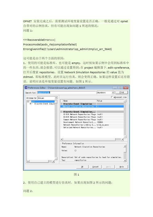
OPNET 安装完成之后，需要测试环境变量设置是否正确，一般是通过对opnet 自带对的示例仿真，但有可能出现如问题1所述的情况：问题1：<<<RecoverableError>>>|Processmodel(aodv_rte)compilationfailed|Errorsgiveninfile(C:\Users\Administrator\op_admin\tmp\cc_err_5640)这可能是由于两个方面的原因：1、使用的可能是标准库，也可能是empty，这时候如果示例中会用到标准库中的一些东西，就会报错，可以通过设置得到：在project编辑器下，edit->preference,打开后搜索repositories，设置Network Simulation Repositories的value值为stdmod，即标准模型，此时在运行仿真，则会变得正确，如果这样设置后还有错误，说明应该是环境变量设置有问题。

如图1所示。

图12、使用自己建立的模型进行仿真时，如果出现如图2所示的问题：问题2：<<< Program Abort >>>The set of models necessary for running the simulation is that all the 'repositories' attributes are (0), EV (-), MOD (NONE), PROC(sim_load_repos_load)图2这是因为我们用的模型库已经不是标准的模型库了，我们是自己创建的模型库，所以需要修改设置：就是将问题1设置的Network Simulation Repository值stdmod 删除，变回empty，如图3所示。

图3这样仿真就会正确了。

即使repository设置正确，有可能还会出现其它问题，以下几个是我遇到的：问题3：fatal error C1074: 'IDB' is illegal extension for PDB file（fatal error C1074: “IDB”是PDB 文件的非法扩展）这个问题主要是有兼容性问题造成的，我的系统时win7 32旗舰版，以及vs2010，打开opnet和vs程序的属性，在兼容性里设置如图4、如图5所示。

User's GuideSNVA037E–April2001–Revised April2013AN-1193LM3477Evaluation Board1IntroductionThe LM3477is a current mode,high-side N channel FET controller.It is most commonly used in buckconfigurations,as shown in Figure1.All the power conducting components of the circuit are external to the LM3477,so a large variety of inputs,outputs,and loads can be accommodated by the LM3477.The LM3477evaluation board comes ready to operate at the following conditions:4.5V≤V≤15VIN=3.3VVOUT0A≤I≤1.6AOUTThe circuit and BOM for this application are given in Figure1and Table1.Figure1.LM3477Buck ConverterAll trademarks are the property of their respective owners.1 SNVA037E–April2001–Revised April2013AN-1193LM3477Evaluation Board Submit Documentation FeedbackCopyright©2001–2013,Texas Instruments IncorporatedPerformance Table1.Bill of Materials(BOM)Component Value Part NumberC IN1120µF/20V594D127X0020R2C IN2No connectC OUT122µF/10V LMK432BJ226MM(Taiyo Yuden)C OUT222µF/10V LMK432BJ226MM(Taiyo Yuden)L10µH,3.8A DO3316P-103(Coilcraft)R C 1.8kΩCRCW08051821FRT1(Vitramon)C C112nF/50V VJ0805Y123KXAAT(Vitramon)C C2No connectQ15A,30V IRLMS2002(IRF)D100V,3A MBRS340T3(Motorola)R DR20ΩCRCW080520R0FRT1(Vitramon)R SL1kΩCRCW08051001FRT1(Vitramon)R FB116.2kΩCRCW08051622FRT1(Vitramon)R FB210.0kΩCRCW08051002FRT1(Vitramon)C FF470pF VJ0805Y471KXAAT(Vitramony)R SN0.03ΩWSL25120.03Ω±1%(Dale)2PerformanceThe following are some benchmark data taken from the circuit above on the LM3477evaluation board.This evaluation board can also be used to evaluate a buck regulator circuit optimized for a differentoperating point,or to evaluate a trade-off between cost and some performance parameter.For example,the conversion efficiency may be increased by using a lower RDS(ON)MOSFET,ripple voltage may belowered with lower ESR output capacitors,and the hysteretic threshold may be changed as a function ofthe RSN and RSLresistors.The conversion efficiency can be increased by using a lower RDS(ON)MOSFET,however it drops as inputvoltage increases.The efficiency reduces because of increased diode conduction time and increased switching losses.Switching losses are due to the Vds*Id transition losses and to the gate charge losses, both of which can be lowered by using a FET with low gate capacitance.At low duty cycles,where mostof the power loss in the FET is from the switching losses,trading off higher RDS(ON)for lower gatecapacitance will increase efficiency.Figure2.Efficiency vs Load VOUT=3.3V2AN-1193LM3477Evaluation Board SNVA037E–April2001–Revised April2013Submit Documentation FeedbackCopyright©2001–2013,Texas Instruments Incorporated Hysteretic ModeFigure 3.Efficiency vs V IN V OUT =3.3V,I OUT =2AFigure 5shows a bode plot of LM3477open loop frequency response using the external componentslisted in Table 1.(1)Magnitude =20dB/DecadeBandwidth =39.8kHz Phase =45°/Decade Phase Margin =41°Figure 4.Open Loop Frequency Response V IN =5V,V OUT =3.3V,I OUT =1.5A3Hysteretic ModeAs the load current is decreased,the LM3477will eventually enter a 'hysteretic'mode of operation.When the load current drops below the hysteretic mode threshold,the output voltage rises slightly.The overvoltage protection (OVP)comparator senses this rise and causes the power MOSFET to shut off.As the load pulls current out of the output capacitor,the output voltage drops until it hits the low threshold of the OVP comparator and the part begins switching again.This behavior results in a lower frequency,higher peak-to-peak output voltage ripple than with the normal pulse width modulation scheme.The magnitude of the output voltage ripple is determined by the OVP threshold levels,which are referred to the feedback voltage and are typically 1.25V to 1.31V.For more information,see the Electrical Characteristics table in the LM3477High Efficiency High-Side N-Channel Controller for Switching Regulator Data Sheet(SNVS141).In the case of a 3.3V output,this translates to a regulated output voltage between 3.27V and3.43V.The hysteretic mode threshold point is a function of R SN and R SL .Figure 5shows the Hysteretic Threshold vs.V IN for the LM3477evaluation board with and without R SL .3SNVA037E–April 2001–Revised April 2013AN-1193LM3477Evaluation Board Submit Documentation Feedback Copyright ©2001–2013,Texas Instruments IncorporatedIncreasing Current Limit Figure 5.I TH vs V IN4Increasing Current LimitThe R SL resistor offers flexibility in choosing the ramp of the slope compensation.Slope compensation affects the minimum inductance for stability (see the Slope Compensation section in the LM3477High Efficiency High-Side N-Channel Controller for Switching Regulator Data Sheet (SNVS141),but also helps determine the current limit and hysteretic threshold.As an example,R SL can be disconnected andreplaced by a 0ohm resistor so that no extra slope compensation is added to the current sense waveform to increase the current limit.A more conventional way to adjust the current limit is to change R SN .R SL is used here to change current limit for the sake of simplicity and to demonstrate the dependence of current limit to R SL .By changing R SL to 0ohm,the following conditions may be met:4.5V ≤V IN ≤15VV OUT =3.3V0A ≤I OUT ≤3AThe current limit is a weak function of slope compensation and a strong function of the sense resistor.By decreasing R SL ,slope compensation is decreased,and as a result the current limit increases.Thehysteretic mode threshold will also increase to about 1A (see Figure 5).Given below is a bode plot of LM3477open loop frequency response using the modified (R SL =0Ω)components to achieve higher output current capability.(1)Magnitude =20dB/DecadeBandwidth =55.3kHz Phase =45°/Decade Phase Margin =42°Figure 6.Open Loop Frequency Response V IN =5V,V OUT =3.3V,I OUT =3A4AN-1193LM3477Evaluation BoardSNVA037E–April 2001–Revised April 2013Submit Documentation FeedbackCopyright ©2001–2013,Texas Instruments Incorporated Layout Fundamentals 5Layout FundamentalsGood layout for DC-DC converters can be implemented by following a few simple design guidelines:1.Place the power components(catch diode,inductor,and filter capacitors)close together.Make thetraces between them short.e wide traces between the power components and for power connections to the DC-DC convertercircuit.3.Connect the ground pins of the input and output filter capacitors and catch diode as close as possibleusing generous component-side copper fill as a pseudo-ground plane.Then,connect this to theground-plane with several vias.4.Arrange the power components so that the switching current loops curl in the same direction.5.Route high-frequency power and ground return as direct continuous parallel paths.6.Separate noise sensitive traces,such as the voltage feedback path,from noisy traces associated withthe power components.7.Ensure a good low-impedance ground for the converter IC.8.Place the supporting components for the converter IC,such as compensation,frequency selection andcharge-pump components,as close to the converter IC as possible but away from noisy traces and the power components.Make their connections to the Converter IC and it's pseudo-ground plane as shortas possible.9.Place noise sensitive circuitry,such as radio-modem IF blocks,away from the DC-DC converter,CMOS digital blocks,and other noisy circuitry.Figure7.LM3477Evaluation Board PCB Layout(Top Side)5 SNVA037E–April2001–Revised April2013AN-1193LM3477Evaluation Board Submit Documentation FeedbackCopyright©2001–2013,Texas Instruments IncorporatedLayout Fundamentals Figure8.LM3477Evaluation Board PCB Layout(Bottom Side)6AN-1193LM3477Evaluation Board SNVA037E–April2001–Revised April2013Submit Documentation FeedbackCopyright©2001–2013,Texas Instruments IncorporatedIMPORTANT NOTICETexas Instruments Incorporated and its subsidiaries(TI)reserve the right to make corrections,enhancements,improvements and other changes to its semiconductor products and services per JESD46,latest issue,and to discontinue any product or service per JESD48,latest issue.Buyers should obtain the latest relevant information before placing orders and should verify that such information is current and complete.All semiconductor products(also referred to herein as“components”)are sold subject to TI’s terms and conditions of sale supplied at the time of order acknowledgment.TI warrants performance of its components to the specifications applicable at the time of sale,in accordance with the warranty in TI’s terms and conditions of sale of semiconductor products.Testing and other quality control techniques are used to the extent TI deems necessary to support this warranty.Except where mandated by applicable law,testing of all parameters of each component is not necessarily performed.TI assumes no liability for applications assistance or the design of Buyers’products.Buyers are responsible for their products and applications using TI components.To minimize the risks associated with Buyers’products and applications,Buyers should provide adequate design and operating safeguards.TI does not warrant or represent that any license,either express or implied,is granted under any patent right,copyright,mask work right,or other intellectual property right relating to any combination,machine,or process in which TI components or services are rmation published by TI regarding third-party products or services does not constitute a license to use such products or services or a warranty or endorsement e of such information may require a license from a third party under the patents or other intellectual property of the third party,or a license from TI under the patents or other intellectual property of TI.Reproduction of significant portions of TI information in TI data books or data sheets is permissible only if reproduction is without alteration and is accompanied by all associated warranties,conditions,limitations,and notices.TI is not responsible or liable for such altered rmation of third parties may be subject to additional restrictions.Resale of TI components or services with statements different from or beyond the parameters stated by TI for that component or service voids all express and any implied warranties for the associated TI component or service and is an unfair and deceptive business practice. TI is not responsible or liable for any such statements.Buyer acknowledges and agrees that it is solely responsible for compliance with all legal,regulatory and safety-related requirements concerning its products,and any use of TI components in its applications,notwithstanding any applications-related information or support that may be provided by TI.Buyer represents and agrees that it has all the necessary expertise to create and implement safeguards which anticipate dangerous consequences of failures,monitor failures and their consequences,lessen the likelihood of failures that might cause harm and take appropriate remedial actions.Buyer will fully indemnify TI and its representatives against any damages arising out of the use of any TI components in safety-critical applications.In some cases,TI components may be promoted specifically to facilitate safety-related applications.With such components,TI’s goal is to help enable customers to design and create their own end-product solutions that meet applicable functional safety standards and requirements.Nonetheless,such components are subject to these terms.No TI components are authorized for use in FDA Class III(or similar life-critical medical equipment)unless authorized officers of the parties have executed a special agreement specifically governing such use.Only those TI components which TI has specifically designated as military grade or“enhanced plastic”are designed and intended for use in military/aerospace applications or environments.Buyer acknowledges and agrees that any military or aerospace use of TI components which have not been so designated is solely at the Buyer's risk,and that Buyer is solely responsible for compliance with all legal and regulatory requirements in connection with such use.TI has specifically designated certain components as meeting ISO/TS16949requirements,mainly for automotive use.In any case of use of non-designated products,TI will not be responsible for any failure to meet ISO/TS16949.Products ApplicationsAudio /audio Automotive and Transportation /automotiveAmplifiers Communications and Telecom /communicationsData Converters Computers and Peripherals /computersDLP®Products Consumer Electronics /consumer-appsDSP Energy and Lighting /energyClocks and Timers /clocks Industrial /industrialInterface Medical /medicalLogic Security /securityPower Mgmt Space,Avionics and Defense /space-avionics-defense Microcontrollers Video and Imaging /videoRFID OMAP Applications Processors /omap TI E2E Community Wireless Connectivity /wirelessconnectivityMailing Address:Texas Instruments,Post Office Box655303,Dallas,Texas75265Copyright©2013,Texas Instruments Incorporated。

MV2F错误代码中⽂解释MSH错误信息⼀览表错误代码显⽰信息原因处理⽅法EQ0001 Head inclination measurement impossible 进⾏取消设定测量时,吸嘴1设定成NGEQ0025 Y--axis origin 通过副操作盘旋转主轴时,Y轴在原点①按亮副操作盘键②⽤MANUAL JOG 功能,将Y轴移出原点EQ0031 Cam axis origin detection error A ①凸轮轴⽪带坏①更换⽪带②凸轮轴原点检测器失效或②更换或清洗检测器有脏物附着③调整槽盘位置③原点检测⽤槽盘错位EQ0032 Cam axis origin detection error B ①凸轮轴⽪带坏①更换⽪带②凸轮轴原点检测器失效或②更换或清洗检测器有脏物附着③调整槽盘位置③原点检测⽤槽盘错位EQ0046 Nozzle origin check sensor error 吸嘴原点没有到位①检查原点传感器位置②检查接⼝③调整传感器灵敏度④⽤⼿将吸嘴转⾄原点EQ0053 S nozzle suction bad warning ⼩吸嘴吸着不良报警并被⾃动跳跃①清洗吸嘴更换过滤垫②检查吸嘴安装情况③重新测定吸嘴⾼度和中⼼④更换吸嘴⑤检查部品库参数设置⑥检查厚度传感器是否被异物遮盖⑦检查真空泵是否开启⑧检查料架供料情况EQ0054 M nozzle suction bad warning 中号吸嘴吸着不良报警并被⾃动跳跃①清洗吸嘴更换过滤垫②检查吸嘴安装情况③重新测定吸嘴⾼度和中⼼④更换吸嘴⑤检查部品库参数设置⑥检查厚度传感器是否被异物遮盖⑦检查真空泵是否开启⑧检查料架供料情况EQ0055 L nozzle suction bad warning ⼤号吸嘴吸着不良报警并被⾃动跳跃①清洗吸嘴更换过滤垫②检查吸嘴安装情况③重新测定吸嘴⾼度和中⼼④更换吸嘴⑤检查部品库参数设置⑥检查厚度传感器是否被异物遮盖⑦检查真空泵是否开启⑧检查料架供料情况EQ0056 S nozzle recognition bad warning ⼩号吸嘴识别不良报警并被⾃动跳跃①清洗吸嘴更换过滤垫②检查吸嘴安装情况③重新测定吸嘴⾼度和中⼼④更换吸嘴⑤检查部品库参数设置⑥检查厚度传感器是否被异物遮盖⑦检查真空泵是否开启⑧检查料架供料情况EQ0057 M nozzle recognition bad warning 中号吸嘴识别不良报警并被⾃动跳跃①清洗吸嘴更换过滤垫②检查吸嘴安装情况③重新测定吸嘴⾼度和中⼼④更换吸嘴⑤检查部品库参数设置⑥检查厚度传感器是否被异物遮盖⑦检查真空泵是否开启⑧检查料架供料情况EQ0058 L nozzle recognition bad warning ⼤号吸嘴识别不良报警并被⾃动跳跃①清洗吸嘴更换过滤垫②检查吸嘴安装情况③重新测定吸嘴⾼度和中⼼④更换吸嘴⑤检查部品库参数设置⑥检查厚度传感器是否被异物遮盖⑦检查真空泵是否开启⑧检查料架供料情况EQ0059 S nozzle switch bad warning ⼩号吸嘴切换不良报警并被⾃动跳跃①清洗吸嘴更换过滤垫②检查吸嘴安装情况③重新测定吸嘴⾼度和中⼼④更换吸嘴⑤检查部品库参数设置⑥检查厚度传感器是否被异物遮盖⑦检查真空泵是否开启⑧检查料架供料情况EQ0060 M nozzle switch bad warning 中号吸嘴切换不良报警并被⾃动跳跃①清洗吸嘴更换过滤垫②检查吸嘴安装情况③重新测定吸嘴⾼度和中⼼④更换吸嘴⑤检查部品库参数设置⑥检查厚度传感器是否被异物遮盖⑦检查真空泵是否开启⑧检查料架供料情况EQ0061 L nozzle switch bad warning ⼤号吸嘴切换不良报警并被⾃动跳跃①清洗吸嘴更换过滤垫②检查吸嘴安装情况③重新测定吸嘴⾼度和中⼼④更换吸嘴⑤检查部品库参数设置⑥检查厚度传感器是否被异物遮盖⑦检查真空泵是否开启⑧检查料架供料情况EQ0062 No s nozzle ready for suction 所有⼩吸嘴因吸着、识别或切换不良⽽全部跳跃①清洗吸嘴更换过滤垫②检查吸嘴安装情况③重新测定吸嘴⾼度和中⼼④更换吸嘴⑤检查部品库参数设置⑥检查厚度传感器是否被异物遮盖⑦检查真空泵是否开启⑧检查料架供料情况EQ0063 No m nozzle ready for suction 所有中吸嘴因吸着、识别或切换不良⽽全部跳跃①清洗吸嘴更换过滤垫②检查吸嘴安装情况③重新测定吸嘴⾼度和中⼼④更换吸嘴⑤检查部品库参数设置⑥检查厚度传感器是否被异物遮盖⑦检查真空泵是否开启⑧检查料架供料情况EQ0064 No l nozzle ready for suction 所有⼤吸嘴因吸着、识别或切换不良⽽全部跳跃①清洗吸嘴更换过滤垫②检查吸嘴安装情况③重新测定吸嘴⾼度和中⼼④更换吸嘴⑤检查部品库参数设置⑥检查厚度传感器是否被异物遮盖⑦检查真空泵是否开启⑧检查料架供料情况EQ0112 Parts exchange incompleteness 未换料按开始键将后部按亮HC0001 Handle interlock ①主轴摇动⼿轮没有拔出来①拔出⼿轮②⼿轮位置传感器失效或需②更换或重新调整传感器要调整③检查传感器与P-922M的连接情况HC0015 Head axis brake ON 主轴旋转时,break开关仍在ON位置置于OFFHC0016 Head axis servo motor OFF 主轴servo开关处于OFF位置置于ONHC0017 Head-axis origin OFF ①cycle timer ch1 信号没有的①⼿动将主轴回到原点100-200情况下,操作者试图移动某轴②检查cycle timer 设置情况② cycle timer 设置错误HC0024 Feed return detection error ① cycle timer 3350-1600时检①检查传感器检测设定情况测复位时, ②重新调整系统传感器灯并没有亮③更换或调整复位②系统坏传感器③复位传感④检查传感器与光模块的连接情况器损坏或需要调整HC0028 Head number detection error ①传感器检测内容与先前设①调整或更换吸嘴单元号码，检测定内容不⼀致传感器②传感器检测值不在1-16范②检查传感器与光模块连接情况围内③吸嘴单元头号码检测传感器失效、调整不良或连接不好HC0029 Nozzle number detection error ①传感器检测内容不正常①交换或调整第⼀个传感器②传感器检测内容不是1-3 ②检查⼤、中、⼩吸嘴安装情况是③不良元件检测位置前⾯的否滑动顺畅⼤中⼩号吸嘴检测传感器③检查第⼀个 sensor (传感器)与坏了、调整不良或接线不 P-922M 的连接情况良HC0033 Nozzle return detectionerror 传感器坏了或调整不当更换或调整 sensorHC0036 Safety detection error 安全传感器1或2开始⽣效HC0037 activated at θ axis starting θ轴起动过程不正常检查 cycle timer ⾓度HC0041 Sc movement impossible ①Sc程序Rom控制器坏①关机开机⼀次②Sc基板坏②更换Sc电路板HC0042 Suction miss ( no suction ) ①在修正值之内元件仍吸着①重新设定次数不良,最后⼀次不良为未 (最多5次)吸着②将料架安放准确②料架搁放位置不对③清洗、更换 nozzle③吸嘴坏或被堵塞④检查部品厚度值设定④部品数据库厚度值设定不对⑤厚度传感器测量错误HC0043 Suction miss standing ①在修正值之内元件仍吸着①重新设定次数不良,最后⼀次不良为⽴ (最多5次)起②将料架安放准确②料架搁放位置不对③清洗、更换 nozzle③吸嘴坏或被堵塞④检查部品厚度值设定④部品数据库厚度值设定不对⑤厚度传感器测量错误HC0051 Thickness sensor error ①厚度传感器不在⾃动状态①打开②输⼊/输出光电模块坏或连接②更换光电模块不好③检查传感器与控制部分接线情况③电源未开④开机、关机⼀次④厚度传感器控制部分坏⑤更换厚度传感器⑤未进⾏设置HC0052 Thickness sensor time up ①厚度传感器在极限⾓度3370 ① ON仍未完成测量②更换光电模块②传感器在⼿动状态③检查厚度传感器与控制部分接线③传感器坏④检查传感器与光电模块的接线⑤更换 SENSOR⑥检查是否灯已亮HC0054 Thickness sensor data abnormal 厚度传感器数据不正常①检查接线情况②检查部品厚度数据HC0056 Cassette seating detection error ①料架安放不平检查料架安放情况②料架压板传感器坏HC0058 Cassette setting mistake 1 miss (1) ①料架安放错误①安放正确料架②料架设定传感器坏或调整不②更换或调整 sensor良③检查传感器与光电模块连接情况③料架 shutter 不平HC0059 Cassette setting mistake 2 miss (2) ①料架安放错误①安放正确料架②料架设定传感器坏或调整不②更换或调整 sensor良③检查传感器与光电模块连接情况③料架 shutter 不平HC0061 Left safety detection error 左侧安全门有⼈HC0062 Right safety detection error ①右边Z轴料未换完,右边安全①调整或更换传感器传感器熄灭②检查安全传感器与光电模块的连②右边安全传感器坏或需要调接情况整③检查后部Z轴是有⼈进⼊或有异③有⼈或东西进⼊安全门轨道物阻隔区域内HC0063 Center safety detection error ①中间Z轴料未换完,中间安全①调整或更换传感器传感器熄灭②检查安全传感器与光电模块的连②中间安全传感器坏或需要调接情况整③检查后部Z轴是有⼈进⼊或有异③有⼈或东西进⼊安全门轨道物阻隔区域内HC0064 Right cassette floating detection error 右边Z轴料架浮起①检查料架安放情况②检查传感器是否已坏HC0065 Left cassette floating detection error 左边Z轴料架浮起①检查料架安放情况②检查传感器是否已坏HC0066 Laser radiatior ①开关ON②开关坏③开关与光电模块连接不当HC0069 Left laser detection error 左侧料架压紧、传感器坏更换 sensorHC0070 Right laser detection error 右侧料架压紧、传感器坏更换 sensorHC0073 Zl - axis standby detection error ①Zl换料时等待传感器灭①检查是否 OFF移动了②Zl换料时，Zl被移动 Z轴③Zl等待传感器坏或需要调整②确认换料时Zl移到等待位置时，④ OFF后移动Zl轴等待 sensor 灯亮③调整或更换Zl待机传感器④检查传感器与光电模块的连接情况⑤ RESETHC0074 ZR - axis standby detection error ①ZR换料时等待传感器灭①检查是否 OFF移动了②ZR换料时，Zl被移动 Z轴③ZR等待传感器坏或需要调整②确认换料时ZR移到等待位置时，④ OFF后移动ZR轴等待 sensor 灯亮③调整或更换ZR待机传感器④检查传感器与光电模块的连接情况⑤ RESETHC0077 Zl - axis other error ZL轴其它错误 mmc unit error HC0078 ZR - axis other error ZR轴其它错误 mmc unit error HC0079 ZL - axis ready error ZL处于准备状态时操作者试图开始 OFF绿灯亮后startHC0080 ZR - axis ready error ZR处于准备状态时操作者试图开始 OFF绿灯亮后startHC0082 ZL - ZR table ready ZL ZR 因⽆料⽽全部处于准备状态 OFF绿灯亮后startHC0083 Large component pickup error ⼤元件吸嘴未吸起来将元件从料带中拿出来HC0084 Waste box setting error ①纸屑箱安放不良①将纸屑箱安装好②纸屑箱检测传感器坏②更换传感器HC0085 Nozzle error 部品厚度检测值为0 吸嘴折MC0001 air down ①未供⽓调整⽓压②⽓压低于4kg/cm2MC0002 Thermal trip ①热保护信号断①将主控制板热保护开关置于ON②200V电压突然切断②将纸屑箱热保护复位③真空泵或料屑箱热保护继电③检查真空泵转动⽅向器跳闸④检查纸屑箱泵转动⽅向④料屑箱4P接⼝断⑤检查纸屑箱是否已被堵塞⑥检查保险丝⑦检查4P接⼝连接情况MC0003 All axes servo motorOFF OFF ONMC0004 Emergency stop 开关被压下①开关松开②检查接线MC0005 Safety stop 开后⾃然出现⼀次或n次MC0006 1 block stop ①前盖开 OFF②前盖关 ON③轨道宽度调节⼿柄⽤完后未放回原位MC0007 cycle timer sequence error ⼿柄反向转动 H axis 回原点100-200MC0008 cycle timer abnormal 失效关机检查及接线情况MC0100 Planned production number fineshed ⽣产计划已完⼜重新设定或选择⽣产计划数 .MC0101 Planned production number finished 半⾃动吸着已完⼜退出现画⾯MC0203 ZL parts exhaust ①连续吸着错误数超过设定值①更换新料②Z轴⽆料②重新设置部品数据③料架位置不对③清洗更换 nozzle④吸嘴脏或坏⑤部品数据设置不对⑥厚度传感器测量错误MC0204 ZR parts exhanst ①连续吸着错误数超过设定值①更换新料②Z轴⽆料②重新设置部品数据③料架位置不对③清洗更换 nozzle④吸嘴脏或坏⑤部品数据设置不对⑥厚度传感器测量错误MC0305 Recognition error 识别错误①检查部品库元件长宽尺⼨②检查发光管发光情况MC0400 Parts exhaust warning 某料快⽤完备料MC0500 Operation error 操作失误①开始时跳过半⾃动②检测吸嘴中⼼照相机初期设定元件进⾏部品库识别时未回原点③⼤中⼩吸嘴设定不对④吸嘴全部NG时 StartMC0502 Operation mode switch interlock error 操作者切换运转状态(Auto semi manual)时机不对进⾏输了开始步,全⾃动时不能切换MC0503 Stop mode switch interlock error 操作者⾮法未设定就StopMC0504 On-line mode switch interlock error 操作者⾮法MC0508 Origin return interlock error 操作者⾮法退出状态MC0510 Mount start interlock error 操作者⾮法下列情况不能开始①数据编辑②部品识别③输⼊起始步画⾯④X-Y teaching 功能⑤半⾃动吸着MC0511 Origin return incompleness error 开机后未回原点MC0513 Head-axis restart impossible 控制器内⼀个NC线路板坏更换NC线路板MC0514 No P.C.B on the XY table XY⼯作上没有基板试图全⾃动开始①装载基板②调整基板存在传感器③检查基板存在传感器与光电模块联接情况MC0522 Unmounted block 由于机器故障、关掉电源等原因基板尚未贴完的步数①START 继续吸着②停⽌吸着，将按灭③吸着后检查⼀下基板吸着是否正确MC0523 Mounting side block no cassette NC程序与配列程序搭配不当①重新选择NC程序、配列程序②更改数据MC0600 No mounting command ①未选程序①选择程序②所选程序步骤为0 ②更改程序③执⾏程序不存在③检查程序跳步是否正确④执⾏步数在NC程序不存在MC0603 No Z alteration component ①Z轴数值不对①重新设置 multi--origin 补偿值②主Z轴设置不对②重新设置 Z alteration③主Z轴设置跨越ZL、ZR ③重新设置 master ZMC0604 Start block designation error 起始步设定不对不能开始于第⼀步因第⼀步为基板识别MC0605 No program setting error ①NC程序不对①Z轴联接使⽤时Z轴数不超过150②步重复命令和块重复命令混②Z轴交换或准备状态时Z轴数不超合使⽤过75MC0607 M000 command in NC data abnormal NC data 不对MC0608 M100 command in NC data abnormal NC data 不对MC0610 M200 command in NC data abnormal NC data 不对MC0611 M command in NC data abnormal NC data 不对MC0613 NC program Pcb recognition command setting error 基板识别放在了吸着步数中间MC0614 Bad mark command in NC data abnormal 不良基板识别放在了吸着步数中间MC0615 Recognition command in NC data abnormal MMC或MMI电路电池⽤完后重新从软盘输⼊程序MC0616 Array program edit error 配列程序中有些数值没有输⼊MC0617 Array program setting error 配列程序数据不对重新编辑MC0620 Parts data abnormal ①部品库某些数值不对重新编辑②部品库某些数值未输MC0621 Parts data setting error ①某些数值在MSHⅡ上不能重新编辑使⽤②速度超过8,吸嘴超过3.③压料次数部品厚度识别数据设定为0MC0624 Mark data setting error ①未做Mark识别②Mark库代码为0MC0628 Multi orgin data error Z轴起始原点超过范围①Z 轴联接超过150②Z轴交换或准备超过75③Z轴超过程序Z数MC0631 S&R block number over 步重复或块重复步数超过200 REEDITMC0900 Parts camera scale not set 照相机像素未设定 SCALE 重新设定MC0908 Parts replacement warning (light for board) 发光管使⽤时间超过设定值更换发光管然后重新设定报警时间MC1000 X-axis plus soft limit 下列数值设定不对使机床超过X⽅向正极限①检查机床初期设定X⽅向机器原点是否正确●机器原点②进⼊程序编辑状态,检查X⽅向程●程序原点序原点是否正确●照相机相素③进⼊机床初期设定识别数据基础●照相机位置补偿值值,检查照相机像素和位置补偿值是否正确MC1001 X-axis minus soft limit 下列数值设定不对使机床超过X ⽅向负极限①检查机床初期设定X⽅向机器原点是否正确●机器原点②进⼊程序编辑状态,检查X⽅向程●程序原点序原点是否正确●照相机相素③进⼊机床初期设定识别数据基础●照相机位置补偿值值,检查照相机像素和位置补偿值是否正确MC1002 Y-axis plus soft limit 下列数值设定不对使机床超过Y ⽅向正极限①检查机床初期设定Y⽅向机器原点是否正确●机器原点②进⼊程序编辑状态,检查Y⽅向程●程序原点序原点是否正确●照相机相素③进⼊机床初期设定识别数据基础●照相机位置补偿值值,检查照相机像素和位置补偿值是否正确MC1003 Y-axis minus soft limit 下列数值设定不对使机床超过Y ⽅向负极限①检查机床初期设定Y⽅向机器原点是否正确●机器原点②进⼊程序编辑状态,检查Y⽅向程●程序原点序原点是否正确●照相机相素③进⼊机床初期设定识别数据基础●照相机位置补偿值值,检查照相机像素和位置补偿值是否正确MC1004 ZL-axis plus soft limit ZL轴设定值不对超过正极限检查初期设定值ZL数据是否正确MC1005 ZL-axis minus soft limit ZL轴设定值不对超过负极限检查初期设定值ZL数据是否正确MC1006 ZR-axis plus soft limit 下列数值设定不对造成ZR超过正极限检查机床初期设定Z轴原点补偿及Z轴间距是否正确●Z轴原点补偿值●Z轴间距MC1007 ZR-axis minus soft limit 下列数值设定不对造成ZR超过负极限检查机床初期设定Z轴原点补偿及Z轴间距是否正确●Z轴原点补偿值●Z轴间距MC1102 ZL-axis interlock error atstart ① 3120-1580 Z轴移动时Z互锁信号关闭①检查设定情况②调整辅助进给单元上极限传感器②辅助进给单元上极限传感器需要调整或未联接③检查辅助进给单元上极限传感器与光电模块的联接情况③辅助进给马达原点传感器需要调整或连线已断④调整辅助进给马达原点传感器⑤检查辅助进给马达与江电模块联接情况④Z轴处于准备状态时,伺服锁定被打开.⑥重新操作MC1103 ZR-axis interlock error atstart ① 3200-1600 Z轴移动时Z互锁信号关闭①检查设定情况②调整辅助进给单元上极限传感器②辅助进给单元上极限传感器需要调整或未联接③检查辅助进给单元上极限传感器与光电模块的联接情况③辅助进给马达原点传感器需要调整或连线已断④调整辅助进给马达原点传感器⑤检查辅助进给马达与江电模块联接情况④Z轴处于准备状态时,伺服锁定被打开.⑥重新操作MC9000 P783 fan motor alarm P783控制器冷却风扇坏或风扇电线断MC9001 P783 overheat P783控制器内温度超过500 更换冷却风扇MC9010 NC card error (1) ①NC板被接通后没反应关掉电源检查控制器内NC板②电源打开或后出现⼀个初期错误MC9011 NC card error (2) 信号传输不可能时命令从MMC板到达NC1板或NC2板关掉电源检查控制器内NC1板和NC2板MC9012 NC card error (3) 控制器内NC板接触不良或已坏关掉电源检查控制器内NC板MC9015 PM card error (1) 信号传输不可能时命令从MMC板到达PM 板关掉电源检查控制器内PM板MC9016 PM card error (2) 控制器内PM板接触不良或已坏关掉电源检查控制器内PM板MC9020 SC card error (1) 控制器内SC板失效或已坏关掉电源检查控制器内SC板MC9021 SC card error (2) 信号传输不可能时命令从MMC板到达SC 板关掉电源检查控制器内SC板MC9022 SC card error (3) 控制器内SC板失效或已坏关掉电源检查控制器内SC板MC9023 SC card error (4) 控制器内SC板接触不良或坏关掉电源检查控制器内SC板MC9025 RE card error (1) 控制器内RC板失效或已坏关掉电源检查控制器内RC板MC9026 RE card error (2) 信号传输不可能时命令从MMC板到达RC 板关掉电源检查控制器内RC板MC9027 RE card error (3) 控制器内RC板接触不良或坏关掉电源检查控制器内RC板MC9030 MMI card error (1) 控制器内MMI板失效或已坏关掉电源检查控制器内MMI板MC9031 MMI card error (2) 信号传输不可能时命令从MMC板到达MMI板关掉电源检查控制器内MMI板MC9032 MMI card error (3) 控制器内MMI板接触不良或坏关掉电源检查控制器内MMI板NC0100 X-axis plus limit ①X轴移动超过X轴正极限①调整X轴正极限传感器灵敏度及位②X轴正极限传感器位置设置置不对②检查X轴正极限传感器与光电模块③正极限传感器坏联接情况NC0101 X-axis minus limit ①X轴移动超过X轴负极限①调整X轴负极限传感器灵敏度及位②X轴负极限传感器位置设置置不对②检查X轴负极限传感器与光电模块③负极限传感器坏联接情况NC0102 X-axis deviation counter overflow ①伺服马达开关处于OFF 关掉电源调整马达驱动器②X轴⽅向过载(加速过快)③X轴驱动器(GAIN STB)需要调整④X轴移动过程中马达脱离啮合⑤X轴丝杠脏造成X轴移动不了NC0103 X-axis driver alarm ①X轴马达过流(OC) ①关掉电源调整X轴马达驱动器②X轴马达电源被关②检查X轴驱动器电源③移动中驱动器信号断③检查X轴安全极限传感器是否0FF④回原点时互锁信号断NC0104 X-axis time up ①X轴定位超过5秒关掉电源调整X 轴驱动器②X轴速度设定错误③原点回归超过20秒④H轴或其它轴需要调整⑤控制器内有错误NC0105 X-axis interlock during moverment ①X轴运转过程中 33频道互锁信号断①关掉电源检查⾓度设定及接线情况②H轴或其它轴需要调整②调整X轴驱动器③X轴驱动器需要调整④设定不良⑤XY开始信号被切断NC0106 X-axis movement impossible ①X轴驱动器电源未开①检查X轴驱动器电源②X轴驱动器与控制器接线不良②关掉总电源检查X轴驱动器与控制③X轴移动时马达准备信号断器的接线情况NC0107 X-axis origin detection error ①X轴原点传感器已坏①调整X轴原点传感器②由于接线不良致使传感器检②检查X轴原点传感受器与光电模块测不到原点的联接情况③检查X轴原点减速传感器与光电模块的接线情况NC0112 X-axis error (others) X轴由于任意错误⽽突然停⽌通常屏幕上会显⽰⼀些其它错误根据错误显⽰内容检查错误原因并及时处理NC0200 Y-axis plus limit ①Y轴移动超过Y轴正极限①调整Y轴正极限传感器灵敏度及位②Y轴正极限传感器位置设置置不对②检查Y轴正极限传感器与光电模块③正极限传感器坏联接情况NC0201 Y-axis minus limit ①Y轴移动超过Y轴负极限①调整Y轴负极限传感器灵敏度及位②Y轴负极限传感器位置设置置不对②检查Y轴负极限传感器与光电模块③负极限传感器坏联接情况NC0202 Y-axis deviation counter overflow ①伺服马达开关处于OFF 关掉电源调整马达驱动器②Y轴⽅向过载(加速过快)③Y轴驱动器(GAIN STB)需要调整④Y轴移动过程中马达脱离啮合⑤Y轴丝杠脏造成Y轴移动不了NC0203 Y-axis driver alarm ①Y轴马达过流(OC) ①关掉电源调整Y轴马达驱动器②Y轴马达电源被关②检查Y轴驱动器电源③移动中驱动器信号断③检查Y轴安全极限传感器是否0FF④回原点时互锁信号断NC0204 Y-axis time up ①Y轴定位超过5秒关掉电源调整Y 轴驱动器②Y轴速度设定错误③原点回归超过20秒④H轴或其它轴需要调整⑤控制器内有错误NC0205 Y-axis interlock during moverment ①Y轴运转过程中 33频道互锁信号断①关掉电源检查⾓度设定及接线情况②H轴或其它轴需要调整②调整Y轴驱动器③Y轴驱动器需要调整④设定不良⑤XY开始信号被切断NC0206 Y-axis movement impossible ①Y轴驱动器电源未开①检查Y轴驱动器电源②Y轴驱动器与控制器接线不良②关掉总电源检查Y轴驱动器与控制③Y轴移动时马达准备信号断器的接线情况NC0207 Y-axis origin detection error ①Y轴原点传感器已坏①调整Y轴原点传感器②由于接线不良致使传感器检②检查Y轴原点传感受器与光电模块测不到原点的联接情况③检查Y轴原点减速传感器与光电模块的接线情况NC0212 Y-axis error (others) Y轴由于任意错误⽽突然停⽌通常屏幕上会显⽰⼀些其它错误根据错误显⽰内容检查错误原因并及时处理NC0300 Z-axis plus limit ①Z轴移动超过Z轴正极限①调整Z轴正极限传感器灵敏度及位②Z轴正极限传感器位置设置置不对②检查Z轴正极限传感器与光电模块③正极限传感器坏联接情况NC0301 Z-axis minus limit ①Z轴移动超过Z轴负极限①调整Z轴负极限传感器灵敏度及位②Z轴负极限传感器位置设置置不对②检查Z轴负极限传感器与光电模块③负极限传感器坏联接情况NC0302 Z-axis deviation counter overflow ①伺服马达开关处于OFF 关掉电源调整马达驱动器②Z轴⽅向过载(加速过快)③Z轴驱动器(GAIN STB)需要调整④Z轴移动过程中马达脱离啮合⑤Z轴丝杠脏造成Z轴移动不了NC0303 Z-axis driver alarm ①Z轴马达过流(OC) ①关掉电源调整Z轴马达驱动器②Z轴马达电源被关②检查Z轴驱动器电源③移动中驱动器信号断③检查Z轴安全极限传感器是否0FF④回原点时互锁信号断NC0304 Z-axis time up ①Z轴定位超过5秒关掉电源调整Z 轴驱动器②Z轴速度设定错误③原点回归超过20秒④H轴或其它轴需要调整⑤控制器内有错误NC0305 Z-axis interlock during moverment ①Z轴运转过程中 33频道互锁信号断①关掉电源检查⾓度设定及接线情况②H轴或其它轴需要调整②调整Z轴驱动器③Z轴驱动器需要调整④设定不良⑤XY开始信号被切断NC0306 Z-axis movement impossible ①Z轴驱动器电源未开①检查Z轴驱动器电源②Z轴驱动器与控制器接线不良②关掉总电源检查Z轴驱动器与控制③Z轴移动时马达准备信号断器的接线情况NC0307 Z-axis origin detection error ①Z轴原点传感器已坏①调整Z轴原点传感器②由于接线不良致使传感器检②检查Z轴原点传感受器与光电模块测不到原点的联接情况③调整Z轴缝隙传感器④检查Z轴原点减速传感器与光电模块的接线情况NC0312 Z-axis error (others) Z轴由于任意错误⽽突然停⽌通常屏幕上会显⽰⼀些其它错误根据错误显⽰内容检查错误原因并及时处理NC0402 θ1-axis deviation counter overflow ①伺服马达开关处于OFF 关掉电源调整马达驱动器②θ1轴⽅向过载(加速过快)③θ1轴驱动器(GAIN STB)需要调整④θ1轴移动过程中马达脱离啮合⑤θ1轴丝杠脏造成其不能移动NC0403 θ1-axis driver alarm ①θ1轴马达过流(OC) ①关掉电源调整θ1轴马达驱动器②θ1轴马达电源被关②检查θ1轴驱动器电源③移动中驱动器信号断③检查θ1轴安全极限传感器是否0FF④回原点时互锁信号断NC0404 θ1-axis time up ①θ1轴定位超过5秒关掉电源调整θ1轴驱动器②θ1轴速度设定错误③原点回归超过20秒④H轴或其它轴需要调整⑤控制器内有错误NC0405 θ1-axis interlock during moverment ①θ1轴运转过程中 33频道互锁信号断①关掉电源检查⾓度设定及接线情况②H轴或其它轴需要调整②调整θ1轴驱动器③θ1轴驱动器需要调整④设定不良。

The brand new concept of EMI probesApplication NoteIndex1.Simplify the complicated EMC measurement and debugging! (3)2.The Advantages of GKT-008 EMI Near Field Probe Set (3)3.GKT-008 EMI Near Field Probe Set (3)4.Normal EMI Test on Lab (4)5.Swiftly Simplify Complicated EMI Measurement and Debugging (5)6.New Generation Probes to Accurately Find Radiation Source (6)7.Problems Facing General Near Field Probes (9)8.Practical Cases (12)rmation of Product Ordering (14)Simplify the complicated EMC measurement and debugging!As a result of faster and faster consumer electronics products, the frequency of conducting EMI tests becomes higher and higher. The continuous integration of parts in electronics products and the number of parts involved are also swiftly increasing. Besides, the demand of EMI regulations from countries and regions is getting stricter than ever. But the life cycle of electronics products is getting shorter and shorter. Hence, in order to effectively and quickly solve EMI issues at the development stage and reduce the number of times products going to the lab, a simple and easy set of tool to quickly help engineers find EMI source to greatly expedite products’ time to market is essentially required.GW Instek launches the new patent GKT-008 electromagnetic field probes, which are small and highly sensitive. GKT-008 probes can directly sense EMI signal energy unlike conventional near field probes which require using electric field probes and magnetic field probes to measure electric field and magnetic field separately. Users can save costs from product development cycles and the lab that is conducive to expedite time for product verification and product launch.The Advantages of GKT-008 EMI Near Field Probe SetThe conventional magnetic field probes are hollow loop probes. When the magneticfield is perpendicular to probe’s loop surface, the maximum measurement value canbe obtained. The maximum magnetic field value can only be measured by rotatingpr obe’s direction.GKT-008 EMI near field probe features high spatial resolution and sensitivity withoutrotating probe’s direction to measure the maximum magnetic field value so as toidentify the main radiation signal source. This probe set aims at carrying out pre-testand debug of EMI field scanner so as to effectively obtain EMI source, segmentedfrequency strength of EMI source, etc. that provides key indicators for resolving EMCissues. By this probe set, users can formulate solutions to amend failed products.GKT-008 EMI Near Field Probe SetGKT-008 EMI Near Field Probe Set comprises four probes, including PR-01, PR-02, ANT-04, and ANT-05. The antenna factors of these four probes are built in the EMC Pretest function of GSP-9300 spectrum analyzer.- ANT-04 and ANT-05 are EMI field sensor, which can maximally sustainCAT I 50Vdc. ANT-04 and ANT-05 magnetic field probes will collocatewith ADB-008 DC block to avoid damaging spectrum analyzer and theRF input terminal of DUT receiver.- PR-01 is an AC voltage probe, which can maximally sustain CAT II,300VAC. PR-01 AC voltage probe will collocate with GPL-5010 transientlimiter and BNC (M) to SMA (F) adaptor to avoid damaging spectrumanalyzer and the RF input terminal of DUT receiver.- PR-02 is an EMI source contact probe, which can maximally sustain CATI 50V DC. PR-02 electric field probe will collocate with ADB-008 DCblock to avoid damaging spectrum analyzer and the RF input terminal ofDUT receiver.Normal EMI Test on LabFor a formal EMI certification test, in either an EMI chamber or an open fieldsite, the receiving antenna will pick up the emissions with in a distance of 8 or10 meters. This means the emissions may come from anywhere within the DUT.The antenna will receive them all the emissions, they can come from the top,bottom, right or left hand side.EMI test at Open Area TestSiteEMI Test in Anechoic ChamberIn Figure, the DUT is placed on a rotatable table, the receiving antenna islocated 10 meters from the DUT, and its stature is adjustable. The antennaoutput is connected to a spectrum analyzer which is located in a shielded room.A perfect Ground is needed to ensure an isolated environment. During themeasurement, the table will rotate 360 degrees, so that the antenna canreceive the Omni directional emissions. The antenna is also vertically adjustableto catch the upward emissions.However, the EMI testing results can not distinguish where on the DUT theemissions were generated. When the emissions are too strong and fail to passregulations, the source needs to be suppressed and thus have to be identifiedfirst. The near field probe is used to find the source of emissions on the DUT.Swiftly Simplify Complicated EMI Measurement and DebuggingGeneral issues of near field measurementsUsually, engineers will use near field probes to conduct EMI tests for circuit verification. However, they will encounter same problems when carrying out the test. • Probes can not quickly identify which circuit the radiation sourcecomes from. • Engineers have to use magnetic field probes and electric field probesseparately for measurements and they have to use their experience to find the signal source. • The angle or position of magnetic field probes will complicate themeasurements.The main reason behind these problems is that near field probes in the past are distinguished by magnetic field probe and electric field probe. In fact, engineers are concerned about how signal ’s energy emits. Hence, it is very important to correctly and quickly find the major energy emission source.- Probe sizeNormally, larger near field probes are used to sense electromagnetic field. But they can not easily identify the source of radiation. On the other hand,- The difference between electricfield probe and magnetic field probeIt is very difficult to judge the real signal source by waveforms obtained from measurements of electric field probes and magnetic field probes separately. Because these waveforms are very different from each other.- The angle of probeThe positionand angle ofprobes also affect the measurement results and will lead to misjudgment.Going through these procedures to find the signal source is very time-consuming. It is very important to quickly find the real interference source and simplify the procedures.Light and compact General near field probes using larger probes to sense electromagnetic field.But they can not easily identify radiation source even though signals can beobtained due to the coverage of most circuit and parts.ANT-04 and ANT-05 of GW Instek’s GKT-008 have the characteristics of smallsize and high identification resolution.General loop magnetic probe , diameter: 6.8cm General sphere electric probe,diameter: 3cmANT-04, diameter: 2.6cm ANT-05, diameter: 1.8cmReal test comparison- setup Compare general EMI near field probes with GW Instek dedicated EMI nearfield probes ANT-04/ANT-05 via a same signal source outputing TG of GSP-9330 to produce signals of 30M ~ 1GHz, 0dBm2.Connect TG with a PCB monopole antenna to simulate EMI signalsproduced by PCB trace3.Connect different probes with spectrum’s input terminal to compare(1)sensitivity (2)directivityGW Instek’s probes are high sensitivity design The left experiment result shows ANT-05’s size is 1/9 to that of the general magnetic field probe but its sensitivity is 20dB higher.The left experiment result shows ANT-05’s sensitivity (especially for high frequency) is better than the general electric field probe to the scale of 5~15dB.Directivity difference- the angle of probeConventional magnetic field probe’s angle makes a huge differenceThe above picture shows a conventional magnetic field probe in parallel with signal. After rotating the probe 90 degree to become perpendicular to the signal, the sensitivity drops 10~20dB for medium to high bandwidth. It will be very difficult to identify emission source for a product with complicated PCB trace design.GKT-008 probes do not have angle issuesANT-04 of GKT-008 does not have angle issues because the measured energy results from the probe in parallel or vertical to PCB trace are almost the same and stable.Directivity difference-the maximum signal source A loop probe aiming at the center of PCB trace can not guarantee the maximum signal be sensedA loop probe aiming at the center of PCB trace as shown on lower left hand corner picture can not guarantee the maximum signal is sensed. The upper left hand picture shows 1cm deviating to the center obtained better sensitivity. This result is related to magnetic field probe’s operational principle. Hence, this phenomenon will result in misjudgment for electronics products with higher density.ANT-04 obtains the maximum signal when aiming at the center of EUT ANT-04 obtains more signals when aiming at the center of EUT as shown on the above picture. Weaker signals obtained when the probe was 1cm deviating from the center. This result serves engineers’ expectation of quickly finding the real emission source with no misjudgment.The major advantages of ANT-04 and ANT-05 1.Small size, high sensitivity, they can accurately identify the real radiationsource.2.They can directly sense electromagnetic wave's energy withoutconducting separate electric field and magnetic field probe tests.3.Without directivity issue.4.Simplify complicated measurement and greatly reduce EMI debuggingtime.Probes can conduct contact circuit tests GKT-008 has contact probes to directly contact circuit for tests such as PCB trace noise, IC pin noise, power supply’s noise, etc.Electromagnetic wave's energy is produced by electric field and magnetic field Maxwell's Equations explain an important phenomenon: electric field and magnetic field coexist and mutually affect each other. These Equations describe how current and time-varying electric field produce magnetic field and how time-varying magnetic field produces electric field.Maxwell's EquationsEMI signal's energy is also determined by electric field and magnetic field. If S represents energy's density, E: electric field strength, H: magnetic field strength, and Poynting theorem states S = E x H. Electromagnetic is the cross product of electric field intensity and magnetic field intensity. Therefore, it is directional.S = E x HGeneral circuit's power is the product of voltage and current. Both current and voltage are required.D: Electric displacement : Charge densityE: Electric field intensity H: Magnetic field intensityJ: Current density B: Magnetic flux density VAZPVIThe radiation near field measurement for loop antenna mainly focuses on magnetic field. Near field and far field are defined by the distance between receiver antenna and emission source. It is called near field if the distance between receiver antenna and emission source is smaller than signal's wavelength. Near field includes reactive near field area and radioactive near field area. It is called far field if the distance is greater than wavelength, as the diagram shows. For example, wavelength for a 300MHz signal wave length λis 1m, then, less than 15.9cm ( λ/2π) is reactive near field, less than 1m is radioactive near field and over 2m is far field. Tests closing to PCB are reactive near field measurement of near field. The electromagnetic wave analysis of reactivenear field is related to emission source andantenna, therefore, the analysis is verycomplicated. The following diagram elaborateswave impedance vs. distance from emissionsource. Loop antenna induces large current andlow voltage in near field electromagnetic wavecharacteristics. Its wave impedance is low;therefore, magnetic field dominates. That is whya loop magnetic field probe can sense very strongmagnetic field at a low frequency bandwidthwhen closing to PCB. But electric field strength isnot necessarily strong that can not certainlycontribute to the real strong EMI signals.Loop near field probes have directionality issue The structure of a loop magnetic field probe is shown as diagram a. If the magnetic field direction is perpendicular to loop surface (diagram b), then it can be sensed, if it is in parallel with the loop surface, then the magnetic field can not be sensed.a.LoopShieldLine bcProblems Facing General Near Field ProbesProblems occurred while using a loop antenna for PCB measurements In addition to active components, PCB trace is also the EMI emission source. Higher current passing through trace will produce higher magnetic field; trace with higher voltage such as high load impedance or open circuit trace will produce higher electric field. A probe can pick up a very strong magnetic field if two PCB traces are very close to each other despite the individual magnetic field is weak.a. Loop probe sensing magnetic field produced by current passing through PCBlayoutb. The magnetic field of multiple PCB layouts can be simultaneously sensedA probe aiming at the center of PCB layout can not guarantee the maximum magnetic field is sensed.The directivity of a loop probe is likely to cause misjudgment. Diagram a. shows a probe placed directly above PCB trace can not obtain any signals. More magnetic field will pass through and stronger signals can be obtained if slightly deviating a distance.a. A probe placed directly aboveb. A slight distance deviationfrom the centerThe following experiment result proved this phenomenon.GKT-008 has best sensitivity We used the same test conditions and device. At the same spot on the circuit,a conventional electric field probe, a conventional magnetic field probe and aGW Instek’s ANT-04 near field probe were used to conduct test.The measurement of conventional electric field probeThe measurement of conventional magnetic field probeThe measurement of GW Instek’s ANT-04 near field probeWe found that the conventional electric field and magnetic field probe have alarger difference on the measurement results and their sensitivities can notcompare with that of GW Instek’s near field probe. For smaller signals, theconventional probes will produce more errors.The correlation with the result of the lab Another practical case was to directly place EUT in a 3m anechoic chamber. A switching power supply was used in a 3m anechoic chamber. The test resulted in three larger signals. Next, a conventional electric field probe, a conventional magnetic field probe and a GW Instek’s ANT-04 near field probe were used to conduct test.The measurement result of EUT in a 3m anechoic chamberThe measurement results of electric field probe and magnetic field probetesting EUT’s EMIThe measurement result of GKT-008 has better reference.We found that the measurement results of the conventional electric field and magnetic field probe yielded big difference. For magnetic field’s high frequency measurements, the conventional probes could not find signals found in anechoic chamber. For electric field, the poor sensitivity of the conventional probes could not find concealed signals. GKT-008 can find three identical signals found in the lab.Information of Product OrderingOrdering InformationGSP-9330, 3.25 GHz Spectrum AnalyzerGKT-008, EMI Near Field Probe SetADB-008, DC Block AdapterStandard AccessoriesGSP-9330, Spectrum Analyzer Power Cord, Certificate of Calibration, CD-ROM (with User Manual, ProgrammingManual, SpectrumShot Software, SpectrumShot Quick Start Guide & IVI Driver) GKT-008, EMI Near Probe Set User ManualOptionsGSP-9330, Spectrum Analyzer Opt.01 Tracking GeneratorOpt.02 Battery PackOpt.03 GPIB InterfaceADB-008, DC Block Adapter50ohm，SMA(M) to SMA(F)，0.1MHz-8GHzOptional AccessoriesGSC-009 Portable Carry CaseGRA-415 Rack PanelFree DownloadSpectrumShot Software EMI pretest and remote control software for GSP-9330 (available on GW Instek website)IVI Driver for GSP-9330 supports LabVIEW/LabWindows/CVI (available on NI website)Please do not hesitate to contact us if you have any queries on the announcement, or product information of the EMI Near Field Probe Set.Sincerely yours,Overseas Sales DepartmentGood Will Instrument Co., LtdNo. 7-1, Jhongsing Road, Tucheng Dist.,New Taipei City 23678, Taiwan R.O.CEmail:**********************.tw。

EXPLOSION-PROOF LEVEL TRANSMITTERK-17LVUX800 SeriesStarts at$1195ߜCompact XP Enclosurewith Viewing Window ߜNarrow 7.6 cm (3")Beam Diameter ߜRugged CorrosionResistant PVDF Transducer and Process Mount ߜFail-Safe Intelligencewith Diagnostic FeedbackThe explosion proof, 2-wire ultrasonic transmitter providesnon-contact level measurement up to 10 m (32.8') in hazardous bulk storage, day tank, and sumpapplications, and is well suited for challenging corrosive, slurry or waste water media. Application examples include sodiumhypochlorite, waste water and resin.The integral display and push button module enable fast and simple calibration.SPECIFICATIONSRange:LVUXP824:20 cm to 7.5 m (8" to 24.6')LVUX832:20 cm to 10 m (8" to 32.8')Accuracy:±0.2% of max range Resolution:2 mm (0.079")Beam Width: 7.6 cm (3") dia.Dead Band:20 cm (8")Display Type:LCD, 6-digitsDisplay Units:Inch, cm, ft, m, percent Memory:Non-volatileSupply Voltage:18 to 28 Vdc (loop)Loop Resistance:400 Ω max @ 24 Vdc Signal Output:4 to 20 mA, 2-wireSignal Invert:4 to 20 mA or 20 to 4 mA Calibration:Pushbutton (3-button)Fail-Safe:4 mA, 20 mA, 21 mA, 22 mA or hold lastProcess Temperature:-20 to 60°C (-4 to 140°F)Temp Comp:AutomaticElectronics Temperature:-40 to 71°C (-40 to 160°F)Pressure:2 bar (30 psi)Enclosure Rating:NEMA 4 (IP65)Enclosure Material:Aluminum Window Material:Glass Transducer Material:PVDF Process Mount:2 NPTConduit Entrance:Dual, 1⁄2NPT Classification: Explosion proof Approvals:FM:Class 1, Div 1, groups A, B, C,D; Class II/III, Div 1, groups E, F, GAVAILABLE FOR FAST DELIVERY!Ordering Example: LVUX824, explosion proof level transmitter 7.3 m (24') range, PSU-93,24 Vdc power supply, $1195 + 40 = $1235.LVUX824, $1195,shown smaller than actual size.CANADA www.omega.ca Laval(Quebec) 1-800-TC-OMEGA UNITED KINGDOM www. Manchester, England0800-488-488GERMANY www.omega.deDeckenpfronn, Germany************FRANCE www.omega.frGuyancourt, France088-466-342BENELUX www.omega.nl Amstelveen, NL 0800-099-33-44UNITED STATES 1-800-TC-OMEGA Stamford, CT.CZECH REPUBLIC www.omegaeng.cz Karviná, Czech Republic596-311-899TemperatureCalibrators, Connectors, General Test and MeasurementInstruments, Glass Bulb Thermometers, Handheld Instruments for Temperature Measurement, Ice Point References,Indicating Labels, Crayons, Cements and Lacquers, Infrared Temperature Measurement Instruments, Recorders Relative Humidity Measurement Instruments, RTD Probes, Elements and Assemblies, Temperature & Process Meters, Timers and Counters, Temperature and Process Controllers and Power Switching Devices, Thermistor Elements, Probes andAssemblies,Thermocouples Thermowells and Head and Well Assemblies, Transmitters, WirePressure, Strain and ForceDisplacement Transducers, Dynamic Measurement Force Sensors, Instrumentation for Pressure and Strain Measurements, Load Cells, Pressure Gauges, PressureReference Section, Pressure Switches, Pressure Transducers, Proximity Transducers, Regulators,Strain Gages, Torque Transducers, ValvespH and ConductivityConductivity Instrumentation, Dissolved OxygenInstrumentation, Environmental Instrumentation, pH Electrodes and Instruments, Water and Soil Analysis InstrumentationHeatersBand Heaters, Cartridge Heaters, Circulation Heaters, Comfort Heaters, Controllers, Meters and SwitchingDevices, Flexible Heaters, General Test and Measurement Instruments, Heater Hook-up Wire, Heating Cable Systems, Immersion Heaters, Process Air and Duct, Heaters, Radiant Heaters, Strip Heaters, Tubular HeatersFlow and LevelAir Velocity Indicators, Doppler Flowmeters, LevelMeasurement, Magnetic Flowmeters, Mass Flowmeters,Pitot Tubes, Pumps, Rotameters, Turbine and Paddle Wheel Flowmeters, Ultrasonic Flowmeters, Valves, Variable Area Flowmeters, Vortex Shedding FlowmetersData AcquisitionAuto-Dialers and Alarm Monitoring Systems, Communication Products and Converters, Data Acquisition and Analysis Software, Data LoggersPlug-in Cards, Signal Conditioners, USB, RS232, RS485 and Parallel Port Data Acquisition Systems, Wireless Transmitters and Receivers。