Chapter 5 Properties of Demand(高级微观经济学-上海财经大学,沈凌)
- 格式:pdf
- 大小:50.20 KB
- 文档页数:8
高级微观经济学高级经济分析离不开逻辑思维工具的运用,目的是要以严谨的方式揭示经济现象的内在本质,建立经济运行的机理与机制,研究经济实践中的理论问题。
从这个意义上说,高级经济学阐明了经济学的原理,是经济学的精髓。
从方法论上讲,高级经济学运用数理思维工具,提出一系列经济学假设,对经济问题进行深入分析,建立经济现象的理论模型。
因此,高级经济学是一种数学思辨模式的经济学,数学构成它的方法论基础。
本章首先对经济学的含义进行讨论。
这样做的目的,一是要在进行高级分析之前对经济学的基本问题进行必要的反思,一是要说明为什么经济学与数学之间会建立起紧密关系,结下不解之缘的问题。
本章的第二个主题是经济分析方法论。
高级经济分析离不开对经济分析方法论的研究,了解经济分析方法论的形成过程,有助于读者了解高级经济学的研究内容。
本章的最后一项内容是回顾微观经济学的发展历史,介绍微观经济学的高级阶段和现状。
回顾历史,有助于预测和把握未来发展方向。
第一节经济学的含义什么是经济学?这个问题在学术界存在着很大的争议,有着各种各样的回答和解释。
不同人从不同角度看待,会提出不同的见解或经济学定义。
应该说,这样的“百家争鸣”对于经济学的发展是有益的。
一种学说的有没有意义,关键还是要看该学说的研究成果。
只要研究成果能反映客观规律,能满足人类社会实践的需要,这种学说就不会由于它不属于某某定义或学派所划定的范围而被抹杀。
一、经济学一词的渊源经济学(Economy,Economics)一词,可以追溯到古希腊的亚里斯多德(Aristotle, 公元前384--322年,古希腊哲学家)时代。
希腊文中Economy一词为Oikonomia,由词源Oikos(房子,家产)和nomos(规律,管理)组成,其意义是说“家务管理科学”。
到了十七世纪,法国经济学家蒙克莱斯钦(Antoine de Montchrestien,1575--1621)提出了“政治经济学(Political Economy)”一词。


《高级微观经济学》教学大纲“Advanced Microeconomics” Course Outline课程编号:151193A课程类型:专业选修课总学时:48 讲课学时:48学分:3适用对象:经济学、统计学、金融学先修课程:经济学原理、中级微观经济学、线性代数、微积分Course Code: 151193ACourse Type: Specialized elective coursePeriods: 48 Lecture: 48Credits: 3Applicable Subjects: Economics, Statistics, FinancePreparatory Courses: Principles of Microeconomics, Introductory Microeconomics, Linear Algebra, Mathematical Analysis一、课程的教学目标本课程作为本科学生的专业选修课旨在通过介绍微观经济学中的主要模型、原理和证明使学生具备进行微观经济学研究的基本方法与技能,为后续专业课程的学习奠定基础。
This specialized elective course is offered to undergraduate students majoring in Economics, Statistics, and Finance. This course builds the foundation for the study of subsequent major courses and trains the students in the micro – economic research skills.二、教学基本要求本课程的教学内容大致可以分为四大部分。
第一部分为个人决策理论。
第二部分为博弈论。
第三部分为市场均衡和市场失效理论。
第四部分为一般均衡理论。
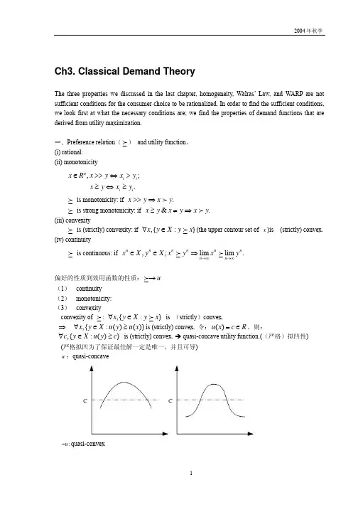
Ch3. Classical Demand TheoryThe three properties we discussed in the last chapter, homogeneity, Walras’ Law, and WARP are not sufficient conditions for the consumer choice to be rationalized. In order to find the sufficient conditions, we look first at what the necessary conditions are; we find the properties of demand functions that are derived from utility maximization.一、Preference relation ( ) and utility function 。
(i) rational: (ii) monotonicity,; .n i i i i x R x y x y x y x y ∈>>⇔>≥⇔≥is monotonicity: if .x y x y >>⇒is strong monotonicity: if &.x y x y x y ≥≠⇒(iii) convexityis (strictly) convexity: if ,{:}x y X y x ∀∈ (the upper contour set of x )is (strictly) convex. (iv) continuityis continuous: if ,;lim lim .nnnnnnn n x X y X x y x y →∞→∞∈∈⇒偏好的性质到效用函数的性质:u → (1) continuity (2) monotonicity:(3) convexity convexity of : ,{:}x y X y x ∀∈ is (strictly )convex.⇒ ,{:()()}x y X u y u x ∀∈≥is (strictly) convex. 令:()u x c R =∈,则:,{:()}c y X u y c ∀∈≥ is (strictly) convex. Î quasi-concave utility function.((严格)拟凹性)(严格拟凹为了保证最佳解一定是唯一,并且可导) u :quasi-concave:u −quasi-convexQuasi-concave and quasi-convex: monotone function; special e.g. line functionAnother proposition: if u is concave (convex) , f is strictly increasing, then f u is quasi-concave (quasi-convex).二、效用最大化问题(utility maximization problem )(UMP)1、 效用最大化问题 给定p ,w ,11max ()s.t. or (budget constraint)xn n u x px w px p x p x ≤=+⋅⋅⋅+性质1:只要u 是连续的,UMP 有解重写UMP {},max ()s.t. :,0xp w u x x B x px w x ∈=≤≥解的存在性和唯一性: B p,w 是闭集,并且有上下界,⇒B p,w 是紧集(compact set ),紧集上的连续函数最大化问题一定有解。
Questions for review1.Define the price elasticity of demand and the income elasticity of demand.需求价格弹性,是指一种物品需求量对其价格变动反应程度的衡量;需求收入弹性,是指一种物品需求量对消费者收入变动反应程度的衡量。
2.List and explain some of the determinants of the price elasticity of demand.需求的价格弹性取决于许多形成个人欲望的经济、社会和心理因素。
通常,需求价格弹性主要由以下几个因素决定:(1)必需品与奢侈品。
必需品倾向于需求缺乏弹性,奢侈品倾向于需求富有弹性。
(2)相似替代品的可获得性。
有相似替代品的物品往往富有需求弹性,因为消费者从这种物品转向其他物品较为容易。
(3)市场的定义。
范围小的市场的需求弹性往往大于范围大的市场,因为范围小的市场上的物品更容易找到相近的替代品。
(4)时间的长短。
物品往往随着时间变长而需求更富有弹性,因为在长期中人们有充分的时间来改变自己的消费嗜好和消费结构。
3.If the elasticity is greater than 1, is demand elastic or inelastic? If the elasticity equals 0, isdemand perfectly elastic or perfectly inelastic?弹性大于1,需求富有弹性。
弹性等于0,需求完全无弹性。
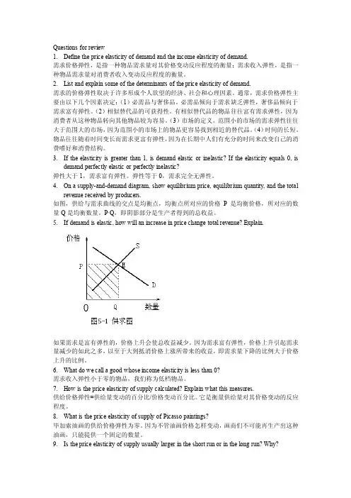
4.On a supply-and-demand diagram, show equilibrium price, equilibrium quantity, and the totalrevenue received by producers.如图,供给与需求曲线的交点是均衡点,均衡点所对应的价格P是均衡价格,所对应的数量Q是均衡数量。
第四章:供给与需求的市场力量&第五章:弹性及其应用名词解释:需求demand;买者愿意而且能购买的一种物品量供给supply:卖者愿意而且能够出售的一种物品量1需求定理law of demand:在其他条件相同时,(给定条件下,其他因素不变)一种物品价格上升,该物品需求量减少。
2供给定理:在其他条件相同时,一种物品价格上升,该物品供给量增加,当价格下降时,供给量减少。
3供求定理:任何一种物品价格的调整都会使该物品的供给与需求达到平衡。
4需求价格弹性price elasticity of demand:一种物品需求量对其价格变动反应程度的衡量,用需求量变动的百分比除以价格变动的百分比来计算。
5供给价格弹性:一种物品供给量对其价格变动反应程度的衡量,用供给量变动的百分比除以价格变动的百分比来计算。
6需求收入弹性:一种物品需求量对消费者收入变动反应程度的衡量,用需求量变动百分比除以收入变动百分比7交叉价格弹性:衡量一种物品需求量对另一种物品价格变动的反应程度,用第一种物品的需求量变动百分比除以第二种物品价格变动的百分比。
8均衡价格equilibrium price:使供给与需求平衡的价格。
9替代商品substitute:一种物品价格上升引起另一种物品需求量增加的两种物品10互补商品complement:一种物品价格上升引起另一种物品需求量减少的两种物品简答:1需求的影响因素?1收入2相关物品的价格3嗜好4预期5买者数量2供给的影响因素?1投入价格2技术3预期4卖者数量1.为什么需求曲线向右下方倾斜?2.需求价格弹性的决定因素:1.相近替代品的可获得性2.必需品与奢侈品3.市场的定义4.时间的长短3.供给价格弹性的决定因素:1.卖者改变他们生产的物品量的伸缩性2.所考虑的时间长短4.供求曲线变化如何影响价格并如何影响配置?5.均衡价格在市场配置中有何意义?发出价格信号6.当价格偏离均衡点时,如何自发的回到均衡价格?7.需求价格弹性的类型?(5种)&供给价格弹性的类型?计算题:1己知需求方程,求均衡价格?(二元一次方程)2在均衡点上,球需求价格弹性?(注意PQ的关系)第六章:供给、需求与政府政策名词解释:1价格上限price ceiling:可以出售一种物品的法定最高价格2价格下限price floor:可以出售一种物品的法定最低价格3税收负担的原理:a向买着征税:1税收影响需求,供给不受影响2需求曲线向左移动3比较新均衡, 说明税收的影响b向卖者征税:1直接影响供给2供给曲线向左移动3比较新均衡,说明税收影响关于税收的两个结论:1税收抑制了市场活动。
Syllabus for MicroeconomicsThe Nature of the Course:Specialized required courseSuitable Specialty: International economy and trade Marketing AccountingInformation Management and Systems Business AdministrationFinancial AdministrationCredit: 4Class Hours:64Authors:yijun liu ling langT he Purpose and Tasks of the CourseThis course is a basic professional course for undergraduate in the School of Business and Management. Through this course, students have a more comprehensive understanding of basic issues and basic viewpoints on the microeconomics. They can grasp the basic concepts of microeconomics, the basic idea, the basic analytical methods and basic theory as well. More important, lay ing a theoretical foundation for the further study of other professional courses.The Basic Requirements of the Course1.Require students to grasp the basic concept, the basic thought, the basic analysis method and the elementary theory of microeconomics.2.Require students to conduct self-study, and students are encouraged to widely read reference books to make it more understanding of basic economic theory and its application in all respects.3.Require teachers to pay close attention to using graphic tools and using mathematical tools properly.4.The advance curriculum is the higher mathematics.Outline the Content and Hours Allocation Recommendations Chapter 1Introduction 6 Class Hours §1 Ten Principles of Economics1.How People Make Decisions2. How People Interact3.How the Economy as a Whole Works§2 Thinking Like an Economist1.The Economist as a Scientist2. The Economist as a Policy Adviser3.Why Economist Disagree§3 the Using of Graphs in Economics (#)1.Graphic Drawing and Graphics Type in Economic Analysis2.Slope and Elasticity3. Note for Graphics Use in Economic Analysis§4 Interdependence and the Gains from Trade1.The Production Possibilities Frontier、Specialization and Tradeparative Advantage3.Applications of Comparative AdvantageChapter 2Supply and Demand(Ⅰ):How Markets Work 8 Class Hours §1Markets and Competitionpetitive Market2.Other Markets§2 law of demand1.Demand and the Demand Curve2.Shifts in the Demand Curve and Shift of the Demand Curve3.Market Demand and Individual Demand§3 law of supply (#)1. Supply and the Supply Curve2. Shifts in the Supply Curve and Shift of the Supply Curve3.Market Supply and Individual Supply§4 Supply and Demand Model1.The Conditions of Supply and Demand Model2.Supply and Demand Model3.What happens to equilibrium when supply and demand shifts?4.Cobweb Theory (☆)§5Elasticity and The Applications of Elasticity Theory1.the Elasticity of Demand and Its Application2.the Elasticity of Supply and Its Application(#)§6Supply、Demand and Government Policies1.Controls on prices (#)2.How Taxes Affect Market Outcomes3.Can Good News for Farming Be Bad News for Farmers?Exercise classes 2Class Hours Chapter 3 Supply and Demand(Ⅱ):Market and Welfare 16 Class Hours §1 The Theory of Consumer Choice 4 Class Hours1.Cardinal Utility Theory2. Preference Theory3.Application of The Theory of Consumer Choice§2 The Theory of Producer Choice 6 Class Hours1.The Organization of Production (#)2. Production Function and Factor Inputs3. The Cost Theory§3 Consumer Surplus 2Class Hours1.Willingness to Paying the Demand Curve to Measure Consumer Surplus3.How a Lower Price Raises Consumer Surplus§4 Producer Surplus(#)1.Cost and the Willingness to Sell2. Using the Supply Curve to Measure Producer Surplus3. How a Higher Price Raises Producer Surplus§5 Market Efficiency 2 Class Hours1.The Concept of Efficiency2.The Equilibrium Efficiency of the Competitive Firm(1)3.The conditions of the Efficient Competitive Firm§6 Application:The Cost of Taxation 2 Class Hours1.The Deadweight Loss of Taxation2.The Determinants of the Deadweight Loss3. Deadweight Loss and Tax Revenue as Taxes Vary§7 Application:International Trade (#)1.The Determinants of Trade2.The Winners and Losers from Trade3.The Arguments for Restricting TradeExercise classes 3 Class Hours Discussion class 1 Class Hour Chapter 4The Economics of the Public Sector 4 Class Hours §1 Externalities1.Externalities and Market Inefficiency2.Private Solutions to Externalities3.Public Policies toward Externalities§2 Public Goods and Common Resources1.The Different Kinds of Goods2.Public Goodsmon Resources§3 The Design of the Tax System(#)1.Taxes and Efficiency2.Taxes and EquityChapter 5 Supply and Demand(Ⅲ):Enterprise behavior and industrial organization8 Class Hours§1Types of Market (#)§2 Firms in Competitive Markets 4 Class Hours1. The Demand Curve and Revenue Curve of the Competitive Firm2. The Short-run Decision and the Supply Curve of the Competitive Firm3. The Short-run Supply Curve of the Competitive Market4.The Competitive Firm's Long-run Decision5.The Long-run Supply Curve of the Competitive Firm6.The Equilibrium Efficiency of the Competitive Firm(2)§3 Monopoly 4 Class Hours1.Why Monopolies Arise2.The Demand Curve and Revenue Curve of the Monopolistic Firm3.The Monopolistic Firm's Short-run and Long-run Decision4.The Welfare Cost of Monopoly5.Public Policy toward Monopolies6.Price Discrimination§4 Oligopoly (#)1.Markets with Only a few Sellers2.Game Theory and the Economics of Cooperation3.Public Policy toward Oligopolies§5 Monopolistic Competition(#)1.The Demand Curve and Revenue Curve of The MonopolisticCompetitive Firm2. The Monopolistic Competitive Firm in the Short-run and Long-run3. Monopolistic Competition and the Welfare of Society4.AdvertisingExercise classes 1 Class Hour Discussion class 1 Class Hour Chapter 6 Supply and Demand(Ⅳ):The Markets for the factors of production6 Class Hours§1 How Markets Determine Incomes1. Income and Wealth (#)2. Marginal Productivity Determines the Prices of Inputs§2 The Economics of Labor Market1.The Demand and Supply for Labor (#)2.Equilibrium in the Labor Market (#)3. Some Determinants of Equilibrium Wages4.The Economics of Discrimination§3 The Land Market and The Capital Marketnd and Rent2.Capital and Interest§4 Income Distribution (#)1.The Measurement of Inequality2.The Political Philosophy of Redistributing Income3.Policies to Reduce PovertyDiscussion class 2 Class Hours Chapter 7 Supply and Demand(Ⅴ):(General equilibrium) Market and Welfare (☆)§1 General equilibrium1.Meaning of the Equilibrium2. The Equilibrium Model of Léon Walras3. The Two-sector Model of General Equilibrium§2 Welfare Economics1.The Social Welfare Function2.Equity and EfficiencyChapter 8Uncertainty and Information (☆)§1 Uncertainty in the Economy1. Uncertainties and Risks2. The Effectiveness of Property3. Measurement of Risk Cost§2 Information, Risk and Markets1. Insurance and Risk-sharing2. Private Information and Market3. Risk Management in the Financial MarketsReview class 2 Class Hours Flexible time 4 Class Hours note:(#)Expressed that students learn these contents on its own, and they are included in the scope of examination.(☆)Expressed that students can choose according to their interest in reading, but not included in the scope of examination.Recommended Teaching Materials and Major Reference Books1.[美]曼昆著,梁小民译,《经济学原理(第5版)》,机械工业出版社,2009年2.[美]保罗·萨缪尔森、威廉·诺德豪斯著,萧琛主译,《经济学(第18版)》,人民邮电出版社,2008年3.刘毅军主编,《经济学基础》,石油工业出版社,2006年。
高级微观经济学1.需求经济学中需求是在一定的时期,在一既定的价格水平下,消费者愿意并且能够购买的商品数量。
需求显示了随着价钱升降而其它因素不变的情况下(ceteris paribus),某个体在每段时间内所愿意买的某货物的数量。
在某一价格下,消费者愿意购买的某一货物的总数量称为需求量。
在不同价格下,需求量会不同。
需求也就是说价格与需求量的关系。
2.供给经济学中的供给是指生产者在某一特定时期内,在每一价格水平上愿意并且能够提供的一定数量的商品或劳务。
3.均衡价格均衡价格是指一种商品需求量与供给量相等时的价格。
这时该商品的需求价格与供给价格相等称为均衡价格,该商品的需求量与供给量相等称为均衡数量。
4.效用效用是用来衡量消费者从一组商品和服务之中获得的幸福或者满足的尺度。
5.边际效用递减规律在一定时间内,在其他商品的消费数量保持不变的条件下,随着消费者对某种商品消费量的增加,消费者从该商品连续增加的每一消费单位中所得到的效用增量级边际替代效用是递减的。
6.预算约束线预算约束线又称预算线,消费可能线或等支出线,它表示在消费者收入和商品价格假定的条件下,消费者全部收入所能购买到的商品的不同数量组合。
7.收入消费曲线收入消费曲线是指在两种商品的价格水平之比为常数的情况下,每一收入水平所对应的两种商品最佳购买组合点组成的轨迹。
8.价格消费曲线价格消费曲线(Price Consumption Curve , PCC )是指在一种商品的价格水平和消费者收入水平为常数的情况下,另一种商品价格变动所对应的两种商品最佳购买组合点组成的轨迹。
也就是当某一种物品的价格改变时的消费组合。
9.吉芬商品所谓吉芬商品就是在其他因素不改变的情况下,当商品价格上升时,需求量增加,价格下降时,需求量减少。
10.生产函数生产函数是指在一定时期内,在技术水平不变的情况下,生产中所使用的各种生产要素的数量与所能生产的最大产量之间的关系。
生产函数反映的是在既定的生产技术条件下投入和产出之间的数量关系。
Chapter 5 Properties of DemandWhy? Theory – observable characteristics – testing – for future5.1 Relative prices and real incomez Money is a veil. Economists often prefer to measure important economicvariables in real, rather than nominal terms. z Relative pricesj ip p z Relative income jp wz Homogeneity and budget balancedness),1,...,,(),(0),(),(21nn n p w p p p p x w P x t tw tP x w P x =⇒>∀= ),(),(w P w w P Px ∀=5.2 The Slutsky equationz What do we expect from the theory of consumer? --- The law of demandClassical theory: the principle of diminishing marginal utilityz However, Giffen good! It is a product for which, among a poor population, a risein price will lead people to buy even more of the product. Possible examples: the potato in the Irish famine of 1845-1849[Figure 1.19]z Normal good and inferior goodThe “good” is the product for which demand increases in income.0),(>∂∂w w P x i The “bad” is … 0),(<∂∂w w P x iA Giffen good must be inferior, OR/AND an inferior good must be a Giffen good ??z Income effect and substitution effect IE SE TE +=Total effect : (price effect) measures the change of quantity demanded for a goodin response to a change in its price.Substitution effect : measures the effect of relative price change, in which theconsumer substitutes the relatively cheaper good for the relatively expensive good, and remains indifferent after the price change. Income effect :[Figure 1.20]z Theorem 5.1 The Slutsky equation :ww P x w P x p u P x p w P x ij j h i j i ∂∂−∂∂=∂∂∗),(),(),(),( Proof: from last chapter we know: *)),(,(*),(u P e P x u P x i h i =ji j i j h i p u P e w u P e P x p u P e P x p u P x ∂∂∂∂+∂∂=∂∂∗*),(*)),(,(*)),(,(),( w w P v P e u P e ==)),(,(*),(Shephard’s Lemma :)),(,(*),(*),(w P v P x u P x p u P e hj h j j==∂∂ ),()),(,(w P x w P v P x j h j =),(),(),(),(w P x w w P x p w P x p u P x j i j i j h i ∂∂+∂∂=∂∂⇒∗ww P x w P x p u P x p w P x ij j h i j i ∂∂−∂∂=∂∂⇒∗),(),(),(),(z Theorem 5.2 The law of demand :1. Hicksian demand: 0),(≤∂∂ih i p u P x (Negative Own-Substitution Terms)2. Marshallian demand: A decrease in the own price of a normal good will cause quantity demanded to increase. If an own price decrease causes a decrease in quantity demanded, the good must be inferior.Proof: using Shephard’s Lemma and the fact that the expenditure is a concave function. Hence…Classical theory vs. Modern theoryz Theorem 5.3 Symmetric, negative semidefinite (Hicksian) substitutionmatrix()⎟⎟⎟⎟⎟⎟⎠⎞⎜⎜⎜⎜⎜⎜⎝⎛∂∂∂∂∂∂∂∂≡n h n h n n h h p u P x p u P x p u P x p u P x u P ),(...),(:::),(...),(,1111σProof: 1) The order of differentiation of the expenditure function makes nodifference! i j j i p p u P e p p u P e ∂∂∂=∂∂∂),(),(22ihj j h i p u P x p u P x ∂∂=∂∂⇒),(),( 2) ()u P ,σ is simply the Hessian matrix of second-order price partials ofthe expenditure function.z Slutsky matrix⎟⎟⎟⎟⎟⎠⎞⎜⎜⎜⎜⎜⎝⎛∂∂+∂∂∂∂+∂∂∂∂+∂∂∂∂+∂∂),(),(),(...),(),(),(:::),(),(),(...),(),(),(11111111w P x w w P x p w P x w P x w w P x p w P x w P x w w P x p w P x w P x w w P x p w P x n n n n n n n n5.3 Some Elasticity Relationsz A general formula for elasticity: yxx y y x y x e xy ln ln %%∂∂=∂∂=∆∆=z Income Elasticity ),(),(w P x ww w P x i i i ∂∂≡ηz Price Elasticity ),(),(w P x p p w P x i jj i ij ∂∂≡εz Aggregation in consumer demand, where income share10),(=≥≡∑i ii i i i sands ww P x p sEngel aggregation: ∑==ni i i s 11η Cournot aggregation: ∑=−=ni j iji s s 1ε5.4 Integrabilityz We ask a question: if we observe a demand function ),(w P x that has theseproperties (homogeneous of degree zero, satisfy Walras’ law, and have a symmetric and negative semidefinite Slutsky matrix), can we find preferences that rationalize ),(w P x ?-- This integrability problem has a long tradition, beginning with Antonelli 1886.z Why we ask such question?1. On a theoretical level, the properties of demand (homogeneity of degree one,satisfaction of Walras’ law, and a symmetric and negative semidefinite substitution matrix) are not only necessary consequences of the preference-based demand theory, but these are also all of the consequences. As long as consumer demand satisfies these properties, there is some rational preference relation that could have generated this demand.2. The result completes our study of the relation between the preference-basedtheory of demand and the choice-based theory of demand. In general, demand satisfying the weak axiom cannot be rationalized by preferences, because the substitution matrix could be not symmetric. Hence, the result here shows us, that the only thing added to the properties of demand by the rational preference hypothesis, beyond what is implied by the weak axiom, homogeneity of degree one, and Walras’ law, is symmetry of the substitution matrix.3. On a practical level, the result tells us how and when we can recover theinformation of preferences from observation of the consumer’s demand behavior. 4. In empirical studies, it allows us to begin by specifying a tractable demandfunction and then check whether it satisfies the necessary and sufficient conditions. We need not derive the utility function. zTwo steps to recover preferences from demand:1. recovering preferences from the expenditure function ),(u P eTheorem 5.4 Constructing a utility function from an expenditure functionLet ),(w P e be a function satisfying all properties of an expenditure function, then we can construct a utility function by {})(|0max )(u A x u x u ∈≥≡, where{}0),(|)(>>∀≥∈≡+P u P e Px R x u A n2. recovering an expenditure function from ),(w P xTheorem 5.5 Constructing an expenditure function from a demand functionThe necessary and sufficient condition for the recovery of an underlying expenditure function is the symmetric and negative semidefiniteness of the Slutsky equation.At first, we consider the case of two goods. Suppose 12=p without loss of generality, pick an arbitrary point ),,1,(0001u w p .We will now recover the value of the expenditure function 0),1,(101>∀p u p e from following differential equation (to integrate):))(,(),()(1111111p e p x u p x dp p de h == with the initial condition 001)(w p e = For the general case of L commodities, we have a system of partial differential equations:))(,()(...))(,()(11P e P x p P e P e P x p P e L L=∂∂=∂∂ The existence of a solution to above system is guaranteed when 2>L if and only ifits Hessian matrix )(2P e D p is symmetric. ( Frobenius’ theorem)In addition, if a solution exists, as long as ),(w P S is negative semidefinite, it will possess the properties of an expenditure function.The intuition: by changing prices one at a time, we can decompose this problem into L subproblems where only one price changes at each step. Hence, the symmetry of Slutsky matrix implies that the value of expenditure function should not depend on the particular path from the original price to the new price.Example:Suppose there are three goods, the demand function is as follows:3,2,1,),,,(321==i p ww p p p x ii i α, where 1,0321=++>ααααand iWe want to find ()u p p p e ,,,321.We have:()()()321321332211213333122232111321321321)(),()()ln()ln()ln()),(ln(),,()ln()),(ln(),,()ln()),(ln(),,()ln()),(ln(3,2,1,,,,ln 3,2,1,,,,,,,αααααααααααp p p u c u P e u c p p p u P e u p p c p u P e u p p c p u P e u p p c p u P e i p p u p p p e i p u p p p e p u p p p e i i ii i i =⇒+++=⇒⎪⎩⎪⎨⎧+=+=+=⇒==∂∂⇒==∂∂Because the implied demand behavior is independent of strictly increasing transformation, we can choose u u c =)(.Recover a utility function from this expenditure function.{})(|0max )(u A x u x u ∈≥≡, where {}0),(|)(>>∀≥∈≡+P u P e Px R x u A n321321321321),(ααααααp p p Pxu p p up u P e Px ≤⇔=≥ Hence ()321321332211αααp p p x p x p x p x u ++=5.5Welfare analysis。