Divide and Conquer in Granular Computing Topological Partitions

@ @ Exercises
Computing Wishes and Proposals † Computer Algebra Systems
@ @ Solutions
100 Proposals for Problems to Tackle † Sources of Interesting and Challenging Problems † ISSAC Challenge Problems † 100$–100-Digit Challenge
@ @ References
CHAPTER
2
Structure of Mathematica Expressions
2.0 Remarks 2.1 Expressions
Everything Is an Expression † Hierarchical Structure of Symbolic Expressions † Formatting Possibilities † Traditional Mathematics Notation versus Computer Mathematics Notation † Typeset Forms † Heads and Arguments † Symbols † Nested Heads † Input Form and the Formatting of Programs
Contents
PREFACE
to The Mathematica GuideBooks
CHAPTER 0

Introduction and Orientation
0.1 Overview 0.1.1 Content Summaries 0.1.2 Relation of the Four Volumes 0.1.3 Chapter Structure 0.1.4 Code Presentation Style 0.2 Requirements 0.2.1 Hardware and Software 0.2.2 Reader Prerequisites 0.3 What the GuideBooks Are and What They Are Not 0.3.1 Doing Computer Mathematics 0.3.2 Programming Paradigms 0.4 Exercises and Solutions 0.4.1 Exercises 0.4.2 Solutions 0.5 The Books Versus the Electronic Components 0.5.1 Working with the Notebook 0.5.2 Reproducibility of the Results 0.5.3 Earlier Versions of the Notebooks 0.6 Style and Design Elements 0.6.1 Text and Code Formatting 0.6.2 References 0.6.3 Variable Scoping, Input Numbering, and Warning Messages 0.6.4 Graphics 0.6.5 Notations and Symbols 0.6.6 Units 0.6.7 Cover Graphics

一个域到实数域内的一种映射。它是通常绝对值的推广。若φ是由域F到实数域R的映射，称φ为F上的一个 绝对值，若φ满足条件：
1、φ(a)≥0，φ(a)=0，当且仅当a=0（F的零元）； 2、φ(ab)=φ(a)φ(b)； 3、φ(a+b)≤Cmax{φ(a),φ(b)}，其中a，b∈F，C为一常数，满足0<C≤2； 注意由条件1,2,3可推出三角不等式，即 4、φ(a+b)≤φ(a)+φ(b)； 并且条件1,2,3与条件1,2,4是等价的。最常见的绝对值有：通常实数域的绝对值|·|，复数域上的模。
概念基础
赋值论
绝对值
域论的一个重要分支，它是研究交换代数的一个工具，特别是在代数数论、分歧理论、类域论和代数几何中 有极为重要的应用。通常的赋值可分为加法与乘法赋值两类，有时简称赋值。从赋值出发，可以给原来的域一个 拓扑结构，使之成为拓扑域。赋值理论肇始于屈尔沙克于1913年发表的论文。赋值、赋值域这些名词都是他首先 引入的。气候，经过奥斯特洛夫斯基（Ostrowski，A.M.）等人的工作，解决了屈尔沙克在论文中提出的问题， 并发展了这一理论。1932年，克鲁尔（Krull，W.）发表了题为《一般赋值理论》的基本论文，从而奠定了赋值 论这一分支的基础。时至今日，赋值理论已逐渐越出了“域”的界限，在许多代数结构上，例如群、环、向量空 间等，也用多种方式引进赋值，并由此对这些结构作算术理论的研究。此外，赋值论还渗入泛函分析的领域，发 展了所谓非阿基米德泛函分析。
谢谢观看
非阿基米德绝对值
数学术语
目录
01 概念基础
02
03 阿基米德绝对值
非阿基米德绝对值(non-Archimedean absolute value)亦称一阶赋值，是一类特殊的绝对值。与其相排斥 的为阿基米德绝对值。把绝对值区分为阿基米德绝对值和非阿基米德绝对值，来自奥斯特洛夫斯基(Ostrowski, A. M.)于1915chimedean absolute value)是与非阿基米德绝对值相排斥的另一种绝对值。设φ为F上 的绝对值，若φ满足三角不等式

1毛利Gross profit/margin商业企业商品销售收入减去商品原进价后的余额。

净利的对称，又称商品进销差价。

因其尚未减去商品流通费和税金，还不是净利，故称毛利。

毛利率的计算是：（不含税销售收入-不含税成本）/不含税销售收入。

假定某商品成本单价为12元（不含税），售价为15元（不含税），则该商品毛利率=（15-12）/15=20%商品流通企业计算公式：毛利=不含税售价-不含税进价生产制造企业计算公式：毛利=产品销售收入-生产成本(即财务报表中的营业成本）2 普通分数（common fraction）的定义是什么？分子分母均为整数的分数，如123/7963。

同时，分母不可为1或0 common fraction可以是简分数，但简分数不一定是普通分数。

简分数的定义是分子和分母的公因数是1，比如4/194/6是一个普通分数，但不是简分数4/7是一个普通分数，也是简分数3 红利：dividend上市公司在进行利润分配时，分配给股东的利润。

一般是每10股，派发XX元，股东在获得时，还要扣调上交税额。

普通股股东所得到的超过股息部分的利润，称为红利。

普通股股东所得红利没有固定数额，企业分派给股东多少红利，则取决于企业年度经营状的好坏和企业今后经营发展战略决策的总体安排。

4 四分位数Quartile四分位数（Quartile），即统计学中，把所有数值由小到大排列并分成四等份，处于三个分割点位置的得分就是四分位数。

第一四分位数(Q1)，又称“较小四分位数”，等于该样本中所有数值由小到大排列后第25%的数字。

小到大排列后第50%的数字。

第三四分位数(Q3)，又称“较大四分位数”，等于该样本中所有数值由小到大排列后第75%的数字。

第三四分位数与第一四分位数的差距又称四分位距（InterQuartile Range, IQR）。

首先确定四分位数的位置：Q1的位置=（n+1）/4Q2的位置=（n+1）/2Q3的位置=3（n+1）/4n表示项数实例1数据总量: 6, 47, 49, 15, 42, 41, 7, 39, 43, 40, 36由小到大排列的结果: 6, 7, 15, 36, 39, 40, 41, 42, 43, 47, 49一共11项Q1 的位置=（11+1）/4=3 Q2 的位置=（11+1）/2=6 Q3的位置=3（11+1）/4=9Q1 = 15，Q2 = 40，Q3 = 43实例2数据总量: 7, 15, 36, 39, 40, 41一共6项Q1 的位置=（6+1）/4=1.75 Q2 的位置=（6+1）/2=3.5 Q3的位置=3（6+1）/4=5.25Q1 = 7+（15-7）×（1.75-1）=13，Q2 = 36+（39-36）×（3.5-3）=37.5，Q3 = 40+（41-40）×（5.25-5）=40.25将n个数从小到大排列：Q2为n个数组成的数列的中数（Median）；当n为奇数时，中数Q2将该数列分为数量相等的两组数，每组有(n-1)/2 个数，Q1为第一组(n-1)/2 个数的中数，Q3为为第二组(n-1)/2个数的中数；当n为偶数时，中数Q2将该数列分为数量相等的两组数，每组有n/2个数，Q1为第一组n/2 个数的中数，Q3为为第二组n/2 个数的中数。

著名数学家的翻译名
数学是我们学好其他自然学科（如物理、化学、生物、天文学等）的基础，更是在日常生活中起着不可替代的作用。

在数学的学习教材中，经常会见到一些英文字母的外国数学家名字。

偶在闲暇时，为数学爱好着，整理了一下他们的翻译名字，以便大家更好地学习。

Weierstrass 魏尔斯特拉斯
Cantor 康托尔
Bernoulli 伯努力
Fatou 法都
Green 格林
S.Lie 李
Euler 欧拉
Gauss 高斯
Riemann 黎曼
Caratheodory 卡拉西奥多礼
Newton 牛顿
Jordan 约当
Laplace 拉普拉斯
Riesz 黎茨
Fourier 傅立叶
Borel 波莱尔
Dirchlet 狄利克雷
Lebesgue 勒贝格
Leibniz 莱不尼兹
Abel 阿贝尔
Lagrange 拉格朗日
Ljapunov 李雅普诺夫
Holder 赫尔得
Poisson 泊松
H.Hopf 霍普夫
Baire 贝尔
Fermat 费马
Taylor 泰勒
Schauder 肖德尔
Lipschiz 李普西茨
Liouville 刘维尔
Lindelof 林德洛夫
de Moivre 棣莫佛
Klein 克莱因
Bessel 贝塞尔
Euclid 欧几里德
Chebyschev 切比雪夫Banach 巴拿赫Hilbert 希尔伯特Minkowski 闵可夫斯基Hamilton 哈密尔顿Poincare 彭加莱。

离散数学中英⽂名词对照表离散数学中英⽂名词对照表外⽂中⽂AAbel category Abel 范畴Abel group (commutative group) Abel 群(交换群)Abel semigroup Abel 半群accessibility relation 可达关系action 作⽤addition principle 加法原理adequate set of connectives 联结词的功能完备（全）集adjacent 相邻（邻接）adjacent matrix 邻接矩阵adjugate 伴随adjunction 接合affine plane 仿射平⾯algebraic closed field 代数闭域algebraic element 代数元素algebraic extension 代数扩域（代数扩张）almost equivalent ⼏乎相等的alternating group 三次交代群annihilator 零化⼦antecedent 前件anti symmetry 反对称性anti-isomorphism 反同构arboricity 荫度arc set 弧集arity 元数arrangement problem 布置问题associate 相伴元associative algebra 结合代数associator 结合⼦asymmetric 不对称的(⾮对称的)atom 原⼦atomic formula 原⼦公式augmenting digeon hole principle 加强的鸽⼦笼原理augmenting path 可增路automorphism ⾃同构automorphism group of graph 图的⾃同构群auxiliary symbol 辅助符号axiom of choice 选择公理axiom of equality 相等公理axiom of extensionality 外延公式axiom of infinity ⽆穷公理axiom of pairs 配对公理axiom of regularity 正则公理axiom of replacement for the formula Ф关于公式Ф的替换公式axiom of the empty set 空集存在公理axiom of union 并集公理Bbalanced imcomplete block design 平衡不完全区组设计barber paradox 理发师悖论base 基Bell number Bell 数Bernoulli number Bernoulli 数Berry paradox Berry 悖论bijective 双射bi-mdule 双模binary relation ⼆元关系binary symmetric channel ⼆进制对称信道binomial coefficient ⼆项式系数binomial theorem ⼆项式定理binomial transform ⼆项式变换bipartite graph ⼆分图block 块block 块图（区组）block code 分组码block design 区组设计Bondy theorem Bondy 定理Boole algebra Boole 代数Boole function Boole 函数Boole homomorophism Boole 同态Boole lattice Boole 格bound occurrence 约束出现bound variable 约束变量bounded lattice 有界格bridge 桥Bruijn theorem Bruijn 定理Burali-Forti paradox Burali-Forti 悖论Burnside lemma Burnside 引理Ccage 笼canonical epimorphism 标准满态射Cantor conjecture Cantor 猜想Cantor diagonal method Cantor 对⾓线法Cantor paradox Cantor 悖论cardinal number 基数Cartesion product of graph 图的笛卡⼉积Catalan number Catalan 数category 范畴Cayley graph Cayley 图Cayley theorem Cayley 定理center 中⼼characteristic function 特征函数characteristic of ring 环的特征characteristic polynomial 特征多项式check digits 校验位Chinese postman problem 中国邮递员问题chromatic number ⾊数chromatic polynomial ⾊多项式circuit 回路circulant graph 循环图circumference 周长class 类classical completeness 古典完全的classical consistent 古典相容的clique 团clique number 团数closed term 闭项closure 闭包closure of graph 图的闭包code 码code element 码元code length 码长code rate 码率code word 码字coefficient 系数coimage 上象co-kernal 上核coloring 着⾊coloring problem 着⾊问题combination number 组合数combination with repetation 可重组合common factor 公因⼦commutative diagram 交换图commutative ring 交换环commutative seimgroup 交换半群complement 补图(⼦图的余) complement element 补元complemented lattice 有补格complete bipartite graph 完全⼆分图complete graph 完全图complete k-partite graph 完全k-分图complete lattice 完全格composite 复合composite operation 复合运算composition (molecular proposition) 复合（分⼦）命题composition of graph (lexicographic product)图的合成（字典积）concatenation (juxtaposition) 邻接运算concatenation graph 连通图congruence relation 同余关系conjunctive normal form 正则合取范式connected component 连通分⽀connective 连接的connectivity 连通度consequence 推论（后承）consistent (non-contradiction) 相容性（⽆⽭盾性）continuum 连续统contraction of graph 图的收缩contradiction ⽭盾式（永假式）contravariant functor 反变函⼦coproduct 上积corank 余秩correct error 纠正错误corresponding universal map 对应的通⽤映射countably infinite set 可列⽆限集（可列集）covariant functor (共变)函⼦covering 覆盖covering number 覆盖数Coxeter graph Coxeter 图crossing number of graph 图的叉数cuset 陪集cotree 余树cut edge 割边cut vertex 割点cycle 圈cycle basis 圈基cycle matrix 圈矩阵cycle rank 圈秩cycle space 圈空间cycle vector 圈向量cyclic group 循环群cyclic index 循环（轮转）指标cyclic monoid 循环单元半群cyclic permutation 圆圈排列cyclic semigroup 循环半群DDe Morgan law De Morgan 律decision procedure 判决过程decoding table 译码表deduction theorem 演绎定理degree 次数,次(度)degree sequence 次(度)序列derivation algebra 微分代数Descartes product Descartes 积designated truth value 特指真值detect errer 检验错误deterministic 确定的diagonal functor 对⾓线函⼦diameter 直径digraph 有向图dilemma ⼆难推理direct consequence 直接推论（直接后承）direct limit 正向极限direct sum 直和directed by inclution 被包含关系定向discrete Fourier transform 离散 Fourier 变换disjunctive normal form 正则析取范式disjunctive syllogism 选⾔三段论distance 距离distance transitive graph 距离传递图distinguished element 特异元distributive lattice 分配格divisibility 整除division subring ⼦除环divison ring 除环divisor (factor) 因⼦domain 定义域Driac condition Dirac 条件dual category 对偶范畴dual form 对偶式dual graph 对偶图dual principle 对偶原则(对偶原理) dual statement 对偶命题dummy variable 哑变量（哑变元）Eeccentricity 离⼼率edge chromatic number 边⾊数edge coloring 边着⾊edge connectivity 边连通度edge covering 边覆盖edge covering number 边覆盖数edge cut 边割集edge set 边集edge-independence number 边独⽴数eigenvalue of graph 图的特征值elementary divisor ideal 初等因⼦理想elementary product 初等积elementary sum 初等和empty graph 空图empty relation 空关系empty set 空集endomorphism ⾃同态endpoint 端点enumeration function 计数函数epimorphism 满态射equipotent 等势equivalent category 等价范畴equivalent class 等价类equivalent matrix 等价矩阵equivalent object 等价对象equivalent relation 等价关系error function 错误函数error pattern 错误模式Euclid algorithm 欧⼏⾥德算法Euclid domain 欧⽒整环Euler characteristic Euler 特征Euler function Euler 函数Euler graph Euler 图Euler number Euler 数Euler polyhedron formula Euler 多⾯体公式Euler tour Euler 闭迹Euler trail Euler 迹existential generalization 存在推⼴规则existential quantifier 存在量词existential specification 存在特指规则extended Fibonacci number ⼴义 Fibonacci 数extended Lucas number ⼴义Lucas 数extension 扩充（扩张）extension field 扩域extension graph 扩图exterior algebra 外代数Fface ⾯factor 因⼦factorable 可因⼦化的factorization 因⼦分解faithful (full) functor 忠实（完满）函⼦Ferrers graph Ferrers 图Fibonacci number Fibonacci 数field 域filter 滤⼦finite extension 有限扩域finite field (Galois field ) 有限域（Galois 域）finite dimensional associative division algebra有限维结合可除代数finite set 有限（穷）集finitely generated module 有限⽣成模first order theory with equality 带符号的⼀阶系统five-color theorem 五⾊定理five-time-repetition 五倍重复码fixed point 不动点forest 森林forgetful functor 忘却函⼦four-color theorem(conjecture) 四⾊定理（猜想）F-reduced product F-归纳积free element ⾃由元free monoid ⾃由单元半群free occurrence ⾃由出现free R-module ⾃由R-模free variable ⾃由变元free-?-algebra ⾃由?代数function scheme 映射格式GGalileo paradox Galileo 悖论Gauss coefficient Gauss 系数GBN (G?del-Bernays-von Neumann system)GBN系统generalized petersen graph ⼴义 petersen 图generating function ⽣成函数generating procedure ⽣成过程generator ⽣成⼦（⽣成元）generator matrix ⽣成矩阵genus 亏格girth （腰）围长G?del completeness theorem G?del 完全性定理golden section number 黄⾦分割数（黄⾦分割率）graceful graph 优美图graceful tree conjecture 优美树猜想graph 图graph of first class for edge coloring 第⼀类边⾊图graph of second class for edge coloring 第⼆类边⾊图graph rank 图秩graph sequence 图序列greatest common factor 最⼤公因⼦greatest element 最⼤元（素）Grelling paradox Grelling 悖论Gr?tzsch graph Gr?tzsch 图group 群group code 群码group of graph 图的群HHajós conjecture Hajós 猜想Hamilton cycle Hamilton 圈Hamilton graph Hamilton 图Hamilton path Hamilton 路Harary graph Harary 图Hasse graph Hasse 图Heawood graph Heawood 图Herschel graph Herschel 图hom functor hom 函⼦homemorphism 图的同胚homomorphism 同态（同态映射）homomorphism of graph 图的同态hyperoctahedron 超⼋⾯体图hypothelical syllogism 假⾔三段论hypothese (premise) 假设(前提)Iideal 理想identity 单位元identity natural transformation 恒等⾃然变换imbedding 嵌⼊immediate predcessor 直接先⾏immediate successor 直接后继incident 关联incident axiom 关联公理incident matrix 关联矩阵inclusion and exclusion principle 包含与排斥原理inclusion relation 包含关系indegree ⼊次（⼊度）independent 独⽴的independent number 独⽴数independent set 独⽴集independent transcendental element 独⽴超越元素index 指数individual variable 个体变元induced subgraph 导出⼦图infinite extension ⽆限扩域infinite group ⽆限群infinite set ⽆限（穷）集initial endpoint 始端initial object 初始对象injection 单射injection functor 单射函⼦injective (one to one mapping) 单射（内射）inner face 内⾯inner neighbour set 内（⼊）邻集integral domain 整环integral subdomain ⼦整环internal direct sum 内直和intersection 交集intersection of graph 图的交intersection operation 交运算interval 区间invariant factor 不变因⼦invariant factor ideal 不变因⼦理想inverse limit 逆向极限inverse morphism 逆态射inverse natural transformation 逆⾃然变换inverse operation 逆运算inverse relation 逆关系inversion 反演isomorphic category 同构范畴isomorphism 同构态射isomorphism of graph 图的同构join of graph 图的联JJordan algebra Jordan 代数Jordan product (anti-commutator) Jordan乘积（反交换⼦）Jordan sieve formula Jordan 筛法公式j-skew j-斜元juxtaposition 邻接乘法Kk-chromatic graph k-⾊图k-connected graph k-连通图k-critical graph k-⾊临界图k-edge chromatic graph k-边⾊图k-edge-connected graph k-边连通图k-edge-critical graph k-边临界图kernel 核Kirkman schoolgirl problem Kirkman ⼥⽣问题Kuratowski theorem Kuratowski 定理Llabeled graph 有标号图Lah number Lah 数Latin rectangle Latin 矩形Latin square Latin ⽅lattice 格lattice homomorphism 格同态law 规律leader cuset 陪集头least element 最⼩元least upper bound 上确界（最⼩上界）left (right) identity 左（右）单位元left (right) invertible element 左（右）可逆元left (right) module 左（右）模left (right) zero 左（右）零元left (right) zero divisor 左（右）零因⼦left adjoint functor 左伴随函⼦left cancellable 左可消的left coset 左陪集length 长度Lie algebra Lie 代数line- group 图的线群logically equivanlent 逻辑等价logically implies 逻辑蕴涵logically valid 逻辑有效的（普效的）loop 环Lucas number Lucas 数Mmagic 幻⽅many valued proposition logic 多值命题逻辑matching 匹配mathematical structure 数学结构matrix representation 矩阵表⽰maximal element 极⼤元maximal ideal 极⼤理想maximal outerplanar graph 极⼤外平⾯图maximal planar graph 极⼤平⾯图maximum matching 最⼤匹配maxterm 极⼤项（基本析取式）maxterm normal form(conjunctive normal form) 极⼤项范式（合取范式）McGee graph McGee 图meet 交Menger theorem Menger 定理Meredith graph Meredith 图message word 信息字mini term 极⼩项minimal κ-connected graph 极⼩κ-连通图minimal polynomial 极⼩多项式Minimanoff paradox Minimanoff 悖论minimum distance 最⼩距离Minkowski sum Minkowski 和minterm (fundamental conjunctive form) 极⼩项（基本合取式）minterm normal form(disjunctive normal form)极⼩项范式（析取范式）M?bius function M?bius 函数M?bius ladder M?bius 梯M?bius transform (inversion) M?bius 变换（反演）modal logic 模态逻辑model 模型module homomorphism 模同态(R-同态)modus ponens 分离规则modus tollens 否定后件式module isomorphism 模同构monic morphism 单同态monoid 单元半群monomorphism 单态射morphism (arrow) 态射（箭）M?bius function M?bius 函数M?bius ladder M?bius 梯M?bius transform (inversion) M?bius 变换（反演）multigraph 多重图multinomial coefficient 多项式系数multinomial expansion theorem 多项式展开定理multiple-error-correcting code 纠多错码multiplication principle 乘法原理mutually orthogonal Latin square 相互正交拉丁⽅Nn-ary operation n-元运算n-ary product n-元积natural deduction system ⾃然推理系统natural isomorphism ⾃然同构natural transformation ⾃然变换neighbour set 邻集next state 下⼀个状态next state transition function 状态转移函数non-associative algebra ⾮结合代数non-standard logic ⾮标准逻辑Norlund formula Norlund 公式normal form 正规形normal model 标准模型normal subgroup (invariant subgroup) 正规⼦群（不变⼦群）n-relation n-元关系null object 零对象nullary operation 零元运算Oobject 对象orbit 轨道order 阶order ideal 阶理想Ore condition Ore 条件orientation 定向orthogonal Latin square 正交拉丁⽅orthogonal layout 正交表outarc 出弧outdegree 出次(出度)outer face 外⾯outer neighbour 外（出）邻集outerneighbour set 出(外)邻集outerplanar graph 外平⾯图Ppancycle graph 泛圈图parallelism 平⾏parallelism class 平⾏类parity-check code 奇偶校验码parity-check equation 奇偶校验⽅程parity-check machine 奇偶校验器parity-check matrix 奇偶校验矩阵partial function 偏函数partial ordering (partial relation) 偏序关系partial order relation 偏序关系partial order set (poset) 偏序集partition 划分,分划,分拆partition number of integer 整数的分拆数partition number of set 集合的划分数Pascal formula Pascal 公式path 路perfect code 完全码perfect t-error-correcting code 完全纠-错码perfect graph 完美图permutation 排列（置换）permutation group 置换群permutation with repetation 可重排列Petersen graph Petersen 图p-graph p-图Pierce arrow Pierce 箭pigeonhole principle 鸽⼦笼原理planar graph （可）平⾯图plane graph 平⾯图Pólya theorem Pólya 定理polynomail 多项式polynomial code 多项式码polynomial representation 多项式表⽰法polynomial ring 多项式环possible world 可能世界power functor 幂函⼦power of graph 图的幂power set 幂集predicate 谓词prenex normal form 前束范式pre-ordered set 拟序集primary cycle module 准素循环模prime field 素域prime to each other 互素primitive connective 初始联结词primitive element 本原元primitive polynomial 本原多项式principal ideal 主理想principal ideal domain 主理想整环principal of duality 对偶原理principal of redundancy 冗余性原则product 积product category 积范畴product-sum form 积和式proof (deduction) 证明（演绎）proper coloring 正常着⾊proper factor 真正因⼦proper filter 真滤⼦proper subgroup 真⼦群properly inclusive relation 真包含关系proposition 命题propositional constant 命题常量propositional formula(well-formed formula,wff)命题形式（合式公式）propositional function 命题函数propositional variable 命题变量pullback 拉回(回拖) pushout 推出Qquantification theory 量词理论quantifier 量词quasi order relation 拟序关系quaternion 四元数quotient (difference) algebra 商（差）代数quotient algebra 商代数quotient field (field of fraction) 商域（分式域）quotient group 商群quotient module 商模quotient ring (difference ring , residue ring) 商环（差环，同余类环）quotient set 商集RRamsey graph Ramsey 图Ramsey number Ramsey 数Ramsey theorem Ramsey 定理range 值域rank 秩reconstruction conjecture 重构猜想redundant digits 冗余位reflexive ⾃反的regular graph 正则图regular representation 正则表⽰relation matrix 关系矩阵replacement theorem 替换定理representation 表⽰representation functor 可表⽰函⼦restricted proposition form 受限命题形式restriction 限制retraction 收缩Richard paradox Richard 悖论right adjoint functor 右伴随函⼦right cancellable 右可消的right factor 右因⼦right zero divison 右零因⼦ring 环ring of endomorphism ⾃同态环ring with unity element 有单元的环R-linear independence R-线性⽆关root field 根域rule of inference 推理规则Russell paradox Russell 悖论Ssatisfiable 可满⾜的saturated 饱和的scope 辖域section 截⼝self-complement graph ⾃补图semantical completeness 语义完全的（弱完全的）semantical consistent 语义相容semigroup 半群separable element 可分元separable extension 可分扩域sequent ⽮列式sequential 序列的Sheffer stroke Sheffer 竖（谢弗竖）simple algebraic extension 单代数扩域simple extension 单扩域simple graph 简单图simple proposition (atomic proposition) 简单（原⼦）命题simple transcental extension 单超越扩域simplication 简化规则slope 斜率small category ⼩范畴smallest element 最⼩元（素）Socrates argument Socrates 论断（苏格拉底论断）soundness (validity) theorem 可靠性（有效性）定理spanning subgraph ⽣成⼦图spanning tree ⽣成树spectra of graph 图的谱spetral radius 谱半径splitting field 分裂域standard model 标准模型standard monomil 标准单项式Steiner triple Steiner 三元系⼤集Stirling number Stirling 数Stirling transform Stirling 变换subalgebra ⼦代数subcategory ⼦范畴subdirect product ⼦直积subdivison of graph 图的细分subfield ⼦域subformula ⼦公式subdivision of graph 图的细分subgraph ⼦图subgroup ⼦群sub-module ⼦模subrelation ⼦关系subring ⼦环sub-semigroup ⼦半群subset ⼦集substitution theorem 代⼊定理substraction 差集substraction operation 差运算succedent 后件surjection (surjective) 满射switching-network 开关⽹络Sylvester formula Sylvester公式symmetric 对称的symmetric difference 对称差symmetric graph 对称图symmetric group 对称群syndrome 校验⼦syntactical completeness 语法完全的（强完全的）Syntactical consistent 语法相容system ?3 , ?n , ??0 , ??系统?3 , ?n , ??0 , ??system L 公理系统 Lsystem ?公理系统?system L1 公理系统 L1system L2 公理系统 L2system L3 公理系统 L3system L4 公理系统 L4system L5 公理系统 L5system L6 公理系统 L6system ?n 公理系统?nsystem of modal prepositional logic 模态命题逻辑系统system Pm 系统 Pmsystem S1 公理系统 S1system T (system M) 公理系统 T(系统M)Ttautology 重⾔式（永真公式）technique of truth table 真值表技术term 项terminal endpoint 终端terminal object 终结对象t-error-correcing BCH code 纠 t -错BCH码theorem (provable formal) 定理（可证公式）thickess 厚度timed sequence 时间序列torsion 扭元torsion module 扭模total chromatic number 全⾊数total chromatic number conjecture 全⾊数猜想total coloring 全着⾊total graph 全图total matrix ring 全⽅阵环total order set 全序集total permutation 全排列total relation 全关系tournament 竞赛图trace (trail) 迹tranformation group 变换群transcendental element 超越元素transitive 传递的tranverse design 横截设计traveling saleman problem 旅⾏商问题tree 树triple system 三元系triple-repetition code 三倍重复码trivial graph 平凡图trivial subgroup 平凡⼦群true in an interpretation 解释真truth table 真值表truth value function 真值函数Turán graph Turán 图Turán theorem Turán 定理Tutte graph Tutte 图Tutte theorem Tutte 定理Tutte-coxeter graph Tutte-coxeter 图UUlam conjecture Ulam 猜想ultrafilter 超滤⼦ultrapower 超幂ultraproduct 超积unary operation ⼀元运算unary relation ⼀元关系underlying graph 基础图undesignated truth value ⾮特指值undirected graph ⽆向图union 并(并集)union of graph 图的并union operation 并运算unique factorization 唯⼀分解unique factorization domain (Gauss domain) 唯⼀分解整域unique k-colorable graph 唯⼀k着⾊unit ideal 单位理想unity element 单元universal 全集universal algebra 泛代数（Ω代数）universal closure 全称闭包universal construction 通⽤结构universal enveloping algebra 通⽤包络代数universal generalization 全称推⼴规则universal quantifier 全称量词universal specification 全称特指规则universal upper bound 泛上界unlabeled graph ⽆标号图untorsion ⽆扭模upper (lower) bound 上（下）界useful equivalent 常⽤等值式useless code 废码字Vvalence 价valuation 赋值Vandermonde formula Vandermonde 公式variery 簇Venn graph Venn 图vertex cover 点覆盖vertex set 点割集vertex transitive graph 点传递图Vizing theorem Vizing 定理Wwalk 通道weakly antisymmetric 弱反对称的weight 重（权）weighted form for Burnside lemma 带权形式的Burnside引理well-formed formula (wff) 合式公式(wff) word 字Zzero divison 零因⼦zero element (universal lower bound) 零元（泛下界）ZFC (Zermelo-Fraenkel-Cohen) system ZFC系统form)normal(Skolemformnormalprenex-存在正则前束范式(Skolem 正则范式)3-value proposition logic 三值命题逻辑。

拉格朗日定理英文缩写
摘要：
1.拉格朗日定理的概述
2.拉格朗日定理的英文缩写
3.拉格朗日定理的应用
正文：
拉格朗日定理是一种数学定理，由法国数学家约瑟夫·拉格朗日提出。

拉格朗日定理的英文缩写为Lagrange"s Theorem。

拉格朗日定理的概述：拉格朗日定理是一种解析几何中的定理，它描述了一个平面上点的一个性质。

拉格朗日定理的内容是：平面上四个点共线，当且仅当以这四个点为顶点的四个三角形面积之和为零。

拉格朗日定理的英文缩写：拉格朗日定理的英文名称为Lagrange"s Theorem，其缩写为Lagrange"s Theorem。

拉格朗日定理的应用：拉格朗日定理在解析几何中有广泛的应用，例如在求解四边形的面积、判断四点是否共线、计算交点等等。

此外，拉格朗日定理还广泛应用于计算机图形学、地理信息系统等领域。

朗格利尔计算
朗格利尔计算（Lagrangian calculus）是一种数学方法，用于求解优化问题。

它是由意大利数学家约瑟夫·路易吉·朗格利尔（Joseph Louis Lagrange）提出的。

朗格利尔计算是变分法的一种应用，通过定义一个被积函数（称为拉格朗日量）和所需限制条件（称为拉格朗日乘子），来确定一个函数的最值。

朗格利尔计算的基本思想是，将优化问题转化为极值问题，通过对被积函数进行变分求导并令导数等于零，来确定极值点。

同时，还要满足所有的限制条件。

通过求解拉格朗日方程，可以得到各个变量的取值，从而求解出极值解。

朗格利尔计算可以应用于各种实际问题，例如经济学中的成本最小化和效用最大化问题，物理学中的运动方程求解，以及工程学中的最优设计等。

其使用广泛，凭借其强大的数学工具和理论基础，已经成为求解优化问题的重要方法之一。

英文描述大数定理1. 引言大数定理（Law of Large Numbers，简称LLN），又称大数极限定理，是概率论中的一条非常重要的理论。

它描述的是在重复实验条件下，随着实验次数的增多，样本的平均值趋于收敛于期望值的现象。

这一定理在现实生活中具有广泛的应用，如统计、金融、风险管理等领域。

2. 传统大数定理与弱大数定理在大数定理的研究中，传统的大数定理是高斯在1820年提出的，也称为大数第一定理（Theorem of Large Numbers）。

它的基本思想是：在相同条件下，如果独立实验次数趋于无限，事件发生的频率趋近于概率。

即大量重复实验的结果，随着实验次数增多，越来越趋近于理论概率值。

这一定理被应用广泛，例如在股市分析中用于分析股票价格变动。

但是，传统的大数定理仅对可列的无限个随机变量成立，即研究的随机变量是形如$X_1,X_2,...$的无限个变量序列，这在现实生活中非常罕见。

因此，人们提出了弱大数定理。

弱大数定理是针对有限个随机变量的情况而提出的。

其核心思想是：对于独立同分布随机变量$X_1,X_2,...,X_n$，样本平均值$\frac{X_1+X_2+...+X_n}{n}$在$n$趋于无穷时，收敛于期望值$E(X)$的概率为1，即：$$\lim_{n\to\infty}P\left(\left|\frac{X_1+X_2+...+X_n}{n}-E(X)\right|<\epsilon\right)=1$$其中，$\epsilon$是任意小正数。

弱大数定理通常是从刻画实验次数趋于无穷时，样本平均值与期望值差距的角度进行研究。

3. 中心极限定理与大数定理中心极限定理是概率论中另一条非常重要的定理。

其意义在于分布在各种分布上的独立同分布随机变量的和，当样本容量$n$足够大时，接近于正态分布。

中心极限定理说明了在许多情况下，样本均值的分布接近于正态分布。

中心极限定理和大数定理有相似的地方。

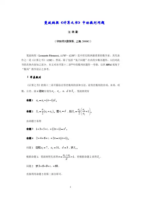
斐波纳契《计算之书》中的数列问题汪 晓 勤（华东师大数学系, 上海, 200062）斐波纳契（Leonardo Fibonacci, 1170?～1250?）是中世纪欧洲最重要的数学家，其代表作之一是《计算之书》（1202）。

然而，除了包括“兔子问题”在内的少数名题外，人们对此书的具体内容知之甚少。

本文对该书第十二章[1]中的数列问题作一考察，以供HPM 视角下“数列”教学设计之参考。

1 等差数列《计算之书》的第十二章开篇给出等差数列的求和方法。

设等差数列的首项、末项、项数、公差、前n 项和分别为1a 、n a 、n 、d 和n S 。

斐波纳契有命题1 ()11n a a n d =+-。

命题2 ()12n n n S a a =+。

若1a d =，则112n n n a a S a ⎛⎫=+ ⎪⎝⎭。

由命题2易得命题3 ()213521n n ++++-= 。

命题4 ()24621n n n ++++=+ 。

问题1 已知17a =、31n a =、3d =，求n S 。

根据命题1，斐波纳契先求得11n a a n d-=+，再根据命题2求得n S 。

问题2 求36960++++ 。

直接利用命题2的第二部分即可。

问题3 甲乙二人长途旅行，甲日行20里，乙第一日行1里，第二日行2里，第三日行3里，依此类推，日增1里。

问：二人几日后相遇？由命题2，()1202n n n +=，故斐波纳契的解法如下：20乘以2得40，从中减去1得39，此即二人相遇所需天数。

问题4 甲日行21里，乙从1里开始，日行里数按连续奇数逐日递增。

[问：几日后乙追上甲？]由命题3易得21n =。

问题5 甲日行30里，乙从2里开始，日行里数按连续偶数逐日递增。

[问：几日后乙追上甲？]由命题4易得29n =。

以下问题的解法均类似。

问题6 甲日行60里，乙第一日行3里，第二日行6里，第三天9里，等等。

[问：几日后乙追上甲？]问题7 甲日行60里，乙第一日行5里，以后日增5里。

美国数学竞赛AMC8必须掌握的常⽤单词美国数学竞赛AMC8必须掌握的常⽤单词(按字母顺序整理)⾮正态分布abnormal distribution ⾓angle平均数average 加plus（prep.）, add（v.）, addition（n.）振幅amplitude 反正弦arc sine 反余弦arc cosine 反正切arc tangent 反余切arc cotangent 反正割arc secant 反余割arc cosecant 被加数augend, summand 加数addend 轴axis 弧arc ⾯积area 算术arithmetic 公理axiom 代数algebra 锐⾓acute angle 锐⾓三⾓形acute triangle B ⼆进制binary system 折线统计图broken line graph 底base条形统计图bar graph重⼼barycentre（BrE, barycenter（AmE）C 全等congruent 曲线统计图curve diagram 进位carry 计算calculation 系数coefficient 三次⽅程cubic equation常量constant 微积分calculus 复数complex number 坐标系coordinates 组合combination 外切圆circumcircle 余割cosecant 余切cotangent 余弦cosine 圆周circumference 圆柱cylinder 圆锥cone 圆circle ⽴⽅体cube圆⼼centre（BrE）, center（AmE）D ⼩数点decimal point ⼩数decimal ⾓度degree 除divided by （prep.）, divide（v.）, division（n.）被除数dividend 除数divisor 数字digit 分母denominator ⼗进制decimal system 微分differential 导数derivative 定积分definite integral ⾏列式determinant 分布distribution ⼗⾯体decahedron ⼗⼆⾯体dodecahedron ⼗⼆边形dodecagon ⼗边形decagon 直径diameter E 等于equals, is equal to, is equivalent to 等式，⽅程式equation 等边三⾓形equilateral trian gle 外⼼excentre（BrE）, excenter（AmE）旁⼼escentre（BrE）, escenter （AmE）正多边形equilateral polygon 九⾯体enneahedron 九边形enneagon 椭圆ellipse F 分数fraction公式formula, formulae（pl.）阶乘factorial 棱台frustum of a prism 圆台frustum of a cone G ⼏何geometry 图表graph H假设hypothesis, hypotheses（pl.）⼗⼀⾯体hendecahedron 六边形hexagon 七⾯体heptahedron 半球hemisphere 六⾯体hexahedron ⼗⼀边形hendecagon 七边形heptagon ⼗六进制hexadecimal system 柱形统计图histogram ⾼height 斜边hypotenuse 双曲线hyperbola I内⼼incentre（BrE）, incenter（AmE）⼆⼗⾯体icosahedron图象imag ⽆穷⼤infinite（a.）infinity（n.）⽆穷⼩infinitesimal 积分integrale 等腰梯形isosceles trapezoid 不定积分indefinite integral 不等式inequation 整数integer ⼩于is lesser than ⼤于is greater than ⼤于等于is equal or greater than线line ⼩于等于is equal or lesser than ⽆效数字insignificant digit 相交intersect ⽆理数irrational number 虚数imaginary number 等腰三⾓形isosceles triangle 内切圆inscribed circle 极限limit 直⾓边leg 长length 轨迹locus, loca（pl.）M数学mathematics, maths（BrE）, math（AmE）被减数minuend 被乘数multiplicand, 乘数multiplicator 单项式monomial 单调性monotonicity矩阵matrix N 正态分布normal distribution 数number ⾃然数natural number 分⼦numerator 负negative 零null, zero, nought, nil O运算符operator 运算operation 钝⾓obtuse angle 钝⾓三⾓形obtuse triangle 垂⼼orthocentre（BrE）, orthocenter（AmE）原点origin ⼋⾯体octahedron⼋边形octagon P抛物线parabola 五⾯体pentahedron 平⾏六⾯体parallelepiped 相位phase周期period证明prove命题proposition 积product 正positive 多项式polynomial, multinomial 奇偶性parity 周期性periodicity点point ⾯plane 平⾏parallel 周⾓perigon平⾏四边形parallelogram 勾股定理Pythagorean theorem扇形统计图pie diagram 概率，或然率probability排列permutation ⽐例propotion 百分⽐percent百分点percentage 百分位数percentile 多⾯体polyhedron 圆周率p i 棱锥pyramid 棱柱prism 周长perimeter五边形pentagon 多边形polygon Q商quotient ⼆次⽅程quadratic equation 四次⽅程quartic equation 四边形quadrilateral R直⾓梯形right trapezoid 标准差root-mean-square deviation, standard deviation 差remainder⽐ratio 四舍五⼊round 下舍⼊round down 上舍⼊round up 值域range 有理数rational number 实数real number 直⾓right angle 射线radial 弧度radian 直⾓三⾓形right triangle 矩形rectangle 旋转rotation 菱形rhomb, rhombus, rhombi（pl.）,diamond 环ring 半径radius S正⽅形square 有效数字significant digit ⼀次⽅程simple equation 体solid 线段segment 平⾓straight angle 边side不等边三⾓形scalene triangle 空间space 球sphere 正弦sine 统计statistics 和sum 减minus（prep.）, subtract（v.）, subtraction （n.）减数subtrahend 数列，级数series 正割secant表⾯积surface area 相似similar半圆semicircle 扇形sector T梯形trapezoid 截尾truncation 定理theorem乘times（prep.）, multiply（v.）, multiplication（n.）faciend三⾓形triangle 正切tangent 三⾓trigonometry四⾯体tetrahedron U未知数unknown, x-factor, y-factor, z-factor 底⾯undersurface 变量variable⽅差variance 体积volume W 权weight, significance宽width 加权平均数weighted average X 坐标轴x-axis, y-axis, z-axis 横坐标x-coordinate 纵坐标y-coordinate数学mathematics, maths（BrE）, math（AmE）被除数dividend除数divisor 商quotient 等于equals, is equal to, is equivalent to ⼤于is greater than ⼩于is lesser than ⼤于等于is equal or greater than ⼩于等于is equal or lesser than 运算符operator数字digit 数number ⾃然数natural number 公理axiom定理theorem 计算calculation 运算operation 证明prove假设hypothesis, hypotheses（pl.）命题proposition 算术arithmetic 加plus（prep.）, add（v.）, addition（n.）被加数augend, summand 加数addend 和sum 减minus（prep.）, subtract（v.）, subtraction（n.）被减数minuend 减数subtrahend 差remainder 乘times（prep.）, multiply（v.）, multiplication（n.）被乘数multiplicand, faciend 乘数multiplicator 积product除divided by（prep.）, divide（v.）, division（n.）整数integer⼩数decimal ⼩数点decimal point 分数fraction分⼦numerator 分母denominator ⽐ratio正positive 负negative 零null, zero, nought, nil⼗进制decimal system ⼆进制binary system ⼗六进制hexadecimal system 权weight, significance进位carry 截尾truncation 四舍五⼊round下舍⼊round down 上舍⼊round up有效数字significant digit ⽆效数字insignificant digit代数algebra 公式formula, formulae（pl.）单项式monomial多项式polynomial, multinomial 系数coefficient未知数unknown, x-factor, y-factor, z-factor 等式，⽅程式equation⼀次⽅程simple equation ⼆次⽅程quadratic equation 三次⽅程cubic equation 四次⽅程quartic equation 不等式inequation阶乘factorial 对数logarithm 指数，幂exponent 乘⽅power⼆次⽅，平⽅square 三次⽅，⽴⽅cube 四次⽅the power of four, the fourth power n次⽅the power of n, the nth power开⽅evolution, extraction ⼆次⽅根，平⽅根square root三次⽅根，⽴⽅根cube root 四次⽅根the root of four, the fourth root n次⽅根the root of n, the nth root 集合aggregate元素element 空集void ⼦集subset 交集intersection 并集union 补集complement 映射mapping 函数function 定义域domain, field of definition 值域range 常量constant变量variable 单调性monotonicity 奇偶性parity周期性periodicity 图象image 数列，级数series 微积分calculus微分differential 导数derivative 极限limit⽆穷⼤infinite（a.）infinity（n.）⽆穷⼩infinitesimal积分integral 定积分definite integral不定积分indefinite integral 有理数rational number⽆理数irrational number 实数real number虚数imaginary number 复数complex number 矩阵matrix⾏列式determinant ⼏何geometry 点point 线line ⾯plane 体solid 线段segment 射线radial平⾏parallel 相交intersect ⾓angle ⾓度degree 弧度radian锐⾓acute angle 直⾓right angle 钝⾓obtuse angle 平⾓straight angle 周⾓perigon 底base 边side ⾼height 三⾓形triangle锐⾓三⾓形acute triangle 直⾓三⾓形right triangle 直⾓边leg斜边hypotenuse 勾股定理Pythagorean theorem 钝⾓三⾓形obtuse triangle 不等边三⾓形scalene triangle 等腰三⾓形isosceles triangle 等边三⾓形equilateral triangle 四边形quadrilateral平⾏四边形parallelogram 矩形rectangle长length 宽width 菱形rhomb, rhombus, rhombi（pl.）, diamond正⽅形square 梯形trapezoid 直⾓梯形right trapezoid等腰梯形isosceles trapezoid 五边形pentagon 六边形hexagon 七边形heptagon ⼋边形octagon 九边形enneagon⼗边形decagon ⼗⼀边形hendecagon ⼗⼆边形dodecagon 多边形polygon 正多边形equilateral polygon 圆circle圆⼼centre（BrE）, center（AmE）半径radius 直径diameter 圆周率pi 弧arc半圆semicircle 扇形sector 环ring 椭圆ellipse 圆周circumference 周长perimeter ⾯积area 轨迹locus, loca（pl.）相似similar 全等congruent 四⾯体tetrahedron 五⾯体pentahedron六⾯体hexahedron 平⾏六⾯体parallelepiped ⽴⽅体cube 七⾯体heptahedron ⼋⾯体octahedron 九⾯体enneahedron ⼗⾯体decahedron⼗⼀⾯体hendecahedron ⼗⼆⾯体dodecahedron ⼆⼗⾯体icosahedron多⾯体polyhedron 棱锥pyramid 棱柱prism 棱台frustum of a prism旋转rotation 轴axis 圆锥cone 圆柱cylinder 圆台frustum of a cone 球sphere 半球hemisphere 底⾯undersurface 表⾯积surface area 体积volume 空间space 坐标系coordinates 坐标轴x-axis,y-axis, z-axis 横坐标x-coordinate 纵坐标y-coordinate原点origin 双曲线hyperbola 抛物线parabola 三⾓trigonometry 正弦sine 余弦cosine 正切tangent 余切cotangent 正割secant 余割cosecant 反正弦arc sine 反余弦arc cosine 反正切arc tangent 反余切arc cotangent 反正割arc secant 反余割arc cosecant 相位phase 周期period 振幅amplitude 内⼼incentre（BrE）, incenter （AmE）外⼼excentre（BrE）, excenter（AmE）旁⼼escentre（BrE）, escenter （AmE）垂⼼orthocentre（BrE）,orthocenter（AmE）重⼼barycentre （BrE）, barycenter（AmE）内切圆inscribed circle 外切圆circumcircle 统计statistics 平均数average 加权平均数weighted average⽅差variance 标准差root-mean-square deviation, standard deviation ⽐例propotion 百分⽐percent 百分点percentage 百分位数percentile 排列permutation 组合combination 概率，或然率probability 分布distribution 正态分布normal distribution⾮正态分布abnormal distribution 图表graph 条形统计图bar graph 柱形统计图histogram 折线统计图broken line graph 曲线统计图curve diagram。

Proceedings of the IASTED International ConferenceParallel and Distributed Computing and SystemsNovember3-6,1999,MIT,Boston,USAParallel Refinement of Unstructured MeshesJos´e G.Casta˜n os and John E.SavageDepartment of Computer ScienceBrown UniversityE-mail:jgc,jes@AbstractIn this paper we describe a parallel-refinement al-gorithm for unstructuredfinite element meshes based on the longest-edge bisection of triangles and tetrahedrons. This algorithm is implemented in P ARED,a system that supports the parallel adaptive solution of PDEs.We dis-cuss the design of such an algorithm for distributed mem-ory machines including the problem of propagating refine-ment across processor boundaries to obtain meshes that are conforming and non-degenerate.We also demonstrate that the meshes obtained by this algorithm are equivalent to the ones obtained using the serial longest-edge refine-ment method.Wefinally report on the performance of this refinement algorithm on a network of workstations.Keywords:mesh refinement,unstructured meshes,finite element methods,adaptation.1.IntroductionThefinite element method(FEM)is a powerful and successful technique for the numerical solution of partial differential equations.When applied to problems that ex-hibit highly localized or moving physical phenomena,such as occurs on the study of turbulence influidflows,it is de-sirable to compute their solutions adaptively.In such cases, adaptive computation has the potential to significantly im-prove the quality of the numerical simulations by focusing the available computational resources on regions of high relative error.Unfortunately,the complexity of algorithms and soft-ware for mesh adaptation in a parallel or distributed en-vironment is significantly greater than that it is for non-adaptive computations.Because a portion of the given mesh and its corresponding equations and unknowns is as-signed to each processor,the refinement(coarsening)of a mesh element might cause the refinement(coarsening)of adjacent elements some of which might be in neighboring processors.To maintain approximately the same number of elements and vertices on every processor a mesh must be dynamically repartitioned after it is refined and portions of the mesh migrated between processors to balance the work.In this paper we discuss a method for the paral-lel refinement of two-and three-dimensional unstructured meshes.Our refinement method is based on Rivara’s serial bisection algorithm[1,2,3]in which a triangle or tetrahe-dron is bisected by its longest edge.Alternative efforts to parallelize this algorithm for two-dimensional meshes by Jones and Plassman[4]use randomized heuristics to refine adjacent elements located in different processors.The parallel mesh refinement algorithm discussed in this paper has been implemented as part of P ARED[5,6,7], an object oriented system for the parallel adaptive solu-tion of partial differential equations that we have devel-oped.P ARED provides a variety of solvers,handles selec-tive mesh refinement and coarsening,mesh repartitioning for load balancing,and interprocessor mesh migration.2.Adaptive Mesh RefinementIn thefinite element method a given domain is di-vided into a set of non-overlapping elements such as tri-angles or quadrilaterals in2D and tetrahedrons or hexahe-drons in3D.The set of elements and its as-sociated vertices form a mesh.With theaddition of boundary conditions,a set of linear equations is then constructed and solved.In this paper we concentrate on the refinement of conforming unstructured meshes com-posed of triangles or tetrahedrons.On unstructured meshes, a vertex can have a varying number of elements adjacent to it.Unstructured meshes are well suited to modeling do-mains that have complex geometry.A mesh is said to be conforming if the triangles and tetrahedrons intersect only at their shared vertices,edges or faces.The FEM can also be applied to non-conforming meshes,but conformality is a property that greatly simplifies the method.It is also as-sumed to be a requirement in this paper.The rate of convergence and quality of the solutions provided by the FEM depends heavily on the number,size and shape of the mesh elements.The condition number(a)(b)(c)Figure1:The refinement of the mesh in using a nested refinement algorithm creates a forest of trees as shown in and.The dotted lines identify the leaf triangles.of the matrices used in the FEM and the approximation error are related to the minimum and maximum angle of all the elements in the mesh[8].In three dimensions,the solid angle of all tetrahedrons and their ratio of the radius of the circumsphere to the inscribed sphere(which implies a bounded minimum angle)are usually used as measures of the quality of the mesh[9,10].A mesh is non-degenerate if its interior angles are never too small or too large.For a given shape,the approximation error increases with ele-ment size(),which is usually measured by the length of the longest edge of an element.The goal of adaptive computation is to optimize the computational resources used in the simulation.This goal can be achieved by refining a mesh to increase its resolution on regions of high relative error in static problems or by re-fining and coarsening the mesh to follow physical anoma-lies in transient problems[11].The adaptation of the mesh can be performed by changing the order of the polynomi-als used in the approximation(-refinement),by modifying the structure of the mesh(-refinement),or a combination of both(-refinement).Although it is possible to replace an old mesh with a new one with smaller elements,most -refinement algorithms divide each element in a selected set of elements from the current mesh into two or more nested subelements.In P ARED,when an element is refined,it does not get destroyed.Instead,the refined element inserts itself into a tree,where the root of each tree is an element in the initial mesh and the leaves of the trees are the unrefined elements as illustrated in Figure1.Therefore,the refined mesh forms a forest of refinement trees.These trees are used in many of our algorithms.Error estimates are used to determine regions where adaptation is necessary.These estimates are obtained from previously computed solutions of the system of equations. After adaptation imbalances may result in the work as-signed to processors in a parallel or distributed environ-ment.Efficient use of resources may require that elements and vertices be reassigned to processors at runtime.There-fore,any such system for the parallel adaptive solution of PDEs must integrate subsystems for solving equations,adapting a mesh,finding a good assignment of work to processors,migrating portions of a mesh according to anew assignment,and handling interprocessor communica-tion efficiently.3.P ARED:An OverviewP ARED is a system of the kind described in the lastparagraph.It provides a number of standard iterativesolvers such as Conjugate Gradient and GMRES and pre-conditioned versions thereof.It also provides both-and -refinement of meshes,algorithms for adaptation,graph repartitioning using standard techniques[12]and our ownParallel Nested Repartitioning(PNR)[7,13],and work mi-gration.P ARED runs on distributed memory parallel comput-ers such as the IBM SP-2and networks of workstations.These machines consist of coarse-grained nodes connectedthrough a high to moderate latency network.Each nodecannot directly address a memory location in another node. In P ARED nodes exchange messages using MPI(Message Passing Interface)[14,15,16].Because each message has a high startup cost,efficient message passing algorithms must minimize the number of messages delivered.Thus, it is better to send a few large messages rather than many small ones.This is a very important constraint and has a significant impact on the design of message passing algo-rithms.P ARED can be run interactively(so that the user canvisualize the changes in the mesh that results from meshadaptation,partitioning and migration)or without directintervention from the user.The user controls the systemthrough a GUI in a distinguished node called the coordina-tor,.This node collects information from all the other processors(such as its elements and vertices).This tool uses OpenGL[17]to permit the user to view3D meshes from different angles.Through the coordinator,the user can also give instructions to all processors such as specify-ing when and how to adapt the mesh or which strategy to use when repartitioning the mesh.In our computation,we assume that an initial coarse mesh is given and that it is loaded into the coordinator.The initial mesh can then be partitioned using one of a num-ber of serial graph partitioning algorithms and distributed between the processors.P ARED then starts the simulation. Based on some adaptation criterion[18],P ARED adapts the mesh using the algorithms explained in Section5.Af-ter the adaptation phase,P ARED determines if a workload imbalance exists due to increases and decreases in the num-ber of mesh elements on individual processors.If so,it invokes a procedure to decide how to repartition mesh el-ements between processors;and then moves the elements and vertices.We have found that PNR gives partitions with a quality comparable to those provided by standard meth-ods such as Recursive Spectral Bisection[19]but which(b)(a)Figure2:Mesh representation in a distributed memory ma-chine using remote references.handles much larger problems than can be handled by stan-dard methods.3.1.Object-Oriented Mesh RepresentationsIn P ARED every element of the mesh is assigned to a unique processor.V ertices are shared between two or more processors if they lie on a boundary between parti-tions.Each of these processors has a copy of the shared vertices and vertices refer to each other using remote ref-erences,a concept used in object-oriented programming. This is illustrated in Figure2on which the remote refer-ences(marked with dashed arrows)are used to maintain the consistency of multiple copies of the same vertex in differ-ent processors.Remote references are functionally similar to standard C pointers but they address objects in a different address space.A processor can use remote references to invoke meth-ods on objects located in a different processor.In this case, the method invocations and arguments destined to remote processors are marshalled into messages that contain the memory addresses of the remote objects.In the destina-tion processors these addresses are converted to pointers to objects of the corresponding type through which the meth-ods are invoked.Because the different nodes are inher-ently trusted and MPI guarantees reliable communication, P ARED does not incur the overhead traditionally associated with distributed object systems.Another idea commonly found in object oriented pro-gramming and which is used in P ARED is that of smart pointers.An object can be destroyed when there are no more references to it.In P ARED vertices are shared be-tween several elements and each vertex counts the number of elements referring to it.When an element is created, the reference count of its vertices is incremented.Simi-larly,when the element is destroyed,the reference count of its vertices is decremented.When the reference count of a vertex reaches zero,the vertex is no longer attached to any element located in the processor and can be destroyed.If a vertex is shared,then some other processor might have a re-mote reference to it.In that case,before a copy of a shared vertex is destroyed,it informs the copies in other processors to delete their references to itself.This procedure insures that the shared vertex can then be safely destroyed without leaving dangerous dangling pointers referring to it in other processors.Smart pointers and remote references provide a simple replication mechanism that is tightly integrated with our mesh data structures.In adaptive computation,the struc-ture of the mesh evolves during the computation.During the adaptation phase,elements and vertices are created and destroyed.They may also be assigned to a different pro-cessor to rebalance the work.As explained above,remote references and smart pointers greatly simplify the task of creating dynamic meshes.4.Adaptation Using the Longest Edge Bisec-tion AlgorithmMany-refinement techniques[20,21,22]have been proposed to serially refine triangular and tetrahedral meshes.One widely used method is the longest-edge bisec-tion algorithm proposed by Rivara[1,2].This is a recursive procedure(see Figure3)that in two dimensions splits each triangle from a selected set of triangles by adding an edge between the midpoint of its longest side to the opposite vertex.In the case that makes a neighboring triangle,,non-conforming,then is refined using the same algorithm.This may cause the refinement to prop-agate throughout the mesh.Nevertheless,this procedure is guaranteed to terminate because the edges it bisects in-crease in length.Building on the work of Rosenberg and Stenger[23]on bisection of triangles,Rivara[1,2]shows that this refinement procedure provably produces two di-mensional meshes in which the smallest angle of the re-fined mesh is no less than half of the smallest angle of the original mesh.The longest-edge bisection algorithm can be general-ized to three dimensions[3]where a tetrahedron is bisected into two tetrahedrons by inserting a triangle between the midpoint of its longest edge and the two vertices not in-cluded in this edge.The refinement propagates to neigh-boring tetrahedrons in a similar way.This procedure is also guaranteed to terminate,but unlike the two dimensional case,there is no known bound on the size of the small-est angle.Nevertheless,experiments conducted by Rivara [3]suggest that this method does not produce degenerate meshes.In two dimensions there are several variations on the algorithm.For example a triangle can initially be bisected by the longest edge,but then its children are bisected by the non-conforming edge,even if it is that is not their longest edge[1].In three dimensions,the bisection is always per-formed by the longest edge so that matching faces in neigh-boring tetrahedrons are always bisected by the same com-mon edge.Bisect()let,and be vertices of the trianglelet be the longest side of and let be the midpoint ofbisect by the edge,generating two new triangles andwhile is a non-conforming vertex dofind the non-conforming triangle adjacent to the edgeBisect()end whileFigure3:Longest edge(Rivara)bisection algorithm for triangular meshes.Because in P ARED refined elements are not destroyed in the refinement tree,the mesh can be coarsened by replac-ing all the children of an element by their parent.If a parent element is selected for coarsening,it is important that all the elements that are adjacent to the longest edge of are also selected for coarsening.If neighbors are located in different processors then only a simple message exchange is necessary.This algorithm generates conforming meshes: a vertex is removed only if all the elements that contain that vertex are all coarsened.It does not propagate like the re-finement algorithm and it is much simpler to implement in parallel.For this reason,in the rest of the paper we will focus on the refinement of meshes.5.Parallel Longest-Edge RefinementThe longest-edge bisection algorithm and many other mesh refinement algorithms that propagate the refinement to guarantee conformality of the mesh are not local.The refinement of one particular triangle or tetrahedron can propagate through the mesh and potentially cause changes in regions far removed from.If neighboring elements are located in different processors,it is necessary to prop-agate this refinement across processor boundaries to main-tain the conformality of the mesh.In our parallel longest edge bisection algorithm each processor iterates between a serial phase,in which there is no communication,and a parallel phase,in which each processor sends and receives messages from other proces-sors.In the serial phase,processor selects a setof its elements for refinement and refines them using the serial longest edge bisection algorithms outlined earlier. The refinement often creates shared vertices in the bound-ary between adjacent processors.To minimize the number of messages exchanged between and,delays the propagation of refinement to until has refined all the elements in.The serial phase terminates when has no more elements to refine.A processor informs an adjacent processor that some of its elements need to be refined by sending a mes-sage from to containing the non-conforming edges and the vertices to be inserted at their midpoint.Each edge is identified by its endpoints and and its remote ref-erences(see Figure4).If and are sharedvertices,(a)(c)(b)Figure4:In the parallel longest edge bisection algo-rithm some elements(shaded)are initially selected for re-finement.If the refinement creates a new(black)ver-tex on a processor boundary,the refinement propagates to neighbors.Finally the references are updated accord-ingly.then has a remote reference to copies of and lo-cated in processor.These references are included in the message,so that can identify the non-conforming edge and insert the new vertex.A similar strategy can be used when the edge is refined several times during the re-finement phase,but in this case,the vertex is not located at the midpoint of.Different processors can be in different phases during the refinement.For example,at any given time a processor can be refining some of its elements(serial phase)while neighboring processors have refined all their elements and are waiting for propagation messages(parallel phase)from adjacent processors.waits until it has no elements to refine before receiving a message from.For every non-conforming edge included in a message to,creates its shared copy of the midpoint(unless it already exists) and inserts the new non-conforming elements adjacent to into a new set of elements to be refined.The copy of in must also have a remote reference to the copy of in.For this reason,when propagates the refine-ment to it also includes in the message a reference to its copies of shared vertices.These steps are illustrated in Figure4.then enters the serial phase again,where the elements in are refined.(c)(b)(a)Figure5:Both processors select(shaded)mesh el-ements for refinement.The refinement propagates to a neighboring processor resulting in more elements be-ing refined.5.1.The Challenge of Refining in ParallelThe description of the parallel refinement algorithm is not complete because refinement propagation across pro-cessor boundaries can create two synchronization prob-lems.Thefirst problem,adaptation collision,occurs when two(or more)processors decide to refine adjacent elements (one in each processor)during the serial phase,creating two(or more)vertex copies over a shared edge,one in each processor.It is important that all copies refer to the same logical vertex because in a numerical simulation each ver-tex must include the contribution of all the elements around it(see Figure5).The second problem that arises,termination detection, is the determination that a refinement phase is complete. The serial refinement algorithm terminates when the pro-cessor has no more elements to refine.In the parallel ver-sion termination is a global decision that cannot be deter-mined by an individual processor and requires a collabora-tive effort of all the processors involved in the refinement. Although a processor may have adapted all of its mesh elements in,it cannot determine whether this condition holds for all other processors.For example,at any given time,no processor might have any more elements to re-fine.Nevertheless,the refinement cannot terminate because there might be some propagation messages in transit.The algorithm for detecting the termination of parallel refinement is based on Dijkstra’s general distributed termi-nation algorithm[24,25].A global termination condition is reached when no element is selected for refinement.Hence if is the set of all elements in the mesh currently marked for refinement,then the algorithmfinishes when.The termination detection procedure uses message ac-knowledgments.For every propagation message that receives,it maintains the identity of its source()and to which processors it propagated refinements.Each prop-agation message is acknowledged.acknowledges to after it has refined all the non-conforming elements created by’s message and has also received acknowledgments from all the processors to which it propagated refinements.A processor can be in two states:an inactive state is one in which has no elements to refine(it cannot send new propagation messages to other processors)but can re-ceive messages.If receives a propagation message from a neighboring processor,it moves from an inactive state to an active state,selects the elements for refinement as spec-ified in the message and proceeds to refine them.Let be the set of elements in needing refinement.A processor becomes inactive when:has received an acknowledgment for every propa-gation message it has sent.has acknowledged every propagation message it has received..Using this definition,a processor might have no more elements to refine()but it might still be in an active state waiting for acknowledgments from adjacent processors.When a processor becomes inactive,sends an acknowledgment to the processors whose propagation message caused to move from an inactive state to an active state.We assume that the refinement is started by the coordi-nator processor,.At this stage,is in the active state while all the processors are in the inactive state.ini-tiates the refinement by sending the appropriate messages to other processors.This message also specifies the adapta-tion criterion to use to select the elements for refinement in.When a processor receives a message from,it changes to an active state,selects some elements for refine-ment either explicitly or by using the specified adaptation criterion,and then refines them using the serial bisection algorithm,keeping track of the vertices created over shared edges as described earlier.When itfinishes refining its ele-ments,sends a message to each processor on whose shared edges created a shared vertex.then listens for messages.Only when has refined all the elements specified by and is not waiting for any acknowledgment message from other processors does it sends an acknowledgment to .Global termination is detected when the coordinator becomes inactive.When receives an acknowledgment from every processor this implies that no processor is re-fining an element and that no processor is waiting for an acknowledgment.Hence it is safe to terminate the refine-ment.then broadcasts this fact to all the other proces-sors.6.Properties of Meshes Refined in ParallelOur parallel refinement algorithm is guaranteed to ter-minate.In every serial phase the longest edge bisectionLet be a set of elements to be refinedwhile there is an element dobisect by its longest edgeinsert any non-conforming element intoend whileFigure6:General longest-edge bisection(GLB)algorithm.algorithm is used.In this algorithm the refinement prop-agates towards progressively longer edges and will even-tually reach the longest edge in each processor.Between processors the refinement also propagates towards longer edges.Global termination is detected by using the global termination detection procedure described in the previous section.The resulting mesh is conforming.Every time a new vertex is created over a shared edge,the refinement propagates to adjacent processors.Because every element is always bisected by its longest edge,for triangular meshes the results by Rosenberg and Stenger on the size of the min-imum angle of two-dimensional meshes also hold.It is not immediately obvious if the resulting meshes obtained by the serial and parallel longest edge bisection al-gorithms are the same or if different partitions of the mesh generate the same refined mesh.As we mentioned earlier, messages can arrive from different sources in different or-ders and elements may be selected for refinement in differ-ent sequences.We now show that the meshes that result from refining a set of elements from a given mesh using the serial and parallel algorithms described in Sections4and5,re-spectively,are the same.In this proof we use the general longest-edge bisection(GLB)algorithm outlined in Figure 6where the order in which elements are refined is not spec-ified.In a parallel environment,this order depends on the partition of the mesh between processors.After showing that the resulting refined mesh is independent of the order in which the elements are refined using the serial GLB al-gorithm,we show that every possible distribution of ele-ments between processors and every order of parallel re-finement yields the same mesh as would be produced by the serial algorithm.Theorem6.1The mesh that results from the refinement of a selected set of elements of a given mesh using the GLB algorithm is independent of the order in which the elements are refined.Proof:An element is refined using the GLBalgorithm if it is in the initial set or refinementpropagates to it.An element is refinedif one of its neighbors creates a non-conformingvertex at the midpoint of one of its edges.Therefinement of by its longest edge divides theelement into two nested subelements andcalled the children of.These children are inturn refined by their longest edge if one of their edges is non-conforming.The refinement proce-dure creates a forest of trees of nested elements where the root of each tree is an element in theinitial mesh and the leaves are unrefined ele-ments.For every element,let be the refinement tree of nested elements rooted atwhen the refinement procedure terminates. Using the GLB procedure elements can be se-lected for refinement in different orders,creating possible different refinement histories.To show that this cannot happen we assume the converse, namely,that two refinement histories and generate different refined meshes,and establish a contradiction.Thus,assume that there is an ele-ment such that the refinement trees and,associated with the refinement histories and of respectively,are different.Be-cause the root of and is the same in both refinement histories,there is a place where both treesfirst differ.That is,starting at the root,there is an element that is common to both trees but for some reason,its children are different.Be-cause is always bisected by the longest edge, the children of are different only when is refined in one refinement history and it is not re-fined in the other.In other words,in only one of the histories does have children.Because is refined in only one refinement his-tory,then,the initial set of elements to refine.This implies that must have been refined because one of its edges became non-conforming during one of the refinement histo-ries.Let be the set of elements that are present in both refinement histories,but are re-fined in and not in.We define in a similar way.For each refinement history,every time an ele-ment is refined,it is assigned an increasing num-ber.Select an element from either or that has the lowest number.Assume that we choose from so that is refined in but not in.In,is refined because a neigh-boring element created a non-conforming ver-tex at the midpoint of their shared edge.There-fore is refined in but not in because otherwise it would cause to be refined in both sequences.This implies that is also in and has a lower refinement number than con-。

11
iv
⌂
CONTENTS OF SECTION 1
☰ Hydraulics
⌂ Cameron Hydraulic Data ☰
Introduction. . . . . . . . . . . . . ................................................................ 1-3 Liquids. . . . . . . . . . . . . . . . . . . ...................................... .......................... 1-3
4
Viscosity etc.
Steam data....................................................................................................................................................................................... 6
1 Liquid Flow.............................................................................. 1-4
Viscosity. . . . . . . . . . . . . . . . . ...................................... .......................... 1-5 Pumping. . . . . . . . . . . . . . . . . ...................................... .......................... 1-6 Volume-System Head Calculations-Suction Head. ........................... 1-6, 1-7 Suction Lift-Total Discharge Head-Velocity Head............................. 1-7, 1-8 Total Sys. Head-Pump Head-Pressure-Spec. Gravity. ...................... 1-9, 1-10 Net Positive Suction Head. .......................................................... 1-11 NPSH-Suction Head-Life; Examples:....................... ............... 1-11 to 1-16 NPSH-Hydrocarbon Corrections.................................................... 1-16 NPSH-Reciprocating Pumps. ....................................................... 1-17 Acceleration Head-Reciprocating Pumps. ........................................ 1-18 Entrance Losses-Specific Speed. .................................................. 1-19 Specific Speed-Impeller. .................................... ........................ 1-19 Specific Speed-Suction...................................... ................. 1-20, 1-21 Submergence.. . . . . . . . . ....................................... ................. 1-21, 1-22 Intake Design-Vertical Wet Pit Pumps....................................... 1-22, 1-27 Work Performed in Pumping. ............................... ........................ 1-27 Temperature Rise. . . . . . . ...................................... ........................ 1-28 Characteristic Curves. . ...................................... ........................ 1-29 Affinity Laws-Stepping Curves. ..................................................... 1-30 System Curves.. . . . . . . . ....................................... ........................ 1-31 Parallel and Series Operation. .............................. ................. 1-32, 1-33 Water Hammer. . . . . . . . . . ...................................... ........................ 1-34 Reciprocating Pumps-Performance. ............................................... 1-35 Recip. Pumps-Pulsation Analysis & System Piping...................... 1-36 to 1-45 Pump Drivers-Speed Torque Curves. ....................................... 1-45, 1-46 Engine Drivers-Impeller Profiles. ................................................... 1-47 Hydraulic Institute Charts.................................... ............... 1-48 to 1-52 Bibliography.. . . . . . . . . . . . ...................................... ........................ 1-53

1795年高斯进入 HYPERLINK 哥廷根大学 。1796年，19岁的高斯得到了一个数 学史上极重要的结果，就是《正十七边形尺规作图之理论与方法》。1798年转入黑 尔姆施泰特大学，翌年因证明代数基本定理获博士学位。
1801年， HYPERLINK 高斯 又证明了形如"Fermat素数"边数的正多边形可以由 尺规作出。
1796年，约翰 卡尔 弗里德里希 高斯证明了可以尺规作正十七边形。1807年高斯成 为 HYPERLINK blank" 哥廷根 大学教授和哥廷根天文台台长。1818年—1826年 间， HYPERLINK
汉诺威 公国的大地测量工作由 HYPERLINK
高斯 主导。1840年高斯与韦伯一同画出世界上第一张地球磁场图。
数学家高斯（课堂PPT）
演讲人
约翰 卡尔 弗里德里希 高斯（Johann Carl Friedrich Gauß），男，1777年4月30日 出生于不伦瑞克，德国著名数学家、物理学家、天文学家、几何学家， HYPERLINK blank" 大地测量 学家，
毕业于Carolinum学院（现 HYPERLINK blank" 布伦瑞克工业大学 ），也 就是众人熟识的高斯，与欧拉并称数学史上两大巨星。
约翰 卡尔 弗里德里希 高斯（1777年4月30日—1855年2月23日），生 于不伦瑞克，卒于哥廷根，哥廷根学派的先驱之一。
约翰 卡尔 弗里德里希 高斯的成就遍布于数学的各个领域，在内蕴几何、数论、双 曲几何、微分几何、超几何级数、复分析以及椭圆分析等方面均有开创性贡献。他 十分注重数学的应用，并且在对天文学、 HYPERLINK " 大地测量学 和磁学的研究 中也偏重于用数学方法进行研究。

Divide and Conquer当输入数据的规模很小时，比如只有一个或两个数字，则绝大多数的问题都很容易解。

可是当输入规模增大时，问题往往变得很难。

因此，算法设计的一个基本方法就是寻找大规模问题解与小规摸问题解之间的关系。

分治术(Divide and Conquer)是这种方法之一。

后面要讲的贪心法和动态规划也是基于这种方法但技巧上有不同之处。

简单地说，分治术的做法是将一个规模为n的问题分解为整数个规模小些的子问题，然后找出这些子问题或者一部分子问题的解并由此得到原问题的解。

在解决这些子问题时，分治术要求用同样的方法递归解出。

那就是说，我们必须把这些子问题再分为更小的问题直至问题的规模小到可以直接解出。

这个不断分解的过程看起来很复杂，但用递归的算法表达出来却往往简洁明了。

通常，在用分治术的算法中只要讲明三件事：(1)底(bottom case)：对足够小的输入规模，如何直接解出。

(2)分(divide)：如何将一个规模为n的输入分为整数个规模小些的子问题。

(3)合(conquer) ：如何从子问题的解中获得原规模为n的解。

下面我们看一个例子。

1第一个例子−二元搜索假定有一个已排好序的数组A[1] ≤A[2] ≤…≤A[n]。

现在我们要在这n个数字中查找是否有一个数等于要找的数x。

如果是A[i] = x, 则报告序号i，否则报告无(nil)。

我们可以用以下的算法。

输入：A[p], A[p+1], …, A[r], x输出: i如果A[i] = x否则nil。

BinarySearch (A, p, r, x);1. if p > r2. then return (nil)3. midpoint ←⎣(p+r)/2⎦4. if A[midpoint] = x5. then return (midpoint)6. else if x < A[midpoint]7. then BinarySearch (A, p, midpoint-1, x)8. else BinarySearch (A, midpoint+1, r, x)9. End注意，上面的算法只是一个子程序，要搜索数组A[1], A[2], …, A[n]时，主程序需要调用BinarySearch(A, 1, n, x)。

Grünwald—Wang 定理是数论领域内一个具有重要价值的理论定理，该定理涉及了代数数论及复数域的相关问题。

Grünwald—Wang 定理最初由Grünwald 在1913年提出，后来在数论家 Wang 对其进行了深入研究并进行了重大的改进。

该定理在数论领域内引起了广泛关注，受到了学术界的高度重视。

在进行正式的介绍之前，我们首先需要了解一些基本概念。

代数数论是数论与代数学的交叉领域，研究了数论中与代数相关的问题，而复数域则是指数学中的一个概念，表示了所有实数及虚数的集合，在代数数论及复数域的研究中，一直以来都存在着一些复杂的难题，为了解决这些难题，Grünwald—Wang 定理的提出具有非常重要的意义。

接下来，我将从几个方面对Grünwald—Wang 定理进行详细的介绍：1. 定理描述Grünwald—Wang 定理是一个旨在寻找复数域中代数数的表达形式的定理。

其核心思想是，对于复数域中的任意一个代数数，都可以在复数域的有限扩张中找到一个具有一定特定性质的子域。

这个子域的存在使得复数域中的代数数可以通过一定的方式来表达，从而为复数域及其代数元素的研究提供了有力的工具。

2. 定理意义Grünwald—Wang 定理的提出填补了数论与复数域交叉领域中的空白，为代数数的表达提供了丰富多样的可能性，同时也为研究代数数的性质提供了更为宽广的视角。

通过该定理，我们可以更加深入地理解复数域及其代数元素的内在结构，为解决相关问题提供了有力的支持。

3. 研究现状Grünwald—Wang 定理的提出为相关领域的研究带来了新的思路和方法，目前，该定理被广泛应用于数论、代数学及复数域研究的一些重要问题中。

在国际学术界，Grünwald—Wang 定理的相关研究成果也层出不穷，一系列深入的推广和应用正在逐步完善与推进行中。

presburger算术自然数【原创版】目录1.Presburger 算术的概述2.Presburger 算术与自然数的关系3.Presburger 算术的应用领域正文【1.Presburger 算术的概述】Presburger 算术是一种基于自然数的算术系统，由匈牙利数学家Mojzesz Presburger 于 20 世纪初提出。

这种算术系统的主要特点是，它只允许使用加法和乘法两种运算，而不包括减法和除法。

在 Presburger 算术中，自然数被认为是基本的计算对象，通过加法和乘法运算，可以得到任意一个大于零的自然数。

【2.Presburger 算术与自然数的关系】Presburger 算术与自然数密切相关，因为它是一种基于自然数的算术系统。

在 Presburger 算术中，自然数是基本的计算对象，所有的运算都基于自然数进行。

通过 Presburger 算术，我们可以更直观地理解自然数的性质和规律。

例如，我们可以通过 Presburger 算术证明，对于任意一个大于 1 的自然数 n，总存在至少一个自然数 m，使得 m 的 n 次方大于 n。

【3.Presburger 算术的应用领域】虽然 Presburger 算术在现代数学中并不常用，但它在某些特定领域中仍然具有重要的应用价值。

例如，在计算机科学中，Presburger 算术可以用来设计一些高效的算法，用于解决一些涉及自然数的问题。

此外，Presburger 算术还可以应用于逻辑学和组合数学等领域，为这些领域提供一些新的研究方法和思路。

总之，Presburger 算术是一种基于自然数的算术系统，虽然现代数学中并不常用，但在计算机科学、逻辑学和组合数学等领域中仍具有重要的应用价值。

presburger算术自然数
**Presburger算术的概述**
Presburger算术是一种计算模型，主要用于描述和解决自然数和整数之间的数学问题。

它的命名源于数学家Jozef Presburger，他在1929年提出了一种称为"Presburger算术"的数学理论。

这个理论在当时引起了很大的关注，因为它是第一个公理化体系，能够描述自然数的性质和运算，而且比传统的皮亚诺算术更为简洁。

**Presburger算术与自然数的关系**
自然数是数学中最基本的计数概念，从0开始，依次为0，1，2，3……。

Presburger算术研究的就是这些自然数的性质和运算。

在这个体系中，自然数的概念被分为两个部分：平凡数（0和1）和非平凡数（2到无穷大）。

Presburger算术利用公理和规则来描述自然数的结构和运算，包括加法、减法、乘法、除法等。

**Presburger算术的应用领域**
Presburger算术在计算机科学、逻辑学、数学等领域具有广泛的应用。

在计算机科学中，Presburger算术被用于研究程序设计、编译器和计算机体系结构等。

在逻辑学中，Presburger算术为逻辑推理和证明提供了基础。

在数学领域，Presburger算术为研究自然数和整数的性质提供了理论支持。

**总结**
总的来说，Presburger算术是一种研究自然数和整数性质的数学理论，它通过公理和规则描述了自然数的结构和运算。

Presburger算术在计算机科学、
逻辑学、数学等领域具有重要的应用价值。