Investment-cashflowsensitivitycannotbeagoodmeasureof

CHAPTER 8Making Capital Investment Decisions I. DEFINITIONSINCREMENTAL CASH FLOWSa 1. The changes in a firm’s future cash flows that are a direct consequence of accepting aproject are called _____ cash flows.a. incrementalb. stand-alonec. after-taxd. net present valuee. erosionDifficulty level: EasyEQUIVALENT ANNUAL COSTe 2. The annual annuity stream of payments with the same present value as a project’s costsis called the project’s _____ cost.a. incrementalb. sunkc. opportunityd. erosione. equivalent annualDifficulty level: EasySUNK COSTSc 3. A cost that has already been paid, or the liability to pay has already been incurred, isa(n):a. salvage value expense.b. net working capital expense.c. sunk cost.d. opportunity cost.e. erosion cost.Difficulty level: EasyOPPORTUNITY COSTSd 4. The most valuable investment given up if an alternative investment is chosen is a(n):a. salvage value expense.b. net working capital expense.c. sunk cost.d. opportunity cost.e. erosion cost.Difficulty level: EasyEROSION COSTSe 5. The cash flows of a new project that come at the expense of a firm’s existing projectsare called:a. salvage value expenses.b. net working capital expenses.c. sunk costs.d. opportunity costs.e. erosion costs.Difficulty level: EasyPRO FORMA FINANCIAL STATEMENTSa 6. A pro forma financial statement is one that:a. projects future years’ operations.b. is expressed as a percentage of the total assets of the firm.c. is expressed as a percentage of the total sales of the firm.d. is expressed relative to a chosen base year’s financial statement.e. reflects the past and current operations of the firm.Difficulty level: EasyMACRS DEPRECIATIONb 7. The depreciation method currently allowed under US tax law governing the acceleratedwrite-off of property under various lifetime classifications is called _____ depreciation.a. FIFOb. MACRSc. straight-lined. sum-of-years digitse. curvilinearDifficulty level: EasyDEPRECIATION TAX SHIELDc 8. The cash flow tax savings generated as a result of a firm’s tax-deductible depreciationexpense is called the:a. after-tax depreciation savings.b. depreciable basis.c. depreciation tax shield.d. operating cash flow.e. after-tax salvage value.Difficulty level: EasyCASH FLOWd 9. The cash flow from projects for a company is computed as the:a. net operating cash flow generated by the project, less any sunk costs and erosion costs.b. sum of the incremental operating cash flow and after-tax salvage value of the project.c. net income generated by the project, plus the annual depreciation expense.d. sum of the incremental operating cash flow, capital spending, and net working capitalexpenses incurred by the project.e. sum of the sunk costs, opportunity costs, and erosion costs of the project.Difficulty level: MediumII. CONCEPTSPRO FORMA INCOME STATEMENTb 10. The pro forma income statement for a cost reduction project:a. will reflect a reduction in the sales of the firm.b. will generally reflect no incremental sales.c. has to be prepared reflecting the total sales and expenses of a firm.d. cannot be prepared due to the lack of any project related sales.e. will always reflect a negative project operating cash flow.Difficulty level: EasyINCREMENTAL CASH FLOWb 11. One purpose of identifying all of the incremental cash flows related to a proposedproject is to:a. isolate the total sunk costs so they can be evaluated to determine if the project willadd value to the firm.b. eliminate any cost which has previously been incurred so that it can be omitted fromthe analysis of the project.c. make each project appear as profitable as possible for the firm.d. include both the proposed and the current operations of a firm in the analysis of theproject.e. identify any and all changes in the cash flows of the firm for the past year so they canbe included in the analysis.Difficulty level: MediumINCREMENTAL CASH FLOWe 12. Which of the following are examples of an incremental cash flow?I. an increase in accounts receivableII. a decrease in net working capitalIII. an increase in taxesIV. a decrease in the cost of goods solda. I and III onlyb. III and IV onlyc. I and IV onlyd. I, III, and IV onlye. I, II, III, and IVDifficulty level: MediumINCREMENTAL CASH FLOWc 13. Which one of the following is an example of an incremental cash flow?a. the annual salary of the company president which is a contractual obligationb. the rent on a warehouse which is currently being utilizedc. the rent on some new machinery that is required for an upcoming projectd. the property taxes on the currently owned warehouse which has been sitting idle butis going to be utilized for a new projecte. the insurance on a company-owned building which will be utilized for a new projectDifficulty level: MediumINCREMENTAL COSTSd 14. Project analysis is focused on _____ costs.a. sunkb. totalc. variabled. incrementale. fixedDifficulty level: MediumSUNK COSTc 15. Sunk costs include any cost that:a. will change if a project is undertaken.b. will be incurred if a project is accepted.c. has previously been incurred and cannot be changed.d. is paid to a third party and cannot be refunded for any reason whatsoever.e. will occur if a project is accepted and once incurred, cannot be recouped.Difficulty level: EasySUNK COSTd 16. You spent $500 last week fixing the transmission in your car. Now, the brakes areacting up and you are trying to decide whether to fix them or trade the car in for anewer model. In analyzing the brake situation, the $500 you spent fixing thetransmission is a(n) _____ cost.a. opportunityb. fixedc. incrementald. sunke. relevantDifficulty level: EasyEROSIONb 17. Erosion can be explained as the:a. additional income generated from the sales of a newly added product.b. loss of current sales due to a new project being implemented.c. loss of revenue due to employee theft.d. loss of revenue due to customer theft.e. loss of cash due to the expenses required to fix a parking lot after a heavy rain storm.Difficulty level: EasyEROSIONa 18. Which of the following are examples of erosion?I. the loss of sales due to increased competition in the product marketII. the loss of sales because your chief competitor just opened a store across the street from your storeIII. the loss of sales due to a new product which you recently introducedIV. the loss of sales due to a new product recently introduced by your competitora. III onlyb. III and IV onlyc. I, III and IV onlyd. II and IV onlye. I, II, III, and IVDifficulty level: MediumTYPES OF COSTSd 19. Which of the following should be included in the analysis of a project?I. sunk costsII. opportunity costsIII. erosion costsIV. incremental costsa. I and II onlyb. III and IV onlyc. II and IV onlyd. II, III, and IV onlye. I, II, and IV onlyDifficulty level: MediumNET WORKING CAPITALd 20. All of the following are anticipated effects of a proposed project. Which of theseshould be included in the initial project cash flow related to net working capital?I. an inventory decrease of $5,000II. an increase in accounts receivable of $1,500III. an increase in fixed assets of $7,600IV. a decrease in accounts payable of $2,100a. I and II onlyb. I and III onlyc. II and IV onlyd. I, II, and IV onlye. I, II, III, and IVDifficulty level: MediumNET WORKING CAPITALa 21. Changes in the net working capital:a. can affect the cash flows of a project every year of the project’s life.b. only affect the initial cash flows of a project.c. are included in project analysis only if they represent cash outflows.d. are generally excluded from project analysis due to their irrelevance to the totalproject.e. affect the initial and the final cash flows of a project but not the cash flows of themiddle years.Difficulty level: MediumNET WORKING CAPITALc 22. Which one of the following will decrease net working capital of a firm?a. a decrease in accounts payableb. an increase in inventoryc. a decrease in accounts receivabled. an increase in the firm’s checking account balancee. a decrease in fixed assetsDifficulty level: EasyNET WORKING CAPITALd 23. Net working capital:a. can be ignored in project analysis because any expenditure is normally recouped by theend of the project.b. requirements generally, but not always, create a cash inflow at the beginning of aproject.c. expenditures commonly occur at the end of a project.d. is frequently affected by the additional sales generated by a new project.e. is the only expenditure where at least a partial recovery can be made at the end of aproject.Difficulty level: EasyMACRSd 24. A company which uses the MACRS system of depreciation:a. will have equal depreciation costs each year of an asset’s life.b. will expense the cost of nonresidential real estate over a period of 7 years.c. can depreciate the cost of land, if they so desire.d. will write off the entire cost of an asset over the asset’s class life.e. cannot expense any of the cost of a new asset during the first year of the asset’s life.Difficulty level: EasyMACRSa 25. Bet ‘r Bilt Toys just purchased some MACRS 5-year property at a cost of $230,000.Which of the following will correctly give you the book value of this equipment at theend of year 2?MACRS 5-year propertyYear Rate1 20.00%2 32.00%3 19.20%4 11.52%5 11.52%6 5.76%I. 52% of the asset costII. 48% of the asset costIII. 68% of 80% of the asset costIV. the asset cost, minus 20% of the asset cost, minus 32% of 80% of the asset costa. II onlyb. III and IV onlyc. I and III onlyd. II and IV onlye. I, II, III, and IVDifficulty level: EasyMACRSe 26. Will Do, Inc. just purchased some equipment at a cost of $650,000. What is theproper methodology for computing the depreciation expense for year 3 if theequipment is classified as 5-year property for MACRS?MACRS 5-year propertyYear Rate1 20.00%2 32.00%3 19.20%4 11.52%5 11.52%6 5.76%a. $650,000 ⨯ (1-.20) ⨯ (1-.32) ⨯ (1-.192)b. $650,000 ⨯ (1-.20) ⨯ (1-.32)c. $650,000 ⨯ (1+.20) ⨯ (1+.32) ⨯ (1+.192)d. $650,000 ⨯ (1-.192)e. $650,000 ⨯ .192Difficulty level: MediumBOOK VALUEd 27. The book value of an asset is primarily used to compute the:a. annual depreciation tax shield.b. amount of cash received from the sale of an asset.c. amount of tax saved annually due to the depreciation expense.d. amount of tax due on the sale of an asset.e. change in depreciation needed to reflect the market value of the asset.Difficulty level: EasySALVAGE VALUEc 28. The salvage value of an asset creates an after-tax cash inflow to the firm in an amountequal to the:a. sales price of the asset.b. sales price minus the book value.c. sales price minus the tax due based on the sales price minus the book value.d. sales price plus the tax due based on the sales price minus the book value.e. sales price plus the tax due based on the book value minus the sales price.Difficulty level: EasySALVAGE VALUEe 29. The pre-tax salvage value of an asset is equal to the:a. book value if straight-line depreciation is used.b. book value if MACRS depreciation is used.c. market value minus the book value.d. book value minus the market value.e. market value.Difficulty level: EasyPROJECT OCFa 30. A project’s operating cash flow will increase when:a. the depreciation expense increases.b. the sales projections are lowered.c. the interest expense is lowered.d. the net working capital requirement increases.e. the earnings before interest and taxes decreases.Difficulty level: EasyPROJECT CASH FLOWSc 31. The cash flows of a project should:a. be computed on a pre-tax basis.b. include all sunk costs and opportunity costs.c. include all incremental costs, including opportunity costs.d. be applied to the year when the related expense or income is recognized by GAAP.e. include all financing costs related to new debt acquired to finance the project.Difficulty level: EasyPROJECT OCFa 32. Which of the following are correct methods for computing the operating cash flow ofa project assuming that the interest expense is equal to zero?I. EBIT + Depreciation - TaxesII. EBIT + Depreciation + TaxesIII. Net Income + DepreciationIV. (Sales – Costs) ⨯ (Taxes + Depreciation) ⨯ (1-Taxes)a. I and III onlyb. II and IV onlyc. II and III onlyd. I, III, and IV onlye. II, III, and IV onlyDifficulty level: MediumBOTTOM-UP OCFb 33. The bottom-up approach to computing the operating cash flow applies only when:a. both the depreciation expense and the interest expense are equal to zero.b. the interest expense is equal to zero.c. the project is a cost-cutting project.d. no fixed assets are required for the project.e. taxes are ignored and the interest expense is equal to zero.Difficulty level: MediumTOP-DOWN OCFa 34. The top-down approach to computing the operating cash flow:a. ignores all noncash items.b. applies only if a project produces sales.c. can only be used if the entire cash flows of a firm are included.d. is equal to sales - costs - taxes + depreciation.e. includes the interest expense related to a project.Difficulty level: MediumTAX SHIELDd 35. An increase in which one of the following will increase the operating cash flow?a. employee salariesb. office rentc. building maintenanced. equipment depreciatione. equipment rentalDifficulty level: EasyTAX SHIELDc 36. Tax shield refers to a reduction in taxes created by:a. a reduction in sales.b. an increase in interest expense.c. noncash expenses.d. a project’s incremental expenses.e. opportunity costs.Difficulty level: EasyCOST-CUTTINGc 37. A project which is designed to improve the manufacturing efficiency of a firm but willgenerate no additional sales is referred to as a(n) _____ project.a. sunk costb. opportunityc. cost-cuttingd. revenue-cuttinge. revenue-generatingDifficulty level: EasyEQUIVALENT ANNUAL COSTc 38. Toni’s Tools is comparing machines to determine which one to purchase. Themachines sell for differing prices, have differing operating costs, differing machinelives, and will be replaced when worn out. These machines should be compared using:a. net present value only.b. both net present value and the internal rate of return.c. their effective annual costs.d. the depreciation tax shield approach.e. the replacement parts approach.Difficulty level: MediumEQUIVALENT ANNUAL COSTe 39. The equivalent annual cost method is useful in determining:a. the annual operating cost of a machine if the annual maintenance is performed versuswhen the maintenance is not performed as recommended.b. the tax shield benefits of depreciation given the purchase of new assets for a project.c. operating cash flows for cost-cutting projects of equal duration.d. which one of two machines to acquire given equal machine lives but unequal machinecosts.e. which one of two machines to purchase when the machines are mutually exclusive,have different machine lives, and will be replaced once they are worn out.Difficulty level: MediumIII. PROBLEMSRELEVANT CASH FLOWSd 40. Marshall’s & Co. purchased a corner lot in Eglon City five y ears ago at a cost of$640,000. The lot was recently appraised at $810,000. At the time of the purchase, thecompany spent $50,000 to grade the lot and another $4,000 to build a small buildingon the lot to house a parking lot attendant who has overseen the use of the lot for dailycommuter parking. The company now wants to build a new retail store on the site. Thebuilding cost is estimated at $1.2 million. What amount should be used as the initialcash flow for this building project?a. $1,200,000b. $1,840,000c. $1,890,000d. $2,010,000e. $2,060,000Difficulty level: MediumRELEVANT CASH FLOWSe 41. Jamestown Ltd. currently produces boat sails and is considering expanding itsoperations to include awnings for homes and travel trailers. The company owns landbeside its current manufacturing facility that could be used for the expansion. Thecompany bought this land ten years ago at a cost of $250,000. Today, the land isvalued at $425,000. The grading and excavation work necessary to build on the landwill cost $15,000. The company currently has some unused equipment which itcurrently owns valued at $60,000. This equipment could be used for producingawnings if $5,000 is spent for equipment modifications. Other equipment costing$780,000 will also be required. What is the amount of the initial cash flow for thisexpansion project?a. $800,000b. $1,050,000c. $1,110,000d. $1,225,000e. $1,285,000Difficulty level: MediumRELEVANT CASH FLOWSb 42. Wilbert’s, Inc. paid $90,000, in cash, for a piece of equipment three years ago. Lastyear, the company spent $10,000 to update the equipment with the latest technology.The company no longer uses this equipment in their current operations and hasreceived an offer of $50,000 from a firm who would like to purchase it. Wilbert’s isdebating whether to sell the equipment or to expand their operations such that theequipment can be used. When evaluating the expansion option, what value, if any,should Wilbert’s assign to this equipment as an initial cost of the project?a. $40,000b. $50,000c. $60,000d. $80,000e. $90,000Difficulty level: EasyRELEVANT CASH FLOWSa 43. Walks Softly, Inc. sells customized shoes. Currently, they sell 10,000 pairs of shoesannually at an average price of $68 a pair. They are considering adding a lower-pricedline of shoes which sell for $49 a pair. Walks Softly estimates they can sell 5,000 pairsof the lower-priced shoes but will sell 1,000 less pairs of the higher-priced shoes bydoing so. What is the amount of the sales that should be used when evaluating theaddition of the lower-priced shoes?a. $177,000b. $245,000c. $313,000d. $789,000e. $857,000Difficulty level: MediumOPPORTUNITY COSTc 44. Your firm purchased a warehouse for $335,000 six years ago. Four years ago, repairswere made to the building which cost $60,000. The annual taxes on the property are$20,000. The warehouse has a current book value of $268,000 and a market value of$295,000. The warehouse is totally paid for and solely owned by your firm. If thecompany decides to assign this warehouse to a new project, what value, if any, shouldbe included in the initial cash flow of the project for this building?a. $0b. $268,000c. $295,000d. $395,000e. $515,000Difficulty level: EasyOPPORTUNITY COSTd 45. You own a house that you rent for $1,200 a month. The maintenance expenses onthe house average $200 a month. The house cost $89,000 when you purchased itseveral years ago. A recent appraisal on the house valued it at $210,000. The annualproperty taxes are $5,000. If you sell the house you will incur $20,000 in expenses.You are deciding whether to sell the house or convert it for your own use as aprofessional office. What value should you place on this house when analyzing theoption of using it as a professional office?a. $89,000b. $120,000c. $185,000d. $190,000e. $210,000Difficulty level: MediumOPPORTUNITY COSTc 46. Big Joe’s owns a manufacturing facility that is currently sitting idle. The facility islocated on a piece of land that originally cost $129,000. The facility itself cost$650,000 to build. As of now, the book value of the land and the facility are $129,000and $186,500, respectively. Big Joe’s received an offer of $590,000 for the land andfacility last week. They rejected this offer even though they were told that it is areasonable offer in today’s market. If Big Joe’s were to consider using this land andfacility in a new project, what cost, if any, should they include in the project analysis?a. $0b. $315,500c. $590,000d. $650,000e. $779,000Difficulty level: EasyEROSION COSTb 47. Jamie’s Motor Home Sales currently sells 1,000 Class A motor homes, 2,500 Class Cmotor homes, and 4,000 pop-up trailers each year. Jamie is considering adding a mid-range camper and expects that if she does so she can sell 1,500 of them. However, ifthe new camper is added, Jamie expects that her Class A sales will decline to 950 unitswhile the Class C campers decline to 2,200. The sales of pop-ups will not be affected.Class A motor homes sell for an average of $125,000 each. Class C homes are pricedat $39,500 and the pop-ups sell for $5,000 each. The new mid-range camper will sellfor $47,900. What is the erosion cost?a. $6,250,000b. $18,100,000c. $53,750,000d. $93,150,000e. $118,789,500Difficulty level: MediumOCFe 48. Ernie’s E lectrical is evaluating a project which will increase sales by $50,000 andcosts by $30,000. The project will cost $150,000 and be depreciated straight-line to azero book value over the 10 year life of the project. The applicable tax rate is 34%.What is the operating cash flow for this project?a. $3,300b. $5,000c. $8,300d. $13,300e. $18,300Difficulty level: MediumOCFd 49. Kurt’s Kabinets is looking at a project that will require $80,000 in fixed assets andanother $20,000 in net working capital. The project is expected to produce sales of$110,000 with associated costs of $70,000. The project has a 4-year life. The companyuses straight-line depreciation to a zero book value over the life of the project. The taxrate is 35%. What is the operating cash flow for this project?a. $7,000b. $13,000c. $27,000d. $33,000e. $40,000Difficulty level: MediumBOTTOM-UP OCFc 50. Peter’s Boats has sales of $760,000 and a profit margin of 5%. The annualdepreciation expense is $80,000. What is the amount of the operating cash flow if thecompany has no long-term debt?a. $34,000b. $86,400c. $118,000d. $120,400e. $123,900Difficulty level: MediumBOTTOM-UP OCFd 51. Le Place has sales of $439,000, depreciation of $32,000, and net working capital of$56,000. The firm has a tax rate of 34% and a profit margin of 6%. Thefirm has no interest expense. What is the amount of the operating cash flow?a. $49,384b. $52,616c. $54,980d. $58,340e. $114,340Difficulty level: MediumTOP-DOWN OCFb 52. Ben’s Border Café is considering a project which will produce sales of $16,000 andincrease cash expenses by $10,000. If the project is implemented, taxes will increasefrom $23,000 to $24,500 and depreciation will increase from $4,000 to $5,500. Whatis the amount of the operating cash flow using the top-down approach?a. $4,000b. $4,500c. $6,000d. $7,500e. $8,500Difficulty level: MediumTOP-DOWN OCFc 53. Ronnie’s Coffee House i s considering a project which will produce sales of $6,000and increase cash expenses by $2,500. If the project is implemented, taxes willincrease by $1,300. The additional depreciation expense will be $1,000. An initial cashoutlay of $2,000 is required for net working capital. What is the amount of theoperating cash flow using the top-down approach?a. $200b. $1,500c. $2,200d. $3,500e. $4,200Difficulty level: MediumTAX SHIELD OCFc 54. A project will increase sales by $60,000 and cash expenses by $51,000. The projectwill cost $40,000 and be depreciated using straight-line depreciation to a zero bookvalue over the 4-year life of the project. The company has a marginal tax rate of 35%.What is the operating cash flow of the project using the tax shield approach?a. $5,850b. $8,650c. $9,350d. $9,700e. $10,350Difficulty level: MediumDEPRECIATION TAX SHIELDa 55. A project will increase sales by $140,000 and cash expenses by $95,000. The projectwill cost $100,000 and be depreciated using the straight-line method to a zero bookvalue over the 4-year life of the project. The company has a marginal tax rate of 34%.What is the value of the depreciation tax shield?a. $8,500b. $17,000c. $22,500d. $25,000e. $37,750Difficulty level: MediumMACRS DEPRECIATIONd 56. Sun Lee’s Furniture just purchased some fixed assets classified as 5-year property forMACRS. The assets cost $24,000. What is the amount of the depreciation expense forthe third year?MACRS 5-year propertyYear Rate1 20.00%2 32.00%3 19.20%4 11.52%5 11.52%6 5.76%a. $2,304b. $2,507c. $2,765d. $4,608e. $4,800Difficulty level: EasyMACRS DEPRECIATIONa 57. You just purchased some equipment that is classified as 5-year property for MACRS.The equipment cost $67,600. What will the book value of this equipment be at the endof three years should you decide to resell the equipment at that point in time?MACRS 5-year propertyYear Rate1 20.00%2 32.00%3 19.20%4 11.52%5 11.52%6 5.76%a. $19,468.80b. $20,280.20c. $27,040.00d. $48,131.20e. $48,672.00Difficulty level: MediumMACRS DEPRECIATIONd 58. LiCheng’s Enterprises just purchased some fixed assets that are classified as 3-yearproperty for MACRS. The assets cost $1,900. What is the amount of thedepreciation expense for year 2?MACRS 3-year propertyYear Rate1 33.33%2 44.44%3 14.82%4 7.41%a. $562.93b. $633.27c. $719.67d. $844.36e. $1,477.63Difficulty level: MediumMACRS DEPRECIATIONb 59. RP&A, Inc. purchased some fixed assets four years ago at a cost of $19,800. They nolonger need these assets so are going to sell them today at a price of $3,500. The assetsare classified as 5-year property for MACRS. What is the current book value of theseassets?MACRS 5-year propertyYear Rate1 20.00%2 32.00%3 19.20%4 11.52%5 11.52%6 5.76%a. $1,140.48b. $3,421.44c. $3,500.00d. $4,016.67e. $5,702.40Difficulty level: MediumSALVAGE VALUEa 60. You own some equipment which you purchased three years ago at a cost of $135,000.The equipment is 5-year property for MACRS. You are considering selling theequipment today for $82,500. Which one of the following statements is correct if yourtax rate is 34%?MACRS 5-year propertyYear Rate1 20.00%2 32.00%3 19.20%4 11.52%5 11.52%6 5.76%a. The tax due on the sale is $14,830.80.b. The book value today is $8,478.c. The book value today is $64,320.d. The taxable amount on the sale is $38,880.e. You will receive a tax refund of $13,219.20 as a result of this sale.。

Multiple Choice Questions1. The duration of a bond is a function of the bond'sA) coupon rate.B) yield to maturity.C) time to maturity.D) all of the above.E) none of the above.Answer: D Difficulty: EasyRationale: Duration is calculated by discounting the bond's cash flows at the bond's yield to maturity and, except for zero-coupon bonds, is always less than time to maturity.2. Ceteris paribus, the duration of a bond is positively correlated with thebond'sA) time to maturity.B) coupon rate.C) yield to maturity.D) all of the above.E) none of the above.Answer: A Difficulty: ModerateRationale: Duration is negatively correlated with coupon rate and yield to maturity.3. Holding other factors constant, the interest-rate risk of a coupon bondis higher when the bond's:A) term-to-maturity is lower.B) coupon rate is higher.C) yield to maturity is lower.D) current yield is higher.E) none of the above.Answer: C Difficulty: ModerateRationale: The longer the maturity, the greater the interest-rate risk. The lower the coupon rate, the greater the interest-rate risk. The lower the yield to maturity, the greater the interest-rate risk. These concepts are reflected in the duration rules; duration is a measure of bond price sensitivity to interest rate changes (interest-rate risk).4. The "modified duration" used by practitioners is equal to the MacaulaydurationA) times the change in interest rate.B) times (one plus the bond's yield to maturity).C) divided by (one minus the bond's yield to maturity).D) divided by (one plus the bond's yield to maturity).E) none of the above.Answer: D Difficulty: ModerateRationale: D* = D/(1 + y)5. Given the time to maturity, the duration of a zero-coupon bond is higherwhen the discount rate isA) higher.B) lower.C) equal to the risk free rate.D) The bond's duration is independent of the discount rate.E) none of the above.Answer: D Difficulty: ModerateRationale: The duration of a zero-coupon bond is equal to the maturity of the bond.6. The interest-rate risk of a bond isA) the risk related to the possibility of bankruptcy of the bond's issuer.B) the risk that arises from the uncertainty of the bond's return causedby changes in interest rates.C) the unsystematic risk caused by factors unique in the bond.D) A and B above.E) A, B, and C above.Answer: B Difficulty: ModerateRationale: Changing interest rates change the bond's return, both in terms of the price of the bond and the reinvestment of coupon payments.7. Which of the following two bonds is more price sensitive to changes ininterest rates1) A par value bond, X, with a 5-year-to-maturity and a 10% coupon rate.2) A zero-coupon bond, Y, with a 5-year-to-maturity and a 10%yield-to-maturity.A) Bond X because of the higher yield to maturity.B) Bond X because of the longer time to maturity.C) Bond Y because of the longer duration.D) Both have the same sensitivity because both have the same yield tomaturity.E) None of the aboveAnswer: C Difficulty: ModerateRationale: Duration is the best measure of bond price sensitivity; the longer the duration the higher the price sensitivity.8. Holding other factors constant, which one of the following bonds has thesmallest price volatilityA) 5-year, 0% coupon bondB) 5-year, 12% coupon bondC) 5 year, 14% coupon bondD) 5-year, 10% coupon bondE) Cannot tell from the information given.Answer: C Difficulty: ModerateRationale: Duration (and thus price volatility) is lower when the coupon rates are higher.9. Which of the following is not trueA) Holding other things constant, the duration of a bond increases withtime to maturity.B) Given time to maturity, the duration of a zero-coupon decreases withyield to maturity.C) Given time to maturity and yield to maturity, the duration of a bondis higher when the coupon rate is lower.D) Duration is a better measure of price sensitivity to interest ratechanges than is time to maturity.E) All of the above.Answer: B Difficulty: ModerateRationale: The duration of a zero-coupon bond is equal to time to maturity, and is independent of yield to maturity.10. The duration of a 5-year zero-coupon bond isA) smaller than 5.B) larger than 5.C) equal to 5.D) equal to that of a 5-year 10% coupon bond.E) none of the above.Answer: C Difficulty: EasyRationale: Duration of a zero-coupon bond equals the bond's maturity.11. The basic purpose of immunization is toA) eliminate default risk.B) produce a zero net interest-rate risk.C) offset price and reinvestment risk.D) A and B.E) B and C.Answer: E Difficulty: ModerateRationale: When a portfolio is immunized, price risk and reinvestment risk exactly offset each other resulting in zero net interest-rate risk.12. The duration of a par value bond with a coupon rate of 8% and a remainingtime to maturity of 5 years isA) 5 years.B) years.C) years.D) years.E) none of the above.Answer: D Difficulty: Moderate Rationale:Calculations are shown below.Yr.CF PV of CF@08%Weight * Yr.1$80$80/ = $ * 1 =2$80$80/2 = $ * 2 =3$80$80/3 = $ * 3 =4$80$80/4 = $ * 4 =5$1,080$1,080/5 = $ * 5 =Sum$ yrs. (duration)13. The duration of a perpetuity with a yield of 8% isA) years.B) years.C) years.D) cannot be determined.E) none of the above.Answer: A Difficulty: EasyRationale: D = = years.14. A seven-year par value bond has a coupon rate of 9% and a modified durationofA) 7 years.B) years.C) years.D) years.E) none of the above.Answer: C Difficulty: DifficultRationale:Calculations are shown below.Yr.CF PV of CF@9%Weight * Yr.1$90$ X 1 =2$90$ X 2 =3$90$ X 3 =4$90$ X 4 =5$90$ X 5 =6$90$ X 6 =7$1,090$ X 7 =Sum$ years (duration)modified duration = years/ = years.15. Par value bond XYZ has a modified duration of 6. Which one of the followingstatements regarding the bond is trueA) If the market yield increases by 1% the bond's price will decrease by$60.B) If the market yield increases by 1% the bond's price will increase by$50.C) If the market yield increases by 1% the bond's price will decrease by$50.D) If the market yield increases by 1% the bond's price will increase by$60.E) None of the above.Answer: A Difficulty: ModerateRationale: = -D*-$60 = -6 X $1,00016. Which of the following bonds has the longest durationA) An 8-year maturity, 0% coupon bond.B) An 8-year maturity, 5% coupon bond.C) A 10-year maturity, 5% coupon bond.D) A 10-year maturity, 0% coupon bond.E) Cannot tell from the information given.Answer: D Difficulty: ModerateRationale: The longer the maturity and the lower the coupon, the greater the duration17. Which one of the following par value 12% coupon bonds experiences a pricechange of $23 when the market yield changes by 50 basis pointsA) The bond with a duration of 6 years.B) The bond with a duration of 5 years.C) The bond with a duration of years.D) The bond with a duration of years.E) None of the above.Answer: D Difficulty: DifficultRationale: DP/P = -D X [D(1+y) / (1+y)]; = -D X [.005 / ]; D = .18. Which one of the following statements is true concerning the duration ofa perpetuityA) The duration of 15% yield perpetuity that pays $100 annually is longerthan that of a 15% yield perpetuity that pays $200 annually.B) The duration of a 15% yield perpetuity that pays $100 annually isshorter than that of a 15% yield perpetuity that pays $200 annually.C) The duration of a 15% yield perpetuity that pays $100 annually is equalto that of 15% yield perpetuity that pays $200 annually.D) the duration of a perpetuity cannot be calculated.E) None of the above.Answer: C Difficulty: EasyRationale: Duration of a perpetuity = (1 + y)/y; thus, the duration of a perpetuity is determined by the yield and is independent of the cash flow.19. The two components of interest-rate risk areA) price risk and default risk.B) reinvestment risk and systematic risk.C) call risk and price risk.D) price risk and reinvestment risk.E) none of the above.Answer: D Difficulty: EasyRationale: Default, systematic, and call risks are not part of interest-rate risk. Only price and reinvestment risks are part of interest-rate risk.20. The duration of a coupon bondA) does not change after the bond is issued.B) can accurately predict the price change of the bond for any interestrate change.C) will decrease as the yield to maturity decreases.D) all of the above are true.E) none of the above is true.Answer: E Difficulty: EasyRationale: Duration changes as interest rates and time to maturity change, can only predict price changes accurately for small interest rate changes, and increases as the yield to maturity decreases.21. Indexing of bond portfolios is difficult becauseA) the number of bonds included in the major indexes is so large that itwould be difficult to purchase them in the proper proportions.B) many bonds are thinly traded so it is difficult to purchase them ata fair market price.C) the composition of bond indexes is constantly changing.D) all of the above are true.E) both A and B are true.Answer: D Difficulty: ModerateRationale: All of the above are true statements about bond indexes.22. You have an obligation to pay $1,488 in four years and 2 months. In whichbond would you invest your $1,000 to accumulate this amount, with relative certainty, even if the yield on the bond declines to % immediately after you purchase the bondA) a 6-year; 10% coupon par value bondB) a 5-year; 10% coupon par value bondC) a 5-year; zero-coupon bondD) a 4-year; 10% coupon par value bondE) none of the aboveAnswer: B Difficulty: DifficultRationale: When duration = horizon date, one is immunized, or protected, against one interest rate change. The zero has D = 5. Since the other bonds have the same coupon and yield, solve for the closest value of T that gives D = years. = )/.10 - [ + T(.] / = ; .68 T - .68 + .68 = ; .68 T = ; T = ; T [ln ] = ln ; T = years, so choose the 5-year 10% coupon bond.23. Duration measuresA) weighted average time until a bond's half-life.B) weighted average time until cash flow payment.C) the time required to recoup one's investment, assuming the bond waspurchased for $1,000.D) A and C.E) B and C.Answer: E Difficulty: ModerateRationale: B and C are true, as one receives coupon payments throughout the life of the bond (for coupon bonds); thus, duration is less than time to maturity (except for zeros).24. DurationA) assesses the time element of bonds in terms of both coupon and termto maturity.B) allows structuring a portfolio to avoid interest-rate risk.C) is a direct comparison between bond issues with different levels ofrisk.D) A and B.E) A and C.Answer: D Difficulty: ModerateRationale: Duration is a weighted average of when the cash flows of a bond are received; thus both coupon and time to maturity are considered. If the duration of the portfolio equals the investor's horizon date, the investor is protected against interest rate changes.25. Identify the bond that has the longest duration (no calculationsnecessary).A) 20-year maturity with an 8% coupon.B) 20-year maturity with a 12% coupon.C) 15-year maturity with a 0% coupon.D) 10-year maturity with a 15% coupon.E) 12-year maturity with a 12% coupon.Answer: C Difficulty: ModerateRationale: The lower the coupon, the longer the duration. The zero-coupon bond is the ultimate low coupon bond, and thus would have the longest duration.26. When interest rates decline, the duration of a 10-year bond selling ata premiumA) increases.B) decreases.C) remains the same.D) increases at first, then declines.E) decreases at first, then increases.Answer: A Difficulty: ModerateRationale: The relationship between interest rates and duration is an inverse one.27. An 8%, 30-year corporate bond was recently being priced to yield 10%. TheMacaulay duration for the bond is years. Given this information, the bond's modified duration would be________.A)B)C)D)E) none of the aboveAnswer: C Difficulty: EasyRationale: D* = D/(1 + y); D* = =28. An 8%, 15-year bond has a yield to maturity of 10% and duration of years.If the market yield changes by 25 basis points, how much change will there be in the bond's priceA) %B) %C) %D) %E) none of the aboveAnswer: A Difficulty: ModerateRationale: ΔP/P = X / = %29. One way that banks can reduce the duration of their asset portfolios isthrough the use ofA) fixed rate mortgages.B) adjustable rate mortgages.C) certificates of deposit.D) short-term borrowing.E) none of the above.Answer: B Difficulty: EasyRationale: One of the gap management strategies practiced by banks is the issuance of adjustable rate mortgages, which reduce the interest rate sensitivity of their asset portfolios.30. The duration of a bond normally increases with an increase inA) term to maturity.B) yield to maturity.C) coupon rate.D) all of the above.E) none of the above.Answer: A Difficulty: ModerateRationale: The relationship between duration and term to maturity is a direct one; the relationship between duration and yield to maturity and to coupon rate is negative.31. Which one of the following is an incorrect statement concerning durationA) The higher the yield to maturity, the greater the durationB) The higher the coupon, the shorter the duration.C) The difference in duration is small between two bonds with differentcoupons each maturing in more than 15 years.D) The duration is the same as term to maturity only in the case ofzero-coupon bonds.E) All of the statements are correct.Answer: A Difficulty: ModerateRationale: The relationship between duration and yield to maturity is an inverse one; as is the relationship between duration and coupon rate. The difference in the durations of longer-term bonds of varying coupons (high coupon vs. zero) is considerable. Duration equals term to maturity only with zeros.32. Immunization is not a strictly passive strategy becauseA) it requires choosing an asset portfolio that matches an index.B) there is likely to be a gap between the values of assets and liabilitiesin most portfolios.C) it requires frequent rebalancing as maturities and interest rateschange.D) durations of assets and liabilities fall at the same rate.E) none of the above.Answer: C Difficulty: ModerateRationale: As time passes the durations of assets and liabilities fall at different rates, requiring portfolio rebalancing. Further, every change in interest rates creates changes in the durations of portfolio assets and liabilities.33. Contingent immunizationA) is a mixed-active passive bond portfolio management strategy.B) is a strategy whereby the portfolio may or may not be immunized.C) is a strategy whereby if and when some trigger point value of theportfolio is reached, the portfolio is immunized to insure an minimumrequired return.D) A and B.E) A, B, and C.Answer: E Difficulty: EasyRationale: Contingent immunization insures a minimum average rate of return over time by immunizing the portfolio if and when the value of the portfolio reaches the trigger point required to insure that rate of return.Thus, the strategy is a combination active/passive strategy; but the portfolio will be immunized only if necessary.34. Some of the problems with immunization areA) duration assumes that the yield curve is flat.B) duration assumes that if shifts in the yield curve occur, these shiftsare parallel.C) immunization is valid for one interest rate change only.D) durations and horizon dates change by the same amounts with the passageof time.E) A, B, and C.Answer: E Difficulty: ModerateRationale: Durations and horizon dates change with the passage of time, but not by the same amounts.35. If a bond portfolio manager believesA) in market efficiency, he or she is likely to be a passive portfoliomanager.B) that he or she can accurately predict interest rate changes, he or sheis likely to be an active portfolio manager.C) that he or she can identify bond market anomalies, he or she is likelyto be a passive portfolio manager.D) A and B.E) A, B, and C.Answer: D Difficulty: ModerateRationale: If one believes that one can predict bond market anomalies, one is likely to be an active portfolio manager.36. According to experts, most pension funds are underfunded becauseA) their liabilities are of shorter duration than their assets.B) their assets are of shorter duration than their liabilities.C) they continually adjust the duration of their liabilities.D) they continually adjust the duration of their assets.E) they are too heavily invested in stocks.Answer: B Difficulty: Moderate37. Cash flow matching on a multiperiod basis is referred to as aA) immunization.B) contingent immunization.C) dedication.D) duration matching.E) rebalancing.Answer: C Difficulty: EasyRationale: Cash flow matching on a multiperiod basis is referred to asa dedication strategy.38. Immunization through duration matching of assets and liabilities may beineffective or inappropriate becauseA) conventional duration strategies assume a flat yield curve.B) duration matching can only immunize portfolios from parallel shiftsin the yield curve.C) immunization only protects the nominal value of terminal liabilitiesand does not allow for inflation adjustment.D) both A and C are true.E) all of the above are true.Answer: E Difficulty: EasyRationale: All of the above are correct statements about the limitations of immunization through duration matching.39. The curvature of the price-yield curve for a given bond is referred toas the bond'sA) modified duration.B) immunization.C) sensitivity.D) convexity.E) tangency.Answer: D Difficulty: EasyRationale: Convexity measures the rate of change of the slope of the price-yield curve, expressed as a fraction of the bond's price.40. Consider a bond selling at par with modified duration of years andconvexity of 210. A 2 percent decrease in yield would cause the price to increase by %, according to the duration rule. What would be the percentage price change according to the duration-with-convexity ruleA) %B) %C) %D) %E) none of the above.Answer: B Difficulty: DifficultRationale: P/P = -D*y + (1/2) * Convexity * (y)2; = * + (1/2) * 210 * (.02)2 = .212 + .042 = .254 %)41. A substitution swap is an exchange of bonds undertaken toA) change the credit risk of a portfolio.B) extend the duration of a portfolio.C) reduce the duration of a portfolio.D) profit from apparent mispricing between two bonds.E) adjust for differences in the yield spread.Answer: D Difficulty: ModerateRationale: A substitution swap is an example of bond price arbitrage, undertaken when the portfolio manager attempts to profit from apparent mispricing.42. A rate anticipation swap is an exchange of bonds undertaken toA) shift portfolio duration in response to an anticipated change ininterest rates.B) shift between corporate and government bonds when the yield spread isout of line with historical values.C) profit from apparent mispricing between two bonds.D) change the credit risk of the portfolio.E) increase return by shifting into higher yield bonds.Answer: A Difficulty: ModerateRationale: A rate anticipation swap is pegged to interest rate forecasting, and involves increasing duration when rates are expected to fall and vice-versa.43. An analyst who selects a particular holding period and predicts the yieldcurve at the end of that holding period is engaging inA) a rate anticipation swap.B) immunization.C) horizon analysis.D) an intermarket spread swap.E) none of the above.Answer: C Difficulty: EasyRationale: Horizon analysis involves selecting a particular holding period and predicting the yield curve at the end of that holding period.The holding period return for the bond can then be predicted.44. The process of unbundling and repackaging the cash flows from one or morebonds into new securities is calledA) speculation.B) immunization.C) reverse hedging.D) interest rate arbitrage.E) financial engineering.Answer: E Difficulty: EasyRationale: The process of financial engineering in the bond market creates derivative securities with different durations and interest rate sensitivities.45. An active investment strategyA) implies that market prices are fairly set.B) attempts to achieve returns greater than those commensurate with therisk borne.C) attempts to achieve the proper return that is commensurate with therisk borne.D) requires portfolio managers, while a passive investment strategy doesnot.E) occurs when bond portfolio managers are hyperactive.Answer: B Difficulty: EasyRationale: An active strategy implies that there are mispricings in the markets, which can be exploited to earn superior returns.46. Interest-rate risk is important toA) active bond portfolio managers.B) passive bond portfolio managers.C) both active and passive bond portfolio managers.D) neither active nor passive bond portfolio managers.E) obsessive bond portfolio managers.Answer: C Difficulty: EasyRationale: Active managers try to identify interest rate trends so they can move in the right direction before the changes. Passive managers try to minimize interest-rate risk by offsetting it with price changes in strategies such as immunization.47. Which of the following are true about the interest-rate sensitivity ofbondsI)Bond prices and yields are inversely related.II)Prices of long-term bonds tend to be more sensitive to interest rate changes than prices of short-term bonds.III)Interest-rate risk is directly related to the bond's coupon rate.IV)The sensitivity of a bond's price to a change in its yield to maturity is inversely related to the yield to maturity at which the bond iscurrently selling.A) I and IIB) I and IIIC) I, II, and IVD) II, III, and IVE) I, II, III, and IVAnswer: C Difficulty: ModerateRationale: Number III is incorrect because interest-rate risk is inversely related to the bond's coupon rate.48. Which of the following researchers have contributed significantly to bondportfolio management theoryI)Sidney HomerII)Harry MarkowitzIII)Burton MalkielIV)Martin LiebowitzV)Frederick MacaulayA) I and IIB) III and VC) III, IV, and VD) I, III, IV, and VE) I, II, III, IV, and VAnswer: D Difficulty: ModerateRationale: Harry Markowitz developed the mean-variance criterion but not a theory of bond portfolio management.49. According to the duration conceptA) only coupon payments matter.B) only maturity value matters.C) the coupon payments made prior to maturity make the effective maturityof the bond greater than its actual time to maturity.D) the coupon payments made prior to maturity make the effective maturityof the bond less than its actual time to maturity.E) discount rates don't matter.Answer: D Difficulty: EasyRationale: Duration considers that some of the cash flows are received prior to maturity and this effectively makes the maturity less than the actual time to maturity.50. Duration is important in bond portfolio management becauseI)it can be used in immunization strategies.II)it provides a gauge of the effective average maturity of the portfolio.III)it is related to the interest rate sensitivity of the portfolio.IV)it is a good predictor of interest rate changes.A) I and IIB) I and IIIC) III and IVD) I, II, and IIIE) I, II, III, and IVAnswer: D Difficulty: ModerateRationale: Duration can be used to calculate the approximate effect of interest rate changes on prices, but is not used to forecast interest rates.51. Two bonds are selling at par value and each has 17 years to maturity. Thefirst bond has a coupon rate of 6% and the second bond has a coupon rate of 13%. Which of the following is true about the durations of these bondsA) The duration of the higher-coupon bond will be higher.B) The duration of the lower-coupon bond will be higher.C) The duration of the higher-coupon bond will equal the duration of thelower-coupon bond.D) There is no consistent statement that can be made about the durationsof the bonds.E) The bond's durations cannot be determined without knowing the pricesof the bonds.Answer: B Difficulty: DifficultRationale: In general, duration is negatively related to coupon rate. The greater the cash flows from coupon interest, the lower the duration will be. Since the bonds have the same time to maturity, that isn't a factor.The duration of the 6% coupon bond equals .06)*(1-(1/) = . The duration of the 13% coupon bond equals .13)*(1-(1/) = .52. Which of the following offers a bond indexA) Merrill LynchB) Salomon Smith BarneyC) LehmanD) All of the aboveE) All but Merrill LynchAnswer: D Difficulty: EasyRationale: All of these are mentioned in the text's discussion of bond indexes.53. Which of the following two bonds is more price sensitive to changes ininterest rates1) A par value bond, A, with a 12-year-to-maturity and a 12% coupon rate.2) A zero-coupon bond, B, with a 12-year-to-maturity and a 12%yield-to-maturity.A) Bond A because of the higher yield to maturity.B) Bond A because of the longer time to maturity.C) Bond B because of the longer duration.D) Both have the same sensitivity because both have the same yield tomaturity.E) None of the aboveAnswer: C Difficulty: ModerateRationale: Duration is the best measure of bond price sensitivity; the longer the duration the higher the price sensitivity.54. Which of the following two bonds is more price sensitive to changes ininterest rates1) A par value bond, D, with a 2-year-to-maturity and a 8% coupon rate.2) A zero-coupon bond, E, with a 2-year-to-maturity and a 8%yield-to-maturity.A) Bond D because of the higher yield to maturity.B) Bond E because of the longer durationC) Bond D because of the longer time to maturity.D) Both have the same sensitivity because both have the same yield tomaturity.E) None of the aboveAnswer: B Difficulty: ModerateRationale: Duration is the best measure of bond price sensitivity; the longer the duration the higher the price sensitivity.55. Holding other factors constant, which one of the following bonds has thesmallest price volatilityA) 7-year, 0% coupon bondB) 7-year, 12% coupon bondC) 7 year, 14% coupon bondD) 7-year, 10% coupon bondE) Cannot tell from the information given.Answer: C Difficulty: Moderate。

Unit 18 Mergers and Acquisitions兼并与收购BackgroundA Typical Leveraged Buyout—一个典型的杠杆收购案例背景介绍兼并与收购(M&A)无疑是资本市场上最惊心动魄、最易引发人的成就感的活动之一，每一次较大的兼并与收购活动都会引起市场各方的震动。

特别是近十年来更是兼并与收购业务大行其道的时期。

随着市场竞争的加剧，兼并与收购或被兼并与收购对公司来说都是可能的，有时它的成功并不完全取决于对等双方或各方的真正实力，技术因素往往起着关键的作用。

在当今市场上，投资银行已经成为兼并与收购活动的主要参与者之一。

兼并与收购业务是投资银行收入的主要来源之一，也是投资银行提高自身竞争能力的主要途径，而投资银行参与兼并与收购活动的方式也日益多样化。

本章主要内容包括两部分：第一部分是对兼并与收购业务的具体介绍与论述，包括：兼并与收购的基本业务类型，如：横向收购、纵向收购、混合收购、管理层收购(MBO)和杠杆收购(LBO)等；反收购措施(如“白衣骑士”、“毒丸”防御等)在敌意收购中的应用；并购融资来源以及各种可能情况下的利弊：投资银行在兼并与收购业务中的作用、费用结构和收入来源。

l 第二部分是一个典型的杠杆收购案例。

正如文中所言“研究一个典型的杠杆收购的全过程是有指导意义的。

我们所使用的例子是建立在假设基础上的，它并不说明任何特定的杠杆收购，而是旨在抓住典型的公司合并过程的本质。

把握本质要求把问题做一些简化——_{旦不失其现实意义”。

通过这个假设的但十分详细、具体的杠杆收购过程，读者能以最简单、最典型的方式把握兼并与收购业务中最本质的东西。

The 1980s was one of the most intense periods for M&A activity in Americans history .The prime reasons for this were two fold: The Reagan administration encouraged the trend by not pursuing many potential infringement of the Sherman Anti-Trust Act and also helped it immeasurably by passing indirectly to investors who became involved. The results helped change the face and history, of American finance and engendered some of the most emotional discussion surrounding the investment banking industry since the 1930s.The 1980s was one of the most intense periods for M&A activity in Americans history. 在美国历史上，20世纪80年代是兼并和收购的一个高峰时期。

商业决策（双语）知到章节测试答案智慧树2023年最新南昌大学第一章测试1.Strategy part includes three areas,excluding ( )参考答案:Strategic analysis2.In the process of enterprise business management，Corporate strategydesign can be( )参考答案:Strategic action3.本课程是从（）视角讲授企业经营战略。

参考答案:决策视角4.Business Strategy includes five parts,excluding（）参考答案:Strategy in the same organization5.Strategic decisions are made under conditions of ( ).参考答案:complexity6.The characteristics of strategy exclude( )参考答案:certainty7.一个好的企业的宗旨（使命宣言）主要包括四个方面的内容，其中不包括（）参考答案:规模8.企业战略目标的具体表型形式我们常用SMART来表示，其中T代表（）参考答案:time bound9.The SMART of objectives,we know the S represents ( )参考答案:specific10.并购包括合并与（）参考答案:收购第二章测试1.In environmental issues,study guide includes three parts,excluding( )参考答案:natural environment2.PESTILE represents six key words,and the T represents ( )参考答案:technological environment3.下列属于企业外部利益相关者的是（）参考答案:顾客4.Technological environment includes three parts,excluding( )参考答案:environment5.环境保护主要包括六个因素，不包括以下（）参考答案:完善环境破坏机制6.The key drivers of environment exclude( )参考答案:government globalization7.The competitive advantage of nations Porter’s Diamond excludes( )参考答案:government conditions8.Poter’s 5 Forces exclude( )参考答案:CONSUMER9.下列属于企业长期目标的是( )参考答案:企业社会责任10.IT on five forces excludes( )参考答案:environment第三章测试1.Dynamics nature of competition excludes( ).参考答案:environment2.The definitions of marketing can be divided into 3 parts,excluding( ).参考答案:dissati sfying the customer’s requirement3.In the following options,Corporate plans exclude( ).参考答案:environment4.In the following options，the marketing mix excludes( ).参考答案:protection5.In the marketing mix ,( )is the first one of Promotion.参考答案:attention6.The key words of consumer goods exclude( )参考答案:price7.In the following options,( )is not the reason of why we segment market orcustomer.参考答案:specific environment8.在管理决策中，许多管理人员认为只要选取满意的方案即可，而无需刻意追求最优的方案。

LNTU …Acc附录A会计信息质量在投资中的决策作用对私人信息和监测的影响安妮比蒂，美国俄亥俄州立大学瓦特史考特廖，多伦多大学约瑟夫韦伯，美国麻省理工学院1简介管理者与外部资本的供应商信息是不对称的在这种情况下企业是如何影响金融资本的投资的呢？越来越多的证据表明，会计质量越好，越可以减少信息的不对称和对融资成本的约束。

与此相一致的可能性是，减少了具有更高敏感性的会计质量的公司的投资对内部产生的现金流量。

威尔第和希拉里发现，对企业投资和与投资相关的会计质量容易不足，是容易引发过度投资的原因。

当投资效率低下时，会计的质量重要性可以减轻外部资本的影响，供应商有可能获得私人信息或可直接监测管理人员。

通过访问个人信息与控制管理行为，外部资本的供应商可以直接影响企业的投资，降低了会计质量的重要性。

符合这个想法的还有比德尔和希拉里的比较会计对不同国家的投资质量效益的影响。

他们发现，会计品质的影响在于美国投资效益，而不是在口本。

他们认为，一个可能的解释是不同的是债务和股权的美国版本的资本结构混合了SUS的日本企业。

我们研究如何通过会计质量灵敏度的重要性来延长不同资金来源对企业的投资现金流量的不同影响。

直接测试如何影响不同的融资来源会计，通过最近获得了债务融资的公司来投资敏感性现金流的质量的效果，债务融资的比较说明了对那些不能够通过他们的能力获得融资的没有影响。

为了缓解这一问题，我们限制我们的样本公司有所有最近获得的债务融资和利用访问的差异信息和监测通过公共私人债务获得连续贷款的建议。

我们承认，投资内部现金流敏感性叮能较低获得债务融资的可能性。

然而，这种町能性偏见拒绝了我们的假设。

具体来说，我们确定的数据样本证券公司有1163个采样公司（议会），通过发行资本公共债务或银团债务。

我们限制我们的样本公司最近获得的债务融资持有该公司不断融资与借款。

然而，在样本最近获得的债务融资的公司，也有可能是信号，在资本提供进入私人信息差异和约束他们放在管理中的行为。

公司财务,第十版,课后答案CHAPTER 2FINANCIAL STATEMENTS AND CASH FLOWAnswers to Concepts Review and Critical Thinking Questions1.True. Every asset can be converted to cash at some price. However, when we are referring to a liquidasset, the added assumption that the asset can be quickly converted to cash at or near market value is important.2.The recognition and matching principles in financial accounting call for revenues, and the costsassociated with producing those revenues, to be “booked” when the revenue pro cess is essentially complete, not necessarily when the cash is collected or bills are paid. Note that this way is not necessarily correct; it’s the way accountants have chosen to do it.3.The bottom line number shows the change in the cash balance on the balance sheet. As such, it is nota useful number for analyzing a company.4. The major difference is the treatment of interest expense. The accounting statement of cash flowstreats interest as an operating cash flow, while the financial cash flows treat interest as a financing cash flow. The logic of the accounting statement of cash flows is that since interest appears on the income statement, which shows the operations for the period, it is an operating cash flow. In reality, interest is a financing e xpense, which results from the company’s choice of debt and equity. We will have more to say about this in a later chapter. When comparing the two cash flow statements, the financial statement of cash flows is a more appropriate measureof the company’s pe rformance because of its treatment of interest.5.Market values can never be negative. Imagine a share of stock selling for –$20. This would meanthat if you placed an order for 100 shares, you would get the stock along with a check for $2,000.How many shares do you want to buy? More generally, because of corporate and individual bankruptcy laws, net worth for a person or a corporation cannot be negative, implying that liabilities cannot exceed assets in market value.6.For a successful company that is rapidly expanding, for example, capital outlays will be large,possibly leading to negative cash flow from assets. In general, what matters is whether the money is spent wisely, not whether cash flow from assets is positive or negative.7.It’s probably not a good sign for an established company to have negative cash flow from operations,but it would be fairly ordinary for a start-up, so it depends.8.For example, if a company were to become more efficient in inventory management, the amount ofinventory needed would decline. The same might be true if the company becomes better at collecting its receivables. In general, anything that leads to a decline in ending NWC relative to beginning would have this effect. Negative net capital spending would mean more long-lived assets were liquidated than purchased.9.If a company raises more money from selling stock than it pays in dividends in a particular period,its cash flow to stockholders will be negative. If a company borrows more than it pays in interest and principal, its cash flowto creditors will be negative.10.The adjustments discussed were purely accounting changes; they had no cash flow or market valueconsequences unless the new accounting information caused stockholders to revalue the derivatives. Solutions to Questions and ProblemsNOTE: All end-of-chapter problems were solved using a spreadsheet. Many problems require multiple steps. Due to space and readability constraints, when these intermediate steps are included in this solutions manual, rounding may appear to have occurred. However, the final answer for each problem is found without rounding during any step in the problem.Basic1.To find owners’ equity, we must construct a balance sheet as follows:Balance SheetCA $ 5,700 CL $ 4,400NFA 27,000 LTD 12,900OE ??TA $32,700 TL & OE $32,700We know that total liabilities and owners’ equity (TL & OE) must equal total assets of $32,700. We also know that TL & OE is equal to current liabilities plus long-term debt plus owner’s equity, so owner’s equity is:O E = $32,700 –12,900 – 4,400 = $15,400N WC = CA – CL = $5,700 – 4,400 = $1,3002. The income statement for the company is:Income StatementSales $387,000Costs 175,000Depreciation 40,000EBIT $172,000Interest 21,000EBT $151,000Taxes 52,850Net income $ 98,150One equation for net income is:Net income = Dividends + Addition to retained earningsRearranging, we get:Addition to retained earnings = Net income – DividendsAddition to retained earnings = $98,150 – 30,000Addition to retained earnings = $68,1503.To find the book value of current assets, we use: NWC = CA – CL. Rearranging to solve for currentassets, we get:CA = NWC + CL = $800,000 + 2,400,000 = $3,200,000The market value of current assets and net fixed assets is given, so:Book value CA = $3,200,000 Market value CA = $2,600,000 Book value NFA = $5,200,000 Market value NFA = $6,500,000 Book value assets = $8,400,000 Market value assets = $9,100,0004.Taxes = 0.15($50,000) + 0.25($25,000) + 0.34($25,000) + 0.39($273,000 – 100,000)Taxes = $89,720The average tax rate is the total tax paid divided by net income, so:Average tax rate = $89,720 / $273,000Average tax rate = 32.86%The marginal tax rate is the tax rate on the next $1 ofearnings, so the marginal tax rate = 39%.5.To calculate OCF, we first need the income statement:Income StatementSales $18,700Costs 10,300Depreciation 1,900EBIT $6,500Interest 1,250Taxable income $5,250Taxes 2,100Net income $3,150OCF = EBIT + Depreciation – TaxesOCF = $6,500 + 1,900 – 2,100OCF = $6,300/doc/a95a227710a6f524cdbf8525.ht ml capital spending = NFA end– NFA beg + Depreciation Net capital spending = $1,690,000 – 1,420,000 + 145,000Net capital spending = $415,0007.The long-term debt account will increase by $35 million, the amount of the new long-term debt issue.Since the company sold 10 million new shares of stock with a $1 par value, the common stock account will increase by $10 million. The capital surplus account will increase by $48 million, the value of the new stock sold above its par value. Since the company had a net income of $9 million, and paid $2 million in dividends, the addition to retained earnings was $7 million, which will increase the accumulated retained earnings account. So, the new long-term debt and stockholders’ equity portion of the balance sheet will be:Long-term debt $ 100,000,000Total long-term debt $ 100,000,000Shareholders equityPreferred stock $ 4,000,000Common stock ($1 par value) 25,000,000Accumulated retained earnings 142,000,000Capital surplus 93,000,000Total equity $ 264,000,000Total Liabilities & Equity $ 364,000,0008.Cash flow to creditors = Interest paid – Net new borrowingCash flow to creditors = $127,000 – (LTD end– LTD beg)Cash flow to creditors = $127,000 – ($1,520,000 – 1,450,000) Cash flow to creditors = $127,000 – 70,000Cash flow to creditors = $57,0009. Cash flow to stockholders = Dividends paid –Net new equityCash flow to stockholders = $275,000 –[(Common end + APIS end) – (Common beg + APIS beg)]Cash flow to stockholders = $275,000 –[($525,000 + 3,700,000) – ($490,000 + 3,400,000)]Cash flow to stockholders = $275,000 –($4,225,000 –3,890,000)Cash flow to stockholders = –$60,000Note, APIS is the additional paid-in surplus.10. Cash flow from assets = Cash flow to creditors + Cash flow to stockholders= $57,000 – 60,000= –$3,000Cash flow from assets = OCF – Change in NWC – Net capital spending–$3,000 = OCF – (–$87,000) – 945,000OCF = $855,000Operating cash flow = –$3,000 – 87,000 + 945,000Operating cash flow = $855,000Intermediate11. a.The accounting statement of cash flows explains the change in cash during the year. Theaccounting statement of cash flows will be:Statement of cash flowsOperationsNet income $95Depreciation 90Changes in other current assets (5)Accounts payable 10Total cash flow from operations $190Investing activitiesAcquisition of fixed assets $(110)Total cash flow from investing activities $(110)Financing activitiesProceeds of long-term debt $5Dividends (75)Total cash flow from financing activities ($70)Change in cash (on balance sheet) $10b.Change in NWC = NWC end– NWC beg= (CA end– CL end) – (CA beg– CL beg)= [($65 + 170) – 125] – [($55 + 165) – 115)= $110 – 105= $5c.To find the cash flow generated by the firm’s assets, we need the operating cash flow, and thecapital spending. So, calculating each of these, we find:Operating cash flowNet income $95Depreciation 90Operating cash flow $185Note that we can calculate OCF in this manner since there are no taxes.Capital spendingEnding fixed assets $390Beginning fixed assets (370)Depreciation 90Capital spending $110Now we can calculate the cash flow generated by the firm’s assets, which is:Cash flow from assetsOperating cash flow $185Capital spending (110)Change in NWC (5)Cash flow from assets $ 7012.With the information provided, the cash flows from the firm are the capital spending and the changein net working capital, so:Cash flows from the firmCapital spending $(21,000)Additions to NWC (1,900)Cash flows from the firm $(22,900)And the cash flows to the investors of the firm are:Cash flows to investors of the firmSale of long-term debt (17,000)Sale of common stock (4,000)Dividends paid 14,500Cash flows to investors of the firm $(6,500)13. a. The interest expense for the company is the amount of debt times the interest rate on the debt.So, the income statement for the company is:Income StatementSales $1,060,000Cost of goods sold 525,000Selling costs 215,000Depreciation 130,000EBIT $190,000Interest 56,000Taxable income $134,000Taxes 46,900Net income $ 87,100b. And the operating cash flow is:OCF = EBIT + Depreciation – TaxesOCF = $190,000 + 130,000 – 46,900OCF = $273,10014.To find the OCF, we first calculate net income.Income StatementSales $185,000Costs 98,000Depreciation 16,500Other expenses 6,700EBIT $63,800Interest 9,000Taxable income $54,800Taxes 19,180Net income $35,620Dividends $9,500Additions to RE $26,120a.OCF = EBIT + Depreciation – TaxesOCF = $63,800 + 16,500 – 19,180OCF = $61,120b.CFC = Interest – Net new LTDCFC = $9,000 – (–$7,100)CFC = $16,100Note that the net new long-term debt is negative because the company repaid part of its long-term debt.c.CFS = Dividends – Net new equityCFS = $9,500 – 7,550CFS = $1,950d.We know that CFA = CFC + CFS, so:CFA = $16,100 + 1,950 = $18,050CFA is also equal to OCF – Net capital spending – Change in NWC. We already know OCF.Net capital spending is equal to:Net capital spending = Increase in NFA + DepreciationNet capital spending = $26,100 + 16,500Net capital spending = $42,600Now we can use:CFA = OCF – Net capital spending – Change in NWC$18,050 = $61,120 – 42,600 – Change in NWC.Solving for the change in NWC gives $470, meaning the company increased its NWC by $470.15.The solution to this question works the income statement backwards. Starting at the bottom:Net income = Dividends + Addition to ret. earningsNet income = $1,570 + 4,900Net income = $6,470Now, looking at the income statement:EBT –(EBT × Tax rate) = Net incomeRecognize that EBT × tax rate is simply the calculation for taxes. Solving this for EBT yields:EBT = NI / (1– Tax rate)EBT = $6,470 / (1 – .35)EBT = $9,953.85Now we can calculate:EBIT = EBT + InterestEBIT = $9,953.85 + 1,840EBIT = $11,793.85The last step is to use:EBIT = Sales – Costs – Depreciation$11,793.85 = $41,000 – 26,400 – DepreciationDepreciation = $2,806.1516.The market value of shareholders’ equity cannot be negative. A negative market value in this casewould imply that the company would pay you to own the stock. The market value of shareholders’ equity can be stated as: Shareholders’ equity = Max [(TA – TL), 0]. So, if TA is $12,400, equity is equal to $1,500, and if TA is $9,600, equity is equal to $0. We should note here that while the market value of equity cannot be negative, the book value of share holders’ equity can be negative. 17. a. Taxes Growth = 0.15($50,000) + 0.25($25,000) + 0.34($86,000 – 75,000) = $17,490Taxes Income = 0.15($50,000) + 0.25($25,000) + 0.34($25,000) + 0.39($235,000)+ 0.34($8,600,000 – 335,000)= $2,924,000b. Each firm has a marginal tax rate of 34% on the next $10,000 of taxable income, despite theirdifferent average tax rates, so both firms will pay an additional $3,400 in taxes.18.Income StatementSales $630,000COGS 470,000A&S expenses 95,000Depreciation 140,000EBIT ($75,000)Interest 70,000Taxable income ($145,000)Taxes (35%) 0/doc/a95a227710a6f524cdbf8525.ht ml income ($145,000)b.OCF = EBIT + Depreciation – TaxesOCF = ($75,000) + 140,000 – 0OCF = $65,000/doc/a95a227710a6f524cdbf8525.ht ml income was negative because of the tax deductibility of depreciation and interest expense.However, the actual cash flow from operations was positive because depreciation is a non-cash expense and interest is a financing expense, not an operating expense.19. A firm can still pay out dividends if net income is negative; it just has to be sure there is sufficientcash flow to make the dividend payments.Change in NWC = Net capital spending = Net new equity = 0. (Given)Cash flow from assets = OCF – Change in NWC – Net capitalspendingCash flow from assets = $65,000 – 0 – 0 = $65,000Cash flow to stockholders = Dividends – Net new equityCash flow to stockholders = $34,000 – 0 = $34,000Cash flow to creditors = Cash flow from assets – Cash flow to stockholdersCash flow to creditors = $65,000 – 34,000Cash flow to creditors = $31,000Cash flow to creditors is also:Cash flow to creditors = Interest – Net new LTDSo:Net new LTD = Interest – Cash flow to creditorsNet new LTD = $70,000 – 31,000Net new LTD = $39,00020. a.The income statement is:Income StatementSales $19,900Cost of good sold 14,200Depreciation 2,700EBIT $ 3,000Interest 670Taxable income $ 2,330Taxes 932Net income $1,398b.OCF = EBIT + Depreciation – TaxesOCF = $3,000 + 2,700 – 932OCF = $4,768c.Change in NWC = NWC end– NWC beg= (CA end– CL end) – (CA beg– CL beg)= ($5,135 – 2,535) – ($4,420 – 2,470)= $2,600 – 1,950 = $650Net capital spending = NFA end– NFA beg + Depreciation = $16,770 – 15,340 + 2,700= $4,130CFA = OCF – Change in NWC – Net capital spending= $4,768 – 650 – 4,130= –$12The cash flow from assets can be positive or negative, since it represents whether the firm raised funds or distributed funds on a net basis. In this problem, even though net income and OCF are positive, the firm invested heavily in both fixed assets and net working capital; it had to raise a net $12 in funds from its stockholders and creditors to make these investments.d.Cash flow to creditors = Interest – Net new LTD= $670 – 0= $670Cash flow to stockholders = Cash flow from assets – Cash flow to creditors= –$12 – 670= –$682We can also calculate the cash flow to stockholders as:Cash flow to stockholders = Dividends – Net new equitySolving for net new equity, we get:Net new equity = $650 – (–682)= $1,332The firm had positive earnings in an accounting sense (NI > 0) and had positive cash flow from operations. The firm invested $650 in new net working capital and $4,130 in new fixed assets.The firm had to raise $12 from its stakeholders to support this new investment. It accomplished this by raising $1,332 in theform of new equity. After paying out $650 of this in the form of dividends to shareholders and $670 in the form of interest to creditors, $12 was left to meet the firm’s cash flow needs for investment.21. a.Total assets 2011 = $936 + 4,176 = $5,112Total liabilities 2011 = $382 + 2,160 = $2,542Owners’ equity 2011 = $5,112 – 2,542 = $2,570Total assets 2012 = $1,015 + 4,896 = $5,911Total liabilities 2012 = $416 + 2,477 = $2,893Owners’ equity 2012 = $5,911 – 2,893 = $3,018b.NWC 2011 = CA11 – CL11 = $936 – 382 = $554NWC 2012 = CA12 – CL12 = $1,015 – 416 = $599Change in NWC = NWC12 – NWC11 = $599 – 554 = $45c.We can calculate net capital spending as:Net capital spending = Net fixed assets 2012 –Net fixed assets 2011 + DepreciationNet capital spending = $4,896 – 4,176 + 1,150Net capital spending = $1,870So, the company had a net capital spending cash flow of $1,870. We also know that net capital spending is:Net capital spending = Fixed assets bought –Fixed assets sold$1,870 = $2,160 – Fixed assets soldFixed assets sold = $2,160 – 1,870 = $290To calculate the cash flow from assets, we must first calculate the operating cash flow. The operating cash flow is calculated as follows (you can also prepare a traditional income statement): EBIT = Sales – Costs – DepreciationEBIT = $12,380 – 5,776 – 1,150EBIT = $5,454EBT = EBIT – InterestEBT = $5,454 – 314EBT = $5,140Taxes = EBT ? .40Taxes = $5,140 ? .40Taxes = $2,056OCF = EBIT + Depreciation – TaxesOCF = $5,454 + 1,150 – 2,056OCF = $4,548Cash flow from assets = OCF – Change in NWC – Net capital spending.Cash flow from assets = $4,548 – 45 – 1,870Cash flow from assets = $2,633/doc/a95a227710a6f524cdbf8525.ht ml new borrowing = LTD12 – LTD11Net new borrowing = $2,477 – 2,160Net new borrowing = $317Cash flow to creditors = Interest – Net new LTDCash flow to creditors = $314 – 317Cash flow to creditors = –$3Net new borrowing = $317 = Debt issued – Debt retiredDebt retired = $432 – 317 = $11522.Balance sheet as of Dec. 31, 2011Cash $4,109 Accounts payable $4,316 Accounts receivable 5,439 Notes payable 794 Inventory 9,670 Current liabilities $5,110 Current assets $19,218Long-term debt $13,460 Net fixed assets $34,455 Owners' equity 35,103 Total assets $53,673 Total liab. & equity $53,673 Balance sheet as of Dec. 31, 2012Cash $5,203 Accounts payable $4,185Accounts receivable 6,127 Notes payable 746Inventory 9,938 Current liabilities $4,931Current assets $21,268Long-term debt $16,050 Net fixed assets $35,277 Owners' equity 35,564Total assets Total liab. & equity2011 Income Statement 2012 Income Statement Sales $7,835.00Sales $8,409.00 COGS 2,696.00COGS 3,060.00 Other expenses 639.00Other expenses 534.00 Depreciation 1,125.00Depreciation 1,126.00 EBIT $3,375.00EBIT $3,689.00 Interest 525.00Interest 603.00 EBT $2,850.00EBT $3,086.00 Taxes 969.00Taxes 1,049.24 Net income $1,881.00Net income $2,036.76 Dividends $956.00Dividends $1,051.00 Additions to RE 925.00Additions to RE 985.76 23.OCF = EBIT + Depreciation –TaxesOCF = $3,689 + 1,126 – 1,049.24OCF = $3,765.76Change in NWC = NWC end– NWC beg = (CA – CL) end– (CA – CL) begChange in NWC = ($21,268 – 4,931) – ($19,218 – 5,110)Change in NWC = $2,229Net capital spending = NFA end– NFA beg+ DepreciationNet capital spending = $35,277 – 34,455 + 1,126Net capital spending = $1,948Cash flow from assets = OCF – Change in NWC – Net capital spendingCash flow from assets = $3,765.76 – 2,229 – 1,948Cash flow from assets = –$411.24Cash flow to creditors = Interest – Net new LTDNet new LTD = LTD end– LTD begCash flow to creditors = $603 – ($16,050 – 13,460)Cash flow to creditors = –$1,987Net new equity = Common stock end– Common stock beg Common stock + Retained earnings = Total owners’ equity Net new equity = (OE – RE) end– (OE – RE) begNet new equity = OE end– OE beg + RE beg– RE endRE end= RE beg+ Additions to RENet new equity = OE end–OE beg+ RE beg–(RE beg + Additions to RE)= OE end– OE beg– Additions to RENet new equity = $35,564 – 35,103 – 985.76 = –$524.76Cash flow to stockholders = Dividends – Net new equityCash flow to stockholders = $1,051– (–$524.76)Cash flow to stockholders = $1,575.76As a check, cash flow from assets is –$411.24Cash flow from assets = Cash flow from creditors + Cash flow to stockholdersCash flow from assets = –$1,987 + 1,575.76Cash flow from assets = –$411.24Challenge24.We will begin by calculating the operating cash flow. First, we need the EBIT, which can becalculated as:EBIT = Net income + Current taxes + Deferred taxes + InterestEBIT = $173 + 98 + 19 + 48EBIT = $338Now we can calculate the operating cash flow as:Operating cash flowEarnings before interest and taxes $338Depreciation 94Current taxes (98)Operating cash flow $334The cash flow from assets is found in the investing activities portion of the accounting statement of cash flows, so: Cash flow from assetsAcquisition of fixed assets $215Sale of fixed assets (23)Capital spending $192The net working capital cash flows are all found in the operations cash flow section of the accounting statement of cash flows. However, instead of calculating the net working capital cash flows as the change in net working capital, we must calculate each item individually. Doing so, we find:Net working capital cash flowCash $14Accounts receivable 18Inventories (22)Accounts payable (17)Accrued expenses 9Notes payable (6)Other (3)NWC cash flow ($7)Except for the interest expense and notes payable, the cash flow to creditors is found in the financing activities of the accounting statement of cash flows. The interest expense from the income statement is given, so:Cash flow to creditorsInterest $48Retirement of debt 162Debt service $210Proceeds from sale of long-term debt (116)Total $94And we can find the cash flow to stockholders in the financing section of the accounting statement of cash flows. The cash flow to stockholders was:Cash flow to stockholdersDividends $ 86Repurchase of stock 13Cash to stockholders $ 99Proceeds from new stock issue (44)Total $ 55/doc/a95a227710a6f524cdbf8525.ht ml capital spending = NFA end– NFA beg + Depreciation = (NFA end– NFA beg) + (Depreciation + AD beg) – AD beg = (NFA end– NFA beg)+ AD end– AD beg= (NFA end + AD end) – (NFA beg + AD beg) = FA end– FA beg26. a.The tax bubble causes average tax rates to catch up to marginal tax rates, thus eliminating thetax advantage of low marginal rates for high income corporations.b.Assuming a taxable income of $335,000, the taxes will be:Taxes = 0.15($50K) + 0.25($25K) + 0.34($25K) + 0.39($235K) = $113.9KAverage tax rate = $113.9K / $335K = 34%The marginal tax rate on the next dollar of income is 34 percent.For corporate taxable income levels of $335K to $10M,average tax rates are equal to marginal tax rates.Taxes = 0.34($10M) + 0.35($5M) + 0.38($3.333M) = $6,416,667Average tax rate = $6,416,667 / $18,333,334 = 35%The marginal tax rate on the next dollar of income is 35 percent. For corporate taxable income levels over $18,333,334, average tax rates are again equal to marginal tax rates.c.Taxes = 0.34($200K) = $68K = 0.15($50K) + 0.25($25K) +0.34($25K) + X($100K);X($100K) = $68K – 22.25K = $45.75KX = $45.75K / $100KX = 45.75%。

本科毕业论文（设计）外文翻译原文：Staggered Boards, Managerial Entrenchment, and Dividend Policy 2 Background, literature review, and hypothesis development2.1 The role of staggered boards in entrenching incumbentsIn the U.S., boards of directors can be either unitary or staggered. In firms with a unitary board, all directors stand for election each year. In firms with a staggered or classified board, directors are divided into three classes, with one class of directors standing for election at each annual meeting of shareholders. Ordinarily, a classified board has three classes of directors, which in most states of incorporation is the maximum number of classes allowed by state corporate law (Bebchuk and Cohen 2005).Boards can be removed in one of the following two ways. First, a replacement can occur due to a stand-alone proxy fight brought about by a rival team that attempts to replace the incumbents but continues to run the firm as a stand-alone entity. Second, a board may be replaced as a consequence of a hostile takeover. Either way, the difficulty with which directors can be removed critically depends on whether the firm has a staggered board.In a stand-alone proxy contest, staggered boards make it considerably more difficult to win control by requiring a rival team to prevail in two elections. In a hostile takeover, staggered boards protect incumbents from removal due to the interaction between incumbents and a board’s power to adopt and maintain a poison pill 3. Before the adoption of the poison pill defense, staggered boards were deemed only a mild defense mechanism, as they did not impede the acquisition of a control block. The acceptance of the poison pill, however, has immensely strengthened the anti-takeover power of staggered boards.Two powerful recent studies by Bebchuk and Cohen (2005) and Faleye (2007) demonstrate that firms with staggered board’s exhibit significantly lower value than those with unitary boards. Thus, the evidence is in accordance with the notion that staggered boards promote managerial entrenchment, exacerbate agency conflicts, and ultimately hurt firm value.2.2 Prior literatureExisting literature provides evidence consistent with the agency role of dividends in Alleviating Jensen’s (1986) free cash flow problem (Easterbrook 1984; Lang and Litzenberger 1989; Smith and Watts 1992; Gaver and Gaver 1993). Agency theory represents a general framework for the role of dividends as a way of reducing the costs of manager-shareholder agency conflict (Easterbrook 1984). Dividends reduce the amount of sub-optimal investment, impose additional monitoring by forcing the manager to address the external financing market, and increase managerial risk-taking (by replacing leverage, dividends lower the expected loss of human capital due to bankruptcy).Many recent studies document a negative relation between dividend payouts and Gompers et al.’s (2003) Governance Index (Jiraporn and Ning 2006; Pan 2007; John and Knyazeva 2006; and Officer 2006). The Governance Index has a serious weakness in that it assigns equal weights to all the governance provisions included in the construction of the index. Although other governance provisions may also exacerbate managerial entrenchment, there is strong empirical evidence that staggered boards have a far more potent effect than any other governance provision.4Two crucial studies by Bebchuk and Cohen (2005) and Bebchuk and Cohen (2005) show that, even after accounting for the effects of other governance provisions, staggered boards still exhibit a strong negative impact on firm value. In fact, the regression results reveal that the impact of staggered boards on firm value is seven times stronger than the effects of other governance provisions. Bebchuk and Cohen(2005) conclude that “staggered boards play a relativ ely large role compared to the average role of other provisions included in the GIM Index.”5 The effect of staggered boards on firm value is not only statistically significant but alsoeconomically significant. Having a staggered board is associated with T obin’s q that is lower by 17 percentage points (Bebchuk and Cohen 2005).Additional evidence on the effect of staggered boards is reported in several recent studies. For example, Faleye (2007) reports that staggered boards reduce the probability of forced CEO turnover, are associated with a lower sensitivity of CEO turnover to firm performance and are correlated with a lower sensitivity of CEO compensation to changes in shareholder wealth .Masulis et al. (2007) demonstrate that announcement period returns are 0.57% to 0.91% lower for bidding firms with staggered boards. They attribute this finding to the self-serving behavior of acquiring firm managers, who themselves are insulated from the market for corporate control.Jiraporn and Liu (2008) examine how capital structure decisions are influenced by the presence of a staggered board. The evidence reveals that even after controlling for the effects of other governance provisions, firms with staggered boards are significantly less leveraged than those with unitary boards. They argue that staggered boards promote managerial entrenchment, thereby allowing opportunistic managers to eschew the disciplinary mechanisms associated with debt financing. The regression results show that the impact of staggered boards on leverage is six to nine times stronger than the effects of other governance provisions included in Gompers et al.’s (2003) Index.Furthermore, staggered boards have become a subject of intense investor scrutiny. Institutional Shareholder Services (ISS) recommends in its 2006 proxy voting guidelines that its membership vote against proposals to stagger a board or vote for proposals to repeal staggered board provisions. Additionally, ISS recommends withholding votes for directors who ignore shareholder resolutions to de-stagger a board. ISS also lowers its governance score for firms with staggered boards6. Similarly, CalPER, the largest public pension fund in the U.S., has targeted firms for shareholder votes to remove staggered boards from their corporate charters. Various mutual fund companies including TIAA-CREF and Fidelity Investments also call for voting against the adoption of and for the removal of staggered board provisions. No other governance provisions have attracted nearly as much controversy from investorsas staggered boards, underscoring staggered boards’ dominant role relative to other governance provisions.Given the above discussion, it is obvious that staggered boards have a serious impact on several critical corporate outcomes, including overall firm value, capital structure, CEO compensation, CEO turnover and takeover gains. It also appears that the effect of staggered boards is large relative to the average effect of other corporate governance provisions. The significance of staggered boards cannot be overemphasized. Consequently, in this study, we narrowly concentrate on the role of staggered boards and investigate their impact on dividend payouts.2.3 Hypothesis developmentGrounded in agency theory, our general hypothesis is that there is a link between staggered boards and dividend payouts, as both are related to agency costs. However, it is unclear what the exact relation should be between staggered boards and dividend policy. On the basis of previous literature in this area, we advance four possible hypotheses.2.4 The irrelevance hypothesisThis view posits that there is no significant difference in dividend policy between firms with staggered boards and those with unitary boards. Dividends are “sticky.” Once dividends are initiated, managers are extremely unwilling to cut back or terminate dividends (Lintner 1956; Allen and Michaely 2003; Brav et al. 2005), possibly making irrelevant any managerial entrenchment engendered by staggered boards.2.5 The managerial opportunism hypothesisThis argument is based on the free cash flow hypothesis (Jensen 1986). This view argues that dividend policy is determined by managers who would rather retain cash within the firm for perquisite consumption, for empire building or for investing in projects that enhance their personal prestige but do not necessarily benefit shareholders. As staggered boards can entrench inefficient managers, opportunistic managers may choose to keep more cash within the firm and pay less out as dividends. The empirical prediction of this hypothesis is that firms with staggered boards shouldpay less dividends than those with unitary boards.2.6 The agency cost alleviation hypothesisPayout policy is one mechanism for alleviating the manager-shareholder conflict. However, the efficacy of payout policy in reducing agency costs hinges largely on the degree of restriction on managerial actions. Without pre-commitment, poorly-monitored managers can ex post deviate from the payout policy and use free cash flow to finance inefficient investment. Given the negative market reaction to dividend cuts and infrequent deviations from dividend policy, dividends help constrain the manager through the high cost of deviation and constitute an effective pre-commitment mechanism in the presence of a severe agency conflict (John and Knyazeva 2006).As shareholders observe that firms with staggered boards may be more prone to managerial entrenchment and rationally anticipate the larger extent of the free cash flow problem, the necessity for dividends should be stronger for firms with staggered boards than for firms with unitary boards.Dividend payment imposes a tax cost on the payer firm. Moreover, dividend paying firms also incur the cost of forgone positive-NPV projects or the additional cost of raising external financing to fund them when internal cash flow is inadequate. Since dividends are costly, firms that are less vulnerable to managerial entrenchment (i.e., firms without staggered boards) should be less inclined to pay dividends and should pay lower dividends on average.2.7 The signaling hypothesisThis hypothesis is based on an argument made by La Porta et al. (2000). This view relies critically on the assumption that firms need to raise money in the external capital markets, at least occasionally. To be able to raise external funds on attractive terms, a firm must establish a reputation for moderation in expropriating from shareholders. One way to establish such a reputation is by paying out dividends, which reduces what is left for expropriation.7A reputation for good treatment of shareholders is worth more in firms where opportunistic managers are more likely to be entrenched, i.e., in firms with staggered boards. As a result, the need to establish areputation is greater for such firms. By contrast, for firms with unitary boards, the need for a reputation mechanism is less necessary, and thus, so is the need to pay dividends. This view, therefore, posits that dividend payouts should be higher in firms with staggered boards.Because firms with plenty of growth opportunities need more financing and are thus more likely to raise capital in the external markets, the need for signaling should be stronger for these firms. As a result, one crucial implication of this hypothesis is that firms with staggered boards that exhibit stronger growth opportunities should pay more dividends than those that show weaker growth (Pan 2007).3 Sample formation and data description3.1 Sample selectionThe original sample is compiled from the Investor Responsibility Research Center (IRRC). The IRRC Reports Data on corporate governance provisions for about 1,500 firms. The sample firms, mainly drawn from the S&P 500 and other large corporations, represent over 90% of total market capitalization on NYSE, AMEX, and NASDAQ. The IRRC collects data on 24 corporate governance provisions, one of which is staggered boards .8 The sample is narrowed down further by dropping firms whose financial data do not exist in COMPUSTA T. Financial firms are excluded due to their unique accounting and financial characteristics.The final sample consists of 9,918 firm-year observations from 1990 to 2004. This sample is the largest and most recent among most studies in this area. The year distribution of the sample is displayed in Table 1. It appears that about 60% of firms in the sample have staggered boards. This proportion is remarkably constant over time, in a narrow range from 59.07% to 63.25%.Because the IRRC data include only large firms, it could be argued that our studies are biased towards firms of large size. The IRRC data covered, in 1990, over 93% of the market capitalization of the combined NYSE, AMEX, and NASDAQ markets (Gompers et al. 2003). Like Pan (2007), we propose that this possible large-firm bias should not constitute a serious concern for our study. Given the purpose of this study, we need a sample of firms that are potential candidates to paydividends and attempt to understand whether their dividend payouts are related to their level of managerial entrenchment. As dividends are paid mainly by large and mature firms, the IRRC sample firms are those that should be most suitable for this study. Additionally, firms can only pay dividends when they are able to generate stable earnings, i.e., when they become mature firms. On the contrary, most fast growing young firms cannot or choose not to pay dividends. Consequently, a study like ours that examines dividend policy and managerial entrenchment probably ought to include large firms in the sample, which is precisely what we do here.Source: Pornsit Jiraporn·Pandej Chintrakarn, 2009 “Staggered Boards, Managerial Entrenchment, and Dividend Policy” .J Financ Serv Res, pp.3-7.译文：交错董事会，管理防御和股利政策2背景，文献回顾，与假设发展2.1在固守任职中交错板的作用在美国，董事会成员可以是单一或交错的。

Chapter 6Some Alternative Investment Rules Multiple Choice Questions1. A $25 investment produces $27.50 at the end of the year with no risk. Which of the following istrue?A) NPV is positive if the interest rate is less than 10%.B) NPV is negative if the interest rate is less than 10%.C) NPV is zero if the interest rate is equal to 10%.D) Both A and C.E) None of the above.Answer: D Difficulty: Medium Page: 144-145Rationale:NPV = ($27.50/1.1) - $25.00 = $02. Accepting positive NPV projects benefits the stockholders becauseA) it is the most easily understood valuation process.B) the present value of the expected cash flows are equal to the cost.C) the present value of the expected cash flows are greater than the cost.D) it is the most easily calculated.E) None of the above.Answer: C Difficulty: Easy Page: 1453. Which of the following does not characterize NPV?A) NPV does not incorporate risk into the analysis.B) NPV incorporates all relevant information.C) NPV uses all of the project's cash flows.D) NPV discounts all future cash flows.E) Using NPV will lead to decisions that maximize shareholder wealth.Answer: A Difficulty: Medium Page: 144-1464. The payback period ruleA) discounts cash flows.B) ignores initial cost.C) always uses all possible cash flows in its calculation.D) Both A and C.E) None of the above.Answer: E Difficulty: Medium Page: 146-1485. The payback period rule accepts all investment projects in which the payback period for the cashflows isA) equal to the cutoff point.B) greater than the cutoff point.C) less than the cutoff point.D) positive.E) None of the above.Answer: C Difficulty: Easy Page: 1476. Consider an investment with an initial cost of $20,000 and is expected to last for 5 years. Theexpected cash flow in years 1 and 2 are $5,000, in years 3 and 4 are $5,500 and in year 5 is $1,000.The total cash inflow is expected to be $22,000 or an average of $4,400 per year. Compute the payback period in years.A) 3.18 yearsB) 3.82 yearsC) 4.00 yearsD) 4.55 yearsE) None of the above.Answer: B Difficulty: Medium Page: 146-147Rationale:Payback Period = ($5,000 + $5,000 + $5,500 = $15,500 for 3 years; remainder $20,000 $15,500 = 4,500. $4,500/$5,500 = .81818 = .82) = Payback Period = 3.82 years7. An investment project is most likely to be accepted by the payback period rule and not accepted bythe NPV rule if the project hasA) a large initial investment with moderate positive cash flows over a very long period of time.B) a very large negative cash flow at the termination of the project.C) most of the cash flows at the beginning of the project.D) All projects approved by the payback period rule will be accepted by the NPV rule.E) The payback period rule and the NPV rule cannot be used to evaluate the same type of projects.Answer: B Difficulty: Medium Page: 1478. The payback period rule is a convenient and useful tool becauseA) it provides a quick estimate of how rapidly the initial investment will be recouped.B) results of a short payback rule decision will be quickly seen.C) it does not take into account time value of money.D) All of the above.E) None of the above.Answer: D Difficulty: Medium Page: 146-1489. An investment with an initial cost of $15,000 produces cash flows of $5,000 annually for 5 years. Ifthe cash flow is evenly spread out over the year and the firm can borrow at 10%, the discounted payback period is _____ years.A) 3B) 3.2C) 3.75D) 4E) 5Answer: C Difficulty: Medium Page: 149Rationale:Discounted Payback: A.1,n = $15,000/$5,000 = 3. PMT = 1 PV=-3 FV=0 I/YR=10 N=?=3.75 10. An investment project has the cash flow stream of $-250, $75, $125, $100, and $50. The cost ofcapital is 12%. What is the discount payback period?A) 3.15 yearsB) 3.38 yearsC) 3.45 yearsD) 3.60 yearsE) 4.05 yearsAnswer: B Difficulty: Medium Page: 149Rationale:$75/1.12 = $66.96, $125/1.122 = $99.65, $100/1.123 = $71.18, $50/1.124 = $31.783 yr. CF: $250 - $66.96 - $99.65 - $71.18 = $12.21 + Fraction = $12.21/$31.78 = .3811. The discounted payback period ruleA) considers the time value of money.B) discounts the cutoff point.C) ignores uncertain cash flows.D) is preferred to the NPV rule.E) None of the above.Answer: A Difficulty: Easy Page: 14912. The payback period ruleA) determines a cutoff point so that all projects accepted by the NPV rule will be accepted by thepayback period rule.B) determines a cutoff point so that depreciation is just equal to positive cash flows in the paybackyear.C) requires an arbitrary choice of a cutoff point.D) varies the cutoff point with the interest rate.E) Both A and D.Answer: C Difficulty: Easy Page: 14713. The average accounting return is determined byA) dividing the yearly cash flows by the investment.B) dividing the average cash flows by the investment.C) dividing the average net income by the average investment.D) dividing the average net income by the initial investment.E) dividing the net income by the cash flow.Answer: C Difficulty: Medium Page: 15014. The investment decision rule that relates average net income to average investment is theA) discounted cash flow method.B) average accounting return method.C) average payback method.D) average profitability index.E) None of the above.Answer: B Difficulty: Easy Page: 15015. Modified internal rate of returnA) handles the multiple IRR problem by combining cash flows until only one change in signchange remains.B) requires the use of a discount rate.C) does not require the use of a discount rate.D) Both A and B.E) Both A and C.Answer: D Difficulty: Medium Page: 157-15816. The shortcoming(s) of the average accounting return (AAR) method is (are)A) the use of net income instead of cash flows.B) the pattern of income flows has no impact on the AAR.C) there is no clear-cut decision rule.D) All of the above.E) None of the above.Answer: D Difficulty: Medium Page: 15117. The two fatal flaws of the internal rate of return rule areA) arbitrary determination of a discount rate and failure to consider initial expenditures.B) arbitrary determination of a discount rate and failure to correctly analyze mutually exclusiveinvestment projects.C) arbitrary determination of a discount rate and the multiple rate of return problem.D) failure to consider initial expenditures and failure to correctly analyze mutually exclusiveinvestment projects.E) failure to correctly analyze mutually exclusive investment projects and the multiple rate ofreturn problem.Answer: E Difficulty: Medium Page: 154-15618. A mutually exclusive project is a project whoseA) acceptance or rejection has no effect on other projects.B) NPV is always negative.C) IRR is always negative.D) acceptance or rejection affects other projects.E) cash flow pattern exhibits more than one sign change.Answer: D Difficulty: Easy Page: 15419. A project will have more than one IRR ifA) the IRR is positive.B) the IRR is negative.C) the NPV is zero.D) the cash flow pattern exhibits more than one sign change.E) the cash flow pattern exhibits exactly one sign change.Answer: D Difficulty: Easy Page: 15620. Using internal rate of return, a conventional project should be accepted if the internal rate of returnisA) equal to the discount rate.B) greater than the discount rate.C) less than the discount rate.D) negative.E) positive.Answer: B Difficulty: Easy Page: 15221. An investment cost $10,000 with expected cash flows of $3,000 for 5 years. The discount rate is15.2382%. The NPV is ___ and the IRR is ___ for the project.A) $0; 15.2382%.B) $3.33; 27.2242%.C) $5,000; 0%.D) Can not answer without one or the other value as input.E) None of the above.Answer: A Difficulty: Medium Page: 145 - 15322. The internal rate of return may be defined asA) the discount rate that makes the NPV cash flows equal to zero.B) the difference between the market rate of interest and the NPV.C) the market rate of interest less the risk-free rate.D) the project acceptance rate set by management.E) None of the above.Answer: A Difficulty: Easy Page: 15223. The Balistan Rug Company is considering investing in a new loom that will cost $12,000. The newloom will create positive end of year cash flow of $5,000 for each of the next 3 years. The internal rate of return for this project isA) 10%.B) 11%.C) 12%.D) 13%.E) 14%.Answer: C Difficulty: Medium Page: 15324. The Carnation Chemical Company is investing in an incinerator to dispose of waste. Theincinerator costs $2.5 million and will generate end-of-year cash of $1 million for the next 3 years.The internal rate of return for this project isA) 6.4%.B) 8.6%.C) 9.7%.D) 10.4%.E) 12.0%.Answer: C Difficulty: Medium Page: 15325. The graph of NPV and IRR showsA) the NPV at different discount rates.B) the NPV of 0 at the IRR as NPV cuts the horizontal axis.C) the NPV at a 0% discount rateD) All of the above.E) None of the above.Answer: D Difficulty: Medium Page: 153-15426. Two sign changes in the cash flows results in how many internal rates of return?A) 0B) 1C) 2D) 3E) 4Answer: C Difficulty: Medium Page: 15627. Which of the following correctly orders the investment rules of average accounting return (AAR),internal rate of return (IRR), and net present value (NPV) from the most desirable to the leastdesirable?A) AAR, IRR, NPVB) AAR, NPV, IRRC) IRR, AAR, NPVD) NPV, AAR, IRRE) NPV, IRR, AARAnswer: E Difficulty: Easy Page: 144-15828. A project will have only one internal rate of return ifA) all cash flows after the initial expense are positive.B) average accounting return is positive.C) net present value is negative.D) net present value is positive.E) net present value is zero.Answer: A Difficulty: Easy Page: 152-15729. LaPorte Company is considering a project that would involve an initial cash outflow of $1,000. Atthe end of year 1, the cash inflow is $1,500 and at the end of year 2, there is another cash outflow of $200. Calculate the modified internal rate of return if the cost of capital is 10%.A) 22.1%B) 27.6%C) 31.8%D) 35.2%E) None of the above within 1 percentage point.Answer: C Difficulty: Medium Page: 157-158Rationale:$-200/1.10 = $-181.82; $-181.82 + 1500 = $1,318.18; Cash flow 0 = $-1,000; Cash flow 1 =$1,318.1830. The problem of multiple IRRs can occur whenA) there is only one sign change in the cash flows.B) the first cash flow is always positive.C) the cash flows decline over the life of the project.D) there is more than one sign change in the cash flows.E) None of the above.Answer: D Difficulty: Medium Page: 15631. The elements that cause problems with the use of the IRR in projects that are mutually exclusive areA) the discount rate and scale problems.B) timing and scale problems.C) the discount rate and timing problems.D) scale and reversing flow problems.E) timing and reversing flow problems.Answer: B Difficulty: Medium Page: 159-16332. If there is a conflict between mutually exclusive projects due to the IRR, one shouldA) drop the two projects immediately.B) spend more money on gathering information.C) depend on the NPV as it will always provide the most value.D) depend on the AAR because it does not suffer from these same problems.E) None of the above.Answer: C Difficulty: Easy Page: 159-16333. The profitability index is the ratio ofA) average net income to average investment.B) internal rate of return to current market interest rate.C) net present value of cash flows to internal rate of return.D) net present value of cash flows to average accounting return.E) present value of cash flows to initial investment cost.Answer: E Difficulty: Easy Page: 16434. Under capital rationing the profitability index is used to select investments by itsA) excess profit to achieve the highest payoff.B) reward per dollar cost to achieve the highest incremental NPV.C) incremental IRR to maximize the total rate of return.D) capital usage rate to stay within budget.E) None of the above.Answer: B Difficulty: Medium Page: 16535. Which of the following statement is true?A) One must know the discount rate to compute the NPV of a project but one can compute the IRRwithout referring to the discount rate.B) One must know the discount rate to compute the IRR of a project but one can compute the NPVwithout referring to the discount rate.C) Payback accounts for time value of money.D) There will always be one IRR regardless of cash flows.E) Average accounting return is the ratio of total assets to total net income.Answer: A Difficulty: Easy Page: 16336. Graham and Harvey (2001) found that ___ and ___ were the two most popular capital budgetingmethods.A) Internal Rate of Return; Payback PeriodB) Internal Rate of Return; Net Present ValueC) Net Present Value; Payback PeriodD) Modified Internal Rate of Return; Internal Rate of ReturnE) Modified Internal Rate of Return; Net Present ValueAnswer: B Difficulty: Easy Page: 166Essay Questions37. The Ziggy Trim and Cut Company can purchase equipment on sale for $4,300. The asset has athree-year life, will produce a cash flow of $1,200 in the first and second year, and $3,000 in the third year. The interest rate is 12%. Calculate the project's payback. Also, calculate project's IRR.Should the project be taken? Check your answer by computing the project's NPV.Difficulty: Medium Page: 146; 152Answer:Payback - 2.63 years.IRR = 10.41%. Do not take project as IRR < 12%Reject the project NPV = ($136.60)38. The Ziggy Trim and Cut Company can purchase equipment on sale for $4,300. The asset has athree-year life, will produce a cash flow of $1,200 in the first and second year, and $3,000 in the third year. The interest rate is 12%. Calculate the project's Discounted Payback and Profitability Index assuming end of year cash flows. Should the project be taken? If the Average Accounting Return was positive, how would this affect your decision?Difficulty: Medium Page: 149,150,152Answer:Time 0 – Cash flows = $-4,300, Present Value of Cash flows = $-4,300Time 1 and 2 – Cash flows = $1,200 each period, Present Value of Cash flows = $2,028.06 for both periods, Sum of Present Value of Cash flows = $-2,271.94 at the end of time 2Time 3 – Cash flows = $3,000, Present Value of Cash flows = $2,135.34, Sum of Present Value of Cash flows = $-136.60Discounted Payback cannot be calculated as NPV < 0; NPV = $-136.60PI = CFAT t /Initial Investment = $4,163.40/$4,300 = .968 = .97Both measures indicate rejection. A positive accounting rate of return should not change thedecision. DPP and PI indicate that the cost of capital is not being covered.39. The Walker Landscaping Company can purchase a piece of equipment for $3,600. The asset has atwo-year life, will produce a cash flow of $600 in the first year and $4,200 in the second year. The interest rate is 15%. Calculate the project's payback assuming steady cash flows. Also calculate the project's IRR. Should the project be taken? Check your answer by computing the project'sNPV.Difficulty: Medium Page: 146, 152Answer:Payback = 1.714 yearsCalculated IRR = 16.67%. Accept the project. NPV = $97.54.40. The Walker Landscaping Company can purchase a piece of equipment for $3,600. The asset has atwo-year life, will produce a cash flow of $600 in the first year and $4,200 in the second year. The interest rate is 15%. Calculate the project's Discounted Payback and Profitability Index assuming steady cash flows. Should the project be taken? If the Average Accounting Return was positive, how would this affect your decision?Difficulty: Medium Page: 149,150,152Answer:Time 0 – Cash flows = $-3,600, Present Value of Cash flows = $-3,600Time 1 – Cash flows = $600, Present Value of Cash flows = $571.74, Sum of Present Value of Cash flows = $-3,078.26Time 2 – Cash flows = $4,200, Present Value of Cash flows = $3,175.80, Sum of Present Value of Cash flows = $97.54DPP = 1+($3,078.26/$3,175.80) = 1.969 = 1.97 yearsPI = ∑CFAT t /Initial Investment = $3,697.54/$3,600 = 1.027 = 1.03Both measures indicate acceptance. A positive accounting rate of return would be consistent with this decision. Reliance on AAR should not be the key, as DPP and PI indicate earning a rate greater than cost of capital.41. Cutler Compacts will generate cash flows of $30,000 in year one, and $65,000 in year two.However, if they make an immediate investment of $20,000, they can expect to have cash streams of $55,000 in year 1 and $63,000 in year 2 instead. The interest rate is 9%. Calculate the NPV of the proposed project. Why would the IRR be a poor choice in this situation?Difficulty: Hard Page: 144,156Answer:Use incremental cash flow approach: NPV $1,252, accept project.With more than one sign change, there will be more than one IRR.42. Given the cash flow stream of the following mutually exclusive projects, prove through theincremental investment that Project B, with the higher NPV, will be preferred to project A. Use a discount rate of 13%.Project A:Time 0 = $-500; Time 1 = $150; Time 2: $245; Time 3 = $320; NPV = $46.39; IRR = 17.76% Project B:Time 0 = $-800; Time 1 = $360; Time 2: $360; Time 3 = $360; NPV = $50.01; IRR = 16.65% Difficulty: Hard Page: 159Answer:Incremental investment in B: $-300 $210 $115 $40 NPV = $3.6343. The IRR rule is said to be a special case of the NPV rule. Explain why this is so and why it hassome limitations NPV does not?Difficulty: Medium Page: 154Answer:∙ At some K, NPV = $0; by definition, when NPV=0, K=IRR.∙ Problems occur due to conflicts with mutually exclusive projects, timing and size problems, multiple sign changes present problem for IRR∙ NPV always the best choice44. The NPV and Profitability Index give the same results when there is no conflict. In the case of amutually exclusive set of investments, explain the potential conflict and the way it should be solved with supporting examples.Difficulty: Hard Page: 165Answer:Please refer to the text for the answer, page 165.45. The NPV and Profitability Index give the same results when there is no conflict. In the case ofcapital rationing, explain the potential conflict and the way it should be solved with supportingexamples.Difficulty: Hard Page: 165-166Answer:Please refer to the text for the answer, pages 165 - 166.Ross/Westerfield/Jaffe, Corporate Finance, 7/e 75。

Chapter 18Valuation and Capital Budgeting for the Levered Firm Multiple Choice Questions1. The flow-to-equity (FTE) approach in capital budgeting is defined to be the:A. discounting all cash flows from a project at the overall cost of capital.B. scale enhancing discount process.C. discounting of the levered cash flows to the equity holders for a project at the required return on equity.D. dividends and capital gains that may flow to a shareholders of any firm.E. discounting of the unlevered cash flows of a project from a levered firm at the WACC.2. The acronym APV stands for:A. applied present value.B. all purpose variable.C. accepted project verified.D. adjusted present value.E. applied projected value.3. A leveraged buyout (LBO) is when a firm is acquired by:A. a small group of management with equity financing.B. a small group of equity investors financing the majority of the price by debt.C. any group of equity investors when the majority is financed with preferred stock.D. any group of investors for the assets of the corporation.E. None of the above.4. Discounting the unlevered after tax cash flows by the _____ minus the ______ yields the ________.A. cost of capital for the unlevered firm; initial investment; adjusted present value.B. cost of equity capital; initial investment; project NPV.C. weighted cost of capital; fractional equity investment; project NPV.D. cost of capital for the unlevered firm; initial investment; all-equity net present value.E. None of the above.5. The acceptance of a capital budgeting project is usually evaluated on its own merits. That is, capital budgeting decisions are treated separately from capital structure decisions. In reality, these decisions may be highly interwoven. This may result in:A. firms rejecting positive NPV, all equity projects because changing to a capital structure with debt will always create negative NPV.B. never considering capital budgeting projects on their own merits.C. corporate financial managers first checking with their investment bankers to determine the best type of capital to raise before valuing the project.D. firms accepting some negative NPV all equity projects because changing the capital structure adds enough positive leverage tax shield value to create a positive NPV.E. firms never changing the capital structure because all capital budgeting decisions will be subsumed by capital structure decisions.6. The APV method is comprised of the all equity NPV of a project and the NPV of financing effects. The four side effects are:A. tax subsidy of dividends, cost of issuing new securities, subsidy of financial distress and cost of debt financing.B. cost of issuing new securities, cost of financial distress, tax subsidy of debt and other subsidies to debt financing.C. cost of issuing new securities, cost of financial distress, tax subsidy of dividends and cost of debt financing.D. subsidy of financial distress, tax subsidy of debt, cost of other debt financing and cost of issuing new securities.E. None of the above.7. In calculating the NPV using the flow-to-equity approach the discount rate is the:A. all equity cost of capital.B. cost of equity for the levered firm.C. all equity cost of capital minus the weighted average cost of debt.D. weighted average cost of capital.E. all equity cost of capital plus the weighted average cost of debt.8. The appropriate cost of debt to the firm is:A. the weighted cost of debt after tax.B. the levered equity rate.C. the market borrowing rate after tax.D. the coupon rate pre-tax.E. None of the above.9. Although the three capital budgeting methods are equivalent, they all can have difficulties making computation impossible at times. The most useful methods or tools from a practical standpoint are:A. APV because debt levels are unknown in future years.B. WACC because projects have constant risk and target debt to value ratios.C. Flow-to-equity because of constant risk and that managers think in terms of optimal debt to equity ratios.D. Both A and B.E. Both B and C.10. The APV method to value a project should be used when the:A. project's level of debt is known over the life of the project.B. project's target debt to value ratio is constant over the life of the project.C. project's debt financing is unknown over the life of the project.D. Both A and B.E. Both B and C.11. In order to value a project which is not scale enhancing you need to:A. typically calculate the equity cost of capital using the risk adjusted beta of another firm in the industry before calculating the W ACC.B. typically increase the beta of another firm in the same line of business and then calculate the discount rate using the SML.C. typically you can simply apply your current cost of capital.D. discount at the market rate of return since the project will diversify the firm to the market.E. typically calculate the equity cost of capital using the risk adjusted beta of another firm in another industry before calculating the WACC.12. Which capital budgeting tools, if properly used, will yield the same answer?A. W ACC, IRR, and APVB. NPV, IRR, and APVC. NPV, APV and Flow to DebtD. NPV, APV and WACCE. APV, W ACC, and Flow to Equity13. The flow-to-equity approach to capital budgeting is a three step process of:A. calculating the levered cash flow, the cost of equity capital for a levered firm, then adding the interest expense when the cash flows are discounted.B. calculating the unlevered cash flow, the cost of equity capital for a levered firm, and then discounting the unlevered cash flows.C. calculating the levered cash flow after interest expense and taxes, the cost of equity capital for a levered firm, and then discounting the levered cash flows by the cost of equity capital.D. calculating the levered cash flow after interest expense and taxes, the cost of equity capital for a levered firm, and then discounting the levered cash flows at the risk free rate.E. None of the above.14. The term (B x rb) gives the:A. cost of debt interest payments per year.B. cost of equity dividend payments per year.C. unit cost of debt.D. unit cost of equity.E. weighted average cost of capital.15. The weighted average cost of capital is determined by:A. multiplying the weighted average after tax cost of debt by the weighted average cost of equity.B. adding the weighted average before tax cost of debt to the weighted average cost of equity.C. adding the weighted average after tax cost of debt to the weighted average cost of equity.D. dividing the weighted average before tax cost of debt by the weighted average cost of equity.E. dividing the weighted average after tax cost of debt by the weighted average cost of equity.16. A key difference between the APV, WACC, and FTE approaches to valuation is:A. how the unlevered cash flows are calculated.B. how the ratio of equity to debt is determined.C. how the initial investment is treated.D. whether terminal values are included or not.E. how debt effects are considered; i.e. the target debt to value ratio and the level of debt.17. Using APV, the analysis can be tricky in examples of:A. tax subsidy to debt.B. interest subsidy.C. flotation costs.D. All of the above.E. Both A and C.18. To calculate the adjusted present value, one will:A. multiply the additional effects by the all equity project value.B. add the additional effects of financing to the all equity project value.C. divide the project's cash flow by the risk-free rate.D. divide the project's cash flow by the risk-adjusted rate.E. add the risk-free rate to the market portfolio when B equals 1.19. Flotation costs are incorporated into the APV framework by:A. adding them into the all equity value of the project.B. subtracting them from the all equity value of the project.C. incorporating them into the WACC.D. disregarding them.E. None of the above.20. Non-market or subsidized financing ________ the APV ___________.A. has no impact on; as the lower interest rate is offset by the lower discount rateB. decreases; by decreasing the NPV of the loanC. increases; by increasing the NPV of the loanD. has no impact on; as the tax deduction is not allowed with any government supported financingE. None of the above21. What are the three standard approaches to valuation under leverage?A. CAPM, SML, and CMLB. APR, FTE, and CAPMC. APT, W ACC, and CAPMD. APV, FTE, and WACCE. NPV, IRR, Payback22. The non-market rate financing impact on the APV is:A. calculated by Tc B because the tax shield depends only on the amount of financing.B. calculated by subtracting the all equity NPV from the FTE NPV.C. irrelevant because it is always less than the market financing rate.D. calculated by the NPV of the loan using both debt rates.E. None of the above.23. Which of the following are guidelines for the three methods of capital budgeting with leverage?A. Use APV if project's level of debt is known over the life of the project.B. Use APV if project's level of debt is unknown over the life of the project.C. Use FTE or WACC if the firm's target debt-to-value ratio applies to the project over its life.D. Both A and C.E. Both B and C.24. An appropriate guideline to adopt when determining the valuation formula to use is:A. never use the APV approach.B. use APV if the project is far different from scale enhancing.C. use W ACC if the project is close to being scale enhancing.D. Both A and C.E. Both B and C.25. In a leveraged buyout, the equity holders expect a successful buyout if:A. the firm generates enough cash to serve the debt in early years.B. the company can be taken public or sold in 3 to 7 years.C. the company is attractive to buyers as the buyout matures.D. All of the above.E. None of the above.26. The W ACC approach to valuation is not as useful as the APV approach in leveraged buyouts because:A. there is greater risk with a LBO.B. the capital structure is changing.C. there is no tax shield with the WACC.D. the value of the levered and unlevered firms are equal.E. the unlevered and levered cash flows are separated which cannot be used with the WACC approach.27. The value of a corporation in a levered buyout is composed of which following four parts:A. unlevered cash flows and interest tax shields during the debt paydown period, unlevered terminal value, and asset sales.B. unlevered cash flows and interest tax shields during the debt paydown period, unlevered terminal value and interest tax shields after the paydown period.C. levered cash flows and interest tax shields during the debt paydown period, levered terminal value and interest tax shields after the paydown period.D. levered cash flows and interest tax shields during the debt paydown period, unlevered terminal value and interest tax shields after the paydown period.E. asset sales, unlevered cash flows during the paydown period, interest tax shields and unlevered terminal value.28. If the WACC is used in valuing a leveraged buyout, the:A. W ACC remains constant because of the final target debt ratio desired.B. flotation costs must be added to the total UCF.C. WACC must be recalculated as the debt is repaid and the cost of capital changes.D. tax shields of debt are not available because the corporation is no longer publicly traded.E. None of the above.29. The flow-to-equity approach has been used by the firm to value their capital budgeting projects. The total investment cost at time 0 is $640,000. The company uses the flow-to-equity approach because they maintain a target debt to value ratio over project lives. The company has a debt to equity ratio of 0.5. The present value of the project including debt financing is $810,994. What is the relevant initial investment cost to use in determining the value of the project?A. $170,994B. $267,628C. $372,372D. $543,366E. $640,00030. A firm has a total value of $500,000 and debt valued at $300,000. What is the weighted average cost of capital if the after tax cost of debt is 9% and the cost of equity is 14%?A. 7.98%B. 10.875%C. 11.000%D. 12.125%E. It is impossible to determine WACC without debt and equity betas.31. The Felix Filter Corp. maintains a debt-equity ratio of .6. The cost of equity for Richardson Corp. is 16%, the cost of debt is 11% and the marginal tax rate is 30%. What is the weighted average cost of capital?A. 8.38%B. 11.02%C. 12.89%D. 13.00%E. 14.12%32. The Webster Corp. is planning construction of a new shipping depot for its single manufacturing plant. The initial cost of the investment is $1 million. Efficiencies from the new depot are expected to reduce costs by $100,000 forever. The corporation has a total value of $60 million and has outstanding debt of $40 million. What is the NPV of the project if the firm has an after tax cost of debt of 6% and a cost equity of 9%?A. $428,571B. $444,459C. $565,547D. $1,000,000E. None of the above is the correct NPV.33. The Tip-Top Paving Co. has an equity cost of capital of 16.97%. The debt to value ratio is .6, the tax rate is 34%, and the cost of debt is 11%. What is the cost of equity if Tip-Top was unlevered?A. 0.08%B. 3.06%C. 14.0%D. 16.97%E. None of the above.34. The Tip-Top Paving Co. wants to be levered at a debt to value ratio of .6. The cost of debt is 11%, the tax rate is 34%, and the cost of equity for an all equity firm is 14%. What will be Tip-Top's cost of equity?A. 0.08%B. 3.06%C. 14.0%D. 16.97%E. None of the above.35. The Tip-Top Paving Co. has a beta of 1.11, a cost of debt of 11% and a debt to value ratio of .6. The current risk free rate is 9% and the market rate of return is 16.18%. What is the company's cost of equity capital?A. 7.97%B. 8.96%C. 16.97%D. 17.96%E. 26.96%36. The Telescoping Tube Company is planning to raise $2,500,000 in perpetual debt at 11% to finance part of their expansion. They have just received an offer from the Albanic County Board of Commissioners to raise the financing for them at 8% if they build in Albanic County. What is the total added value of debt financing to Telescoping Tube if their tax rate is 34% and Albanic raises it for them?A. $850,000B. $1,200,000C. $1,300,000D. $1,650,000E. There is no value to the scheme; Albanic is just conning Telescoping Tube into moving.37. The BIM Corporation has decided to build a new facility for its R&D department. The cost of the facility is estimated to be $125 million. BIM wishes to finance this project using its traditional debt-equity ratio of 1.5. The issue cost of equity is 6% and the issue cost of debt is 1%. What is the total flotation cost?A. $0.75 millionB. $1.29 millionC. $3.19 millionD. $3.75 millionE. $8.75 million38. A very large firm has a debt beta of zero. If the cost of equity is 11%, and the risk-free rate is 5%, the cost of debt is:A. 5%B. 6%C. 11%D. 15%E. It is impossible to tell without the expected market return.39. The Free-Float Company, a company in the 36% tax bracket, has riskless debt in its capital structure which makes up 40% of the total capital structure, and equity is the other 60%. The beta of the assets for this business is .8 and the equity beta is:A. 0.53B. 0.73C. 0.80D. 1.14E. 1.4740. The Delta Company has a capital structure of 20% risky debt with a β of .9 and 80% equity with a β of1.7. Their current tax rate is 34%. What is the β for Delta Company?A. 0.59B. 0.82C. 1.06D. 1.49E. 1.5441. A firm is valued at $6 million and has debt of $2 million outstanding. The firm has an equity beta of1.8 and a debt beta of .42. The beta of the overall firm is:A. 1.00B. 1.11C. 1.20D. 1.34E. It is impossible to determine with the information given.42. Brad's Boat Company, a company in the 40% tax bracket, has riskless debt in its capital structure which makes up 30% of the total capital structure, and equity is the other 70%. The beta of the assets for this business is .9 and the equity beta is:A. 0.54B. 0.90C. 1.13D. 1.20E. 1.4943. The Delta Company has a capital structure of 30% risky debt with a β of 1.1 and 70% equity with a βof 1.4. Their current tax rate is 30%. What is the β for Delta Company?A. 0.95B. 1.00C. 1.10D. 1.31E. 1.4044. A firm is valued at $8 million and has debt of $2 million outstanding. The firm has an equity beta of1.5 and a debt beta of .60. The beta of the overall firm is:A. 0.600B. 1.155C. 1.275D. 1.500E. None of the above.Essay Questions45. A loan of $10,000 is issued at 15% interest. Interest on the loan is to be repaid annually for 5 years, and the non-amortized principal is due at the end of the fifth year. Calculate the NPV of the loan if the company's tax rate is 34%.46. The Azzon Oil Company is considering a project that will cost $50 million and have a year-end after-tax cost savings of $7 million in perpetuity. Azzon's before tax cost of debt is 10% and its cost of equity is 16%. The project has risk similar to that of the operation of the firm, and the target debt-equity ratio is 1.5. What is the NPV for the project if the tax rate is 34%?47. Quick-Link has debt outstanding with a market value of $200 million, and equity outstanding with a market value of $800 million. Quick-Link is in the 34% tax bracket, and its debt is considered risk free. Merrill Lynch has provided an equity beta of 1.50. Given a risk free rate of 3% and an expected market return of 12%, calculate the discount rate for a scale enhancing project in the hypothetical case that Quick-Link is all equity financed.48. A project has a NPV, assuming all equity financing, of $1.5 million. To finance the project, debt is issued with associated flotation costs of $60,000. The flotation costs can be amortized over the project's 5 year life. The debt of $10 million is issued at 10% interest, with principal repaid in a lump sum at the end of the fifth year. If the firm's tax rate is 34%, calculate the project's APV.49. The all equity cost of capital for flat Rock Grinding is 15% and the company has set a target debt to value ratio of 50%. The current cost of debt for a firm of this risk is 10% and the corporate tax rate is 34%. Calculate the WACC for the Flat Rock Grinding Corporation.50. Kelly Industries is given the opportunity to raise $5 million in debt through a local government subsidized program. While Kelly would be required to pay 12% on its debt issues, the Hampton County program sets the rate at 9%. If the debt issue expires in 4 years, calculate the NPV of this financing decision.51. Discuss the adjusted present value, the flow to equity and the weighted average cost of capital methods of capital budgeting with leverage and the guidelines for using each method.Chapter 18 Valuation and Capital Budgeting for the Levered Firm Answer KeyMultiple Choice Questions1. The flow-to-equity (FTE) approach in capital budgeting is defined to be the:A. discounting all cash flows from a project at the overall cost of capital.B. scale enhancing discount process.C. discounting of the levered cash flows to the equity holders for a project at the required return on equity.D. dividends and capital gains that may flow to a shareholders of any firm.E. discounting of the unlevered cash flows of a project from a levered firm at the WACC.Difficulty level: ChallengeTopic: FLOW-TO-EQUITY APPROACHType: DEFINITIONS2. The acronym APV stands for:A. applied present value.B. all purpose variable.C. accepted project verified.D. adjusted present value.E. applied projected value.Difficulty level: EasyTopic: APVType: DEFINITIONS3. A leveraged buyout (LBO) is when a firm is acquired by:A. a small group of management with equity financing.B. a small group of equity investors financing the majority of the price by debt.C. any group of equity investors when the majority is financed with preferred stock.D. any group of investors for the assets of the corporation.E. None of the above.Difficulty level: EasyTopic: LEVERAGED BUYOUTType: DEFINITIONS4. Discounting the unlevered after tax cash flows by the _____ minus the ______ yields the ________.A. cost of capital for the unlevered firm; initial investment; adjusted present value.B. cost of equity capital; initial investment; project NPV.C. weighted cost of capital; fractional equity investment; project NPV.D. cost of capital for the unlevered firm; initial investment; all-equity net present value.E. None of the above.Difficulty level: MediumTopic: ALL EQUITY NET PRESENT VALUEType: CONCEPTS5. The acceptance of a capital budgeting project is usually evaluated on its own merits. That is, capital budgeting decisions are treated separately from capital structure decisions. In reality, these decisions may be highly interwoven. This may result in:A. firms rejecting positive NPV, all equity projects because changing to a capital structure with debt will always create negative NPV.B. never considering capital budgeting projects on their own merits.C. corporate financial managers first checking with their investment bankers to determine the best type of capital to raise before valuing the project.D. firms accepting some negative NPV all equity projects because changing the capital structure adds enough positive leverage tax shield value to create a positive NPV.E. firms never changing the capital structure because all capital budgeting decisions will be subsumed by capital structure decisions.Difficulty level: EasyTopic: CAPITAL BUDGETING AND CAPITAL STRUCTUREType: CONCEPTS6. The APV method is comprised of the all equity NPV of a project and the NPV of financing effects. The four side effects are:A. tax subsidy of dividends, cost of issuing new securities, subsidy of financial distress and cost of debt financing.B. cost of issuing new securities, cost of financial distress, tax subsidy of debt and other subsidies to debt financing.C. cost of issuing new securities, cost of financial distress, tax subsidy of dividends and cost of debt financing.D. subsidy of financial distress, tax subsidy of debt, cost of other debt financing and cost of issuing new securities.E. None of the above.Difficulty level: MediumTopic: SIDE EFFECTS OF APVType: CONCEPTS7. In calculating the NPV using the flow-to-equity approach the discount rate is the:A. all equity cost of capital.B. cost of equity for the levered firm.C. all equity cost of capital minus the weighted average cost of debt.D. weighted average cost of capital.E. all equity cost of capital plus the weighted average cost of debt.Difficulty level: MediumTopic: FLOW-TO-EQUITY APPROACHType: CONCEPTS8. The appropriate cost of debt to the firm is:A. the weighted cost of debt after tax.B. the levered equity rate.C. the market borrowing rate after tax.D. the coupon rate pre-tax.E. None of the above.Difficulty level: EasyTopic: COST OF DEBTType: CONCEPTS9. Although the three capital budgeting methods are equivalent, they all can have difficulties making computation impossible at times. The most useful methods or tools from a practical standpoint are:A. APV because debt levels are unknown in future years.B. WACC because projects have constant risk and target debt to value ratios.C. Flow-to-equity because of constant risk and that managers think in terms of optimal debt to equity ratios.D. Both A and B.E. Both B and C.Difficulty level: ChallengeTopic: CAPITAL BUDGETING METHODSType: CONCEPTS10. The APV method to value a project should be used when the:A. project's level of debt is known over the life of the project.B. project's target debt to value ratio is constant over the life of the project.C. project's debt financing is unknown over the life of the project.D. Both A and B.E. Both B and C.Difficulty level: ChallengeTopic: APVType: CONCEPTS11. In order to value a project which is not scale enhancing you need to:A. typically calculate the equity cost of capital using the risk adjusted beta of another firm in the industry before calculating the W ACC.B. typically increase the beta of another firm in the same line of business and then calculate the discount rate using the SML.C. typically you can simply apply your current cost of capital.D. discount at the market rate of return since the project will diversify the firm to the market.E. typically calculate the equity cost of capital using the risk adjusted beta of another firm in another industry before calculating the WACC.Difficulty level: ChallengeTopic: PROJECT VALUATIONType: CONCEPTS12. Which capital budgeting tools, if properly used, will yield the same answer?A. W ACC, IRR, and APVB. NPV, IRR, and APVC. NPV, APV and Flow to DebtD. NPV, APV and WACCE. APV, W ACC, and Flow to EquityDifficulty level: MediumTopic: CAPITAL BUDGETING TOOLSType: CONCEPTS13. The flow-to-equity approach to capital budgeting is a three step process of:A. calculating the levered cash flow, the cost of equity capital for a levered firm, then adding the interest expense when the cash flows are discounted.B. calculating the unlevered cash flow, the cost of equity capital for a levered firm, and then discounting the unlevered cash flows.C. calculating the levered cash flow after interest expense and taxes, the cost of equity capital for a levered firm, and then discounting the levered cash flows by the cost of equity capital.D. calculating the levered cash flow after interest expense and taxes, the cost of equity capital for a levered firm, and then discounting the levered cash flows at the risk free rate.E. None of the above.Difficulty level: MediumTopic: FLOW-TO-EQUITY APPROACHType: CONCEPTS14. The term (B x rb) gives the:A. cost of debt interest payments per year.B. cost of equity dividend payments per year.C. unit cost of debt.D. unit cost of equity.E. weighted average cost of capital.Difficulty level: EasyTopic: COST OF DEBTType: CONCEPTS15. The weighted average cost of capital is determined by:A. multiplying the weighted average after tax cost of debt by the weighted average cost of equity.B. adding the weighted average before tax cost of debt to the weighted average cost of equity.C. adding the weighted average after tax cost of debt to the weighted average cost of equity.D. dividing the weighted average before tax cost of debt by the weighted average cost of equity.E. dividing the weighted average after tax cost of debt by the weighted average cost of equity.Difficulty level: EasyTopic: WACCType: CONCEPTS16. A key difference between the APV, WACC, and FTE approaches to valuation is:A. how the unlevered cash flows are calculated.B. how the ratio of equity to debt is determined.C. how the initial investment is treated.D. whether terminal values are included or not.E. how debt effects are considered; i.e. the target debt to value ratio and the level of debt.Difficulty level: MediumTopic: DEBT EFFECTS AND CAPITAL BUDGETINGType: CONCEPTS17. Using APV, the analysis can be tricky in examples of:A. tax subsidy to debt.B. interest subsidy.C. flotation costs.D. All of the above.E. Both A and C.Difficulty level: MediumTopic: APVType: CONCEPTS。

投资现金流敏感性研究述评摘要：大量的经验文献支持了流动性假说，认为内部现金流是影响公司投资的一个重要因素。

文中基于信息不对称下的融资约束理论与自由现金流的代理成本假说，回顾了关于投资现金流敏感性存在及其根源的国内外相关研究成果，梳理了该领域的研究脉络，并对主要结论进行了总结与评论。

对文献研究发现，大多数研究均证实了投资与现金流之间具有较强的敏感性，但挖掘这种敏感性的根源却尚未达成一致的结论。

尤其随着股权结构的引入，考虑到管理层内部持股的激励与堑壕效应、股权集中下控股股东的监督与侵占效应，该领域的研究纷繁复杂。

但基于股权结构的研究是揭示这种敏感性的根源、探索非效率投资治理机制的有效途径。

Abstract: The liquidity hypothesis has been supported by a large number of empirical literatures. It is suggested that the internal cash flow is an important factorfor corporate investment. In this paper, the research results with regard to the existence and the originations of the investment cash flow sensitivity were reviewed basing on financing constraint theory of the asymmetric information and the agency costs hypothesis of the free cash flow. A main conclusion of above studies were summarized and commented. It is suggested that a strong sensitivity does exist between the investment and cash flow. However, a consensus has not been built forthe originations of this sensitivity. The research in the field tends to be more complex when the incentive and entrenchment effect of management’s insider shareholding as well as the monitoring and expropriation of large shareholder’s control were takeninto account with the introduction of ownership structure particularly. However, the research basing on ownership structure is taken as one of the effective ways to expose the originations of the investment cash flow sensitivity and explore the governance mechanisms of the non-efficient investments.关键词：投资现金流敏感性；融资约束；自由现金流；股权结构Key words: investment cash flow sensitivity；financing constraint；free cash flow；ownership structure中图分类号：F830·59;F820·4 文献标识码：A 文章编号：1006-4311（2009）11-0157-070 引言投资现金流敏感性是研究企业内部现金流（内部融资存量）对投资支出影响问题。

ACCA F5知识点：sensitivity analysis敏感性分析是ACCA F5中的一个比较重要的知识点，敏感性分析是指从众多不确定性因素中找出对投资项目经济效益指标有重要影响的敏感性因素，并分析、测算其对项目经济效益指标的影响程度和敏感性程度，进而判断项目承受风险能力的一种不确定性分析能力。

比如说，初始投资增加了百分之十八，项目利润会减为0。

如果价格降低下降超过2%，项目会面临亏损。

Sensitivity margin=profit / cashflow under consideration(1) The usefulness of sensitivity analysis-Sensitivity analysis can be used to assess the robustness of a strategy(project),will it continue to deliver its major benefit if some key variables change.-It provides management with more information than a single point estimate of an outcome.-It provides a range of predicted outcomes depending on change in key variable.-It considers risk and uncertainty by offering alternative scenario-increase realism and complexity.(2)Limitations of sensitivity analysis-It assumes that changes in each variable are isolated.However management may be focused on what happens if changes occur in two or more critical vatiables.Simulation allows us to change more than one variable at a time.-It only identifies how far a variable needs to change;it does not look at the probability of such a change.-Sometimes critical variables can not be controlled.投资的敏感性分析就是通过分析预测有关因素对净现值和内部收益率等主要经济评价指标的影响程度的一种敏感性分析方法。

清华金融硕士生导师黄张凯简介黄张凯金融系副教授办公室伟伦楼320个人简介研究成果研究项目黄张凯博士是清华大学经济管理学院金融系副教授，目前担任金融学博士项目协调人，负责协调博士招生、课程设置、培养考核等工作。

黄张凯博士于2003年获得牛津大学金融学博士学位，1999年获得埃塞克斯大学金融学硕士学位，1998年获得广东外语外贸大学国际商务学士学位。

他的主要研究领域为公司金融。

讲授课程包括公司金融与资本市场，兼并收购与企业重组等。

黄张凯博士的主要研究领域为公司金融，目前他正在进行资本结构，私有化，股利政策，资本市场流动性，风险投资等领域的研究。

他在国内外学术期刊上发表了大量关于中国资本市场和公司财务的论文："UltimatePrivatizationandChangeinFirmPerformance:EvidencefromChina",ChinaEconomicRevie w,22,2011,pp121-132."Marketability,Control,andthePricingofBlockShares",JournalofBankingandFinance,33,2009,88-97 “Non-CrediblePrivatization”,AppliedEconomicsLetters,13,2006,957-959. “EvidenceofaBankLendingChannelintheUK”,JournalofBankingandFinance,27,2003,491-510 “限售股解禁的价格效应研究”，《金融研究》，2010年第9期。

“中国上市公司配股后增加分红的实证研究”，《公司治理评论》，2010年第1期，24-40“股权分置改革的盈余质量效应”,《会计研究》,8期,40-48页,2009-08-04“可转换债券首日折价水平研究”,《财贸经济》，2008年第7期，pp69-72。

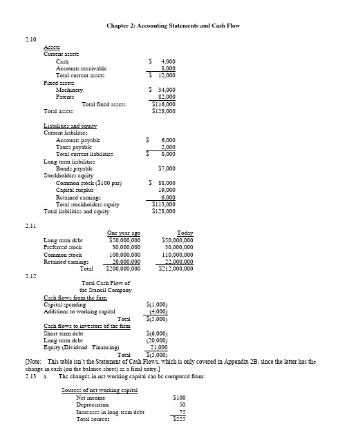
Chapter 2: Accounting Statements and Cash Flow2.10AssetsCurrent assetsCash $ 4,000Accounts receivable 8,000Total current assets $ 12,000Fixed assetsMachinery $ 34,000Patents 82,000Total fixed assets $116,000Total assets $128,000Liabilities and equityCurrent liabilitiesAccounts payable $ 6,000Taxes payable 2,000Total current liabilities $ 8,000Long-term liabilitiesBonds payable $7,000Stockholders equityCommon stock ($100 par) $ 88,000Capital surplus 19,000Retained earnings 6,000Total stockholders equity $113,000Total liabilities and equity $128,0002.11One year ago TodayLong-term debt $50,000,000 $50,000,000Preferred stock 30,000,000 30,000,000Common stock 100,000,000 110,000,000Retained earnings 20,000,000 22,000,000Total $200,000,000 $212,000,0002.12Total Cash Flow ofthe Stancil CompanyCash flows from the firmCapital spending $(1,000)Additions to working capital (4,000)Total $(5,000)Cash flows to investors of the firmShort-term debt $(6,000)Long-term debt (20,000)Equity (Dividend - Financing) 21,000Total $(5,000)[Note: This table isn’t the Statement of Cash Flows, which is only covered in Appendix 2B, since the latter has th e change in cash (on the balance sheet) as a final entry.]2.13 a. The changes in net working capital can be computed from:Sources of net working capitalNet income $100Depreciation 50Increases in long-term debt 75Total sources $225Uses of net working capitalDividends $50Increases in fixed assets* 150Total uses $200Additions to net working capital $25*Includes $50 of depreciation.b.Cash flow from the firmOperating cash flow $150Capital spending (150)Additions to net working capital (25)Total $(25)Cash flow to the investorsDebt $(75)Equity 50Total $(25)Chapter 3: Financial Markets and Net Present Value: First Principles of Finance (Advanced)3.14 $120,000 - ($150,000 - $100,000) (1.1) = $65,0003.15 $40,000 + ($50,000 - $20,000) (1.12) = $73,6003.16 a. ($7 million + $3 million) (1.10) = $11.0 millionb.i. They could spend $10 million by borrowing $5 million today.ii. They will have to spend $5.5 million [= $11 million - ($5 million x 1.1)] at t=1.Chapter 4: Net Present Valuea. $1,000 ⨯ 1.0510 = $1,628.89b. $1,000 ⨯ 1.0710 = $1,967.15c. $1,000 ⨯ 1.0520 = $2,653.30d. Interest compounds on the interest already earned. Therefore, the interest earned inSince this bond has no interim coupon payments, its present value is simply the present value of the $1,000 that will be received in 25 years. Note: As will be discussed in the next chapter, the present value of the payments associated with a bond is the price of that bond.PV = $1,000 /1.125 = $92.30PV = $1,500,000 / 1.0827 = $187,780.23a. At a discount rate of zero, the future value and present value are always the same. Remember, FV =PV (1 + r) t. If r = 0, then the formula reduces to FV = PV. Therefore, the values of the options are $10,000 and $20,000, respectively. You should choose the second option.b. Option one: $10,000 / 1.1 = $9,090.91Option two: $20,000 / 1.15 = $12,418.43Choose the second option.c. Option one: $10,000 / 1.2 = $8,333.33Option two: $20,000 / 1.25 = $8,037.55Choose the first option.d. You are indifferent at the rate that equates the PVs of the two alternatives. You know that rate mustfall between 10% and 20% because the option you would choose differs at these rates. Let r be thediscount rate that makes you indifferent between the options.$10,000 / (1 + r) = $20,000 / (1 + r)5(1 + r)4 = $20,000 / $10,000 = 21 + r = 1.18921r = 0.18921 = 18.921%The $1,000 that you place in the account at the end of the first year will earn interest for six years. The $1,000 that you place in the account at the end of the second year will earn interest for five years, etc. Thus, the account will have a balance of$1,000 (1.12)6 + $1,000 (1.12)5 + $1,000 (1.12)4 + $1,000 (1.12)3= $6,714.61PV = $5,000,000 / 1.1210 = $1,609,866.18a. $1.000 (1.08)3 = $1,259.71b. $1,000 [1 + (0.08 / 2)]2 ⨯ 3 = $1,000 (1.04)6 = $1,265.32c. $1,000 [1 + (0.08 / 12)]12 ⨯ 3 = $1,000 (1.00667)36 = $1,270.24d. $1,000 e0.08 ⨯ 3 = $1,271.25e. The future value increases because of the compounding. The account is earning interest on interest. Essentially, the interest is added to the account balance at the e nd of every compounding period. During the next period, the account earns interest on the new balance. When the compounding period shortens, the balance that earns interest is rising faster.The price of the consol bond is the present value of the coupon payments. Apply the perpetuity formula to find the present value. PV = $120 / 0.15 = $800a. $1,000 / 0.1 = $10,000b. $500 / 0.1 = $5,000 is the value one year from now of the perpetual stream. Thus, the value of theperpetuity is $5,000 / 1.1 = $4,545.45.c. $2,420 / 0.1 = $24,200 is the value two years from now of the perpetual stream. Thus, the value of the perpetuity is $24,200 / 1.12 = $20,000.pply the NPV technique. Since the inflows are an annuity you can use the present value of an annuity factor.ANPV = -$6,200 + $1,200 81.0= -$6,200 + $1,200 (5.3349)= $201.88Yes, you should buy the asset.Use an annuity factor to compute the value two years from today of the twenty payments. Remember, the annuity formula gives you the value of the stream one year before the first payment. Hence, the annuity factor will give you the value at the end of year two of the stream of payments.A= $2,000 (9.8181)Value at the end of year two = $2,000 20.008= $19,636.20The present value is simply that amount discounted back two years.PV = $19,636.20 / 1.082 = $16,834.88The easiest way to do this problem is to use the annuity factor. The annuity factor must be equal to $12,800 / $2,000 = 6.4; remember PV =C A T r. The annuity factors are in the appendix to the text. To use the factor table to solve this problem, scan across the row labeled 10 years until you find 6.4. It is close to the factor for 9%, 6.4177. Thus, the rate you will receive on this note is slightly more than 9%.You can find a more precise answer by interpolating between nine and ten percent.[ 10% ⎤[6.1446 ⎤a ⎡r ⎥bc ⎡6.4 ⎪ d⎣9%⎦⎣6.4177 ⎦By interpolating, you are presuming that the ratio of a to b is equal to the ratio of c to d.(9 - r ) / (9 - 10) = (6.4177 - 6.4 ) / (6.4177 - 6.1446)r = 9.0648%The exact value could be obtained by solving the annuity formula for the interest rate. Sophisticated calculators can compute the rate directly as 9.0626%.[Note: A standard financial calculator’s TVM keys can solve for this rate. With annuity flows, the IRR key on “advanced” financial c alculators is unnecessary.]a. The annuity amount can be computed by first calculating the PV of the $25,000 which youThat amount is $17,824.65 [= $25,000 / 1.075]. Next compute the annuity which has the same present value.A$17,824.65 = C 507.0$17,824.65 = C (4.1002)C = $4,347.26Thus, putting $4,347.26 into the 7% account each year will provide $25,000 five years from today.b. The lump sum payment must be the present value of the $25,000, i.e., $25,000 / 1.075 =$17,824.65The formula for future value of any annuity can be used to solve the problem (see footnote 11 of the text).Option one: This cash flow is an annuity due. To value it, you must use the after-tax amounts. Theafter-tax payment is $160,000 (1 - 0.28) = $115,200. Value all except the first payment using the standard annuity formula, then add back the first payment of $115,200 to obtain the value of this option.AValue = $115,200 + $115,200 30.010= $115,200 + $115,200 (9.4269)= $1,201,178.88Option two: This option is valued similarly. You are able to have $446,000 now; this is already on an after-tax basis. You will receive an annuity of $101,055 for each of the next thirty years. Those payments are taxable when you receive them, so your after-tax payment is $72,759.60 [= $101,055 (1 - 0.28)].AValue = $446,000 + $72,759.60 30.010= $446,000 + $72,759.60 (9.4269)= $1,131,897.47Since option one has a higher PV, you should choose it.et r be the rate of interest you must earn.$10,000(1 + r)12 = $80,000(1 + r)12= 8r = 0.18921 = 18.921%First compute the present value of all the payments you must make for your children’s educati on. The value as of one year before matriculation of one child’s education isA= $21,000 (2.8550) = $59,955.$21,000 415.0This is the value of the elder child’s education fourteen years from now. It is the value of the younger child’s education sixteen years from today. The present value of these isPV = $59,955 / 1.1514 + $59,955 / 1.1516= $14,880.44You want to make fifteen equal payments into an account that yields 15% so that the present value of the equal payments is $14,880.44.A= $14,880.44 / 5.8474 = $2,544.80Payment = $14,880.44 / 15.015This problem applies the growing annuity formula. The first payment is$50,000(1.04)2(0.02) = $1,081.60.PV = $1,081.60 [1 / (0.08 - 0.04) - {1 / (0.08 - 0.04)}{1.04 / 1.08}40]= $21,064.28This is the present value of the payments, so the value forty years from today is$21,064.28 (1.0840) = $457,611.46se the discount factors to discount the individual cash flows. Then compute the NPV of the project. NoticeYou can still use the factor tables to compute their PV. Essentially, they form cash flows that are a six year annuity less a two year annuity. Thus, the appropriate annuity factor to use with them is 2.6198 (= 4.3553 - 1.7355).Year Cash Flow Factor PV0.9091 $636.371$70020.8264 743.769003 1,000 ⎤4 1,000 ⎥ 2.6198 2,619.805 1,000 ⎥6 1,000 ⎦7 1,250 0.5132 641.508 1,375 0.4665 641.44Total $5,282.87NPV = -$5,000 + $5,282.87= $282.87Purchase the machine.Chapter 5: How to Value Bonds and StocksThe amount of the semi-annual interest payment is $40 (=$1,000 ⨯ 0.08 / 2). There are a total of 40 periods;i.e., two half years in each of the twenty years in the term to maturity. The annuity factor tables can be usedto price these bonds. The appropriate discount rate to use is the semi-annual rate. That rate is simply the annual rate divided by two. Thus, for part b the rate to be used is 5% and for part c is it 3%.A+F/(1+r)40PV=C Tra. $40 (19.7928) + $1,000 / 1.0440 = $1,000Notice that whenever the coupon rate and the market rate are the same, the bond is priced at par.b. $40 (17.1591) + $1,000 / 1.0540 = $828.41Notice that whenever the coupon rate is below the market rate, the bond is priced below par.c. $40 (23.1148) + $1,000 / 1.0340 = $1,231.15Notice that whenever the coupon rate is above the market rate, the bond is priced above par.a. The semi-annual interest rate is $60 / $1,000 = 0.06. Thus, the effective annual rate is 1.062 - 1 =0.1236 = 12.36%.A+ $1,000 / 1.0612b. Price = $30 12.006= $748.48A+ $1,000 / 1.0412c. Price = $30 1204.0= $906.15Note: In parts b and c we are implicitly assuming that the yield curve is flat. That is, the yield in year 5applies for year 6 as well.rice = $2 (0.72) / 1.15 + $4 (0.72) / 1.152 + $50 / 1.153= $36.31The number of shares you own = $100,000 / $36.31 = 2,754 sharesPrice = $1.15 (1.18) / 1.12 + $1.15 (1.182) / 1.122 + $1.152 (1.182) / 1.123+ {$1.152 (1.182)(1.06) / (0.12 - 0.06)} / 1.123= $26.95[Insert before last sentence of question: Assume that dividends are a fixed proportion of earnings.] Dividend one year from now = $5 (1 - 0.10) = $4.50Price = $5 + $4.50 / {0.14 - (-0.10)}= $23.75Since the current $5 dividend has not yet been paid, it is still included in the stock price.Chapter 6: Some Alternative Investment Rulesa. Payback period of Project A = 1 + ($7,500 - $4,000) / $3,500 = 2 yearsPayback period of Project B = 2 + ($5,000 - $2,500 -$1,200) / $3,000 = 2.43 yearsProject A should be chosen.b. NPV A = -$7,500 + $4,000 / 1.15 + $3,500 / 1.152 + $1,500 / 1.153 = -$388.96NPV B = -$5,000 + $2,500 / 1.15 + $1,200 / 1.152 + $3,000 / 1.153 = $53.83Project B should be chosen.a. Average Investment:($16,000 + $12,000 + $8,000 + $4,000 + 0) / 5 = $8,000Average accounting return:$4,500 / $8,000 = 0.5625 = 56.25%b. 1. AAR does not consider the timing of the cash flows, hence it does not consider the timevalue of money.2. AAR uses an arbitrary firm standard as the decision rule.3. AAR uses accounting data rather than net cash flows.aAverage Investment = (8000 + 4000 + 1500 + 0)/4 = 3375.00Average Net Income = 2000(1-0.75) = 1500=> AAR = 1500/3375=44.44%a. Solve x by trial and error:-$8,000 + $4,000 / (1 + x) + $3000 / (1 + x)2 + $2,000 / (1 + x)3 = 0x = 6.93%b. No, since the IRR (6.93%) is less than the discount rate of 8%.Alternatively, the NPV @ a discount rate of 0.08 = -$136.62.a. Solve r in the equation:$5,000 - $2,500 / (1 + r) - $2,000 / (1 + r)2 - $1,000 / (1 + r)3- $1,000 / (1 + r)4 = 0By trial and error,IRR = r = 13.99%b. Since this problem is the case of financing, accept the project if the IRR is less than the required rate of return.IRR = 13.99% > 10%Reject the offer.c. IRR = 13.99% < 20%Accept the offer.d. When r = 10%:NPV = $5,000 - $2,500 / 1.1 - $2,000 / 1.12 - $1,000 / 1.13 - $1,000 / 1.14When r = 20%:NPV = $5,000 - $2,500 / 1.2 - $2,000 / 1.22 - $1,000 / 1.23 - $1,000 / 1.24= $466.82Yes, they are consistent with the choices of the IRR rule since the signs of the cash flows change only once.A/ $160,000 = 1.04PI = $40,000 715.0Since the PI exceeds one accept the project.Chapter 7: Net Present Value and Capital BudgetingSince there is uncertainty surrounding the bonus payments, which McRae might receive, you must use the expected value of McRae’s bonuses in the computation of the PV of his contract. McRae’s salary plus the expected value of his bonuses in years one through three is$250,000 + 0.6 ⨯ $75,000 + 0.4 ⨯ $0 = $295,000.Thus the total PV of his three-year contract isPV = $400,000 + $295,000 [(1 - 1 / 1.12363) / 0.1236]+ {$125,000 / 1.12363} [(1 - 1 / 1.123610 / 0.1236]= $1,594,825.68EPS = $800,000 / 200,000 = $4NPVGO = (-$400,000 + $1,000,000) / 200,000 = $3Price = EPS / r + NPVGO= $4 / 0.12 + $3=$36.33Year 0 Year 1 Year 2 Year 3 Year 4 Year 51. Annual Salary$120,000 $120,000 $120,000 $120,000 $120,000 Savings2. Depreciation 100,000 160,000 96,000 57,600 57,6003. Taxable Income 20,000 -40,000 24,000 62,400 62,4004. Taxes 6,800 -13,600 8,160 21,216 21,2165. Operating Cash Flow113,200 133,600 111,840 98,784 98,784 (line 1-4)$100,000 -100,0006. ∆ Net workingcapital7. Investment $500,000 75,792*8. Total Cash Flow -$400,000 $113,200 $133,600 $111,840 $98,784 $74,576*75,792 = $100,000 - 0.34 ($100,000 - $28,800)NPV = -$400,000+ $113,200 / 1.12 + $133,600 / 1.122 + $111,840 / 1.123+ $98,784 / 1.124 + $74,576 / 1.125= -$7,722.52Real interest rate = (1.15 / 1.04) - 1 = 10.58%NPV A = -$40,000+ $20,000 / 1.1058 + $15,000 / 1.10582 + $15,000 / 1.10583= $1,446.76NPV B = -$50,000+ $10,000 / 1.15 + $20,000 / 1.152 + $40,000 / 1.153= $119.17Choose project A.PV = $120,000 / {0.11 - (-0.06)}t = 0 t = 1 t = 2 t = 3 t = 4 t = 5 t = 6 ...$12,000 $6,000 $6,000 $6,000$4,000$12,000 $6,000 $6,000 ...The present value of one cycle is:A+ $4,000 / 1.064PV = $12,000 + $6,000 306.0= $12,000 + $6,000 (2.6730) + $4,000 / 1.064= $31,206.37The cycle is four years long, so use a four year annuity factor to compute the equivalent annual cost (EAC).AEAC = $31,206.37 / 406.0= $31,206.37 / 3.4651= $9,006The present value of such a stream in perpetuity is$9,006 / 0.06 = $150,100o evaluate the word processors, compute their equivalent annual costs (EAC).BangAPV(costs) = (10 ⨯ $8,000) + (10 ⨯ $2,000) 414.0= $80,000 + $20,000 (2.9137)= $138,274EAC = $138,274 / 2.9137= $47,456IOUAPV(costs) = (11 ⨯ $5,000) + (11 ⨯ $2,500) 3.014- (11 ⨯ $500) / 1.143= $55,000 + $27,500 (2.3216) - $5,500 / 1.143= $115,132EAC = $115,132 / 2.3216= $49,592BYO should purchase the Bang word processors.Chapter 8: Strategy and Analysis in Using Net Present ValueThe accounting break-even= (120,000 + 20,000) / (1,500 - 1,100)= 350 units. The accounting break-even= 340,000 / (2.00 - 0.72)= 265,625 abalonesb. [($2.00 ⨯ 300,000) - (340,000 + 0.72 ⨯ 300,000)] (0.65)= $28,600This is the after tax profit.Chapter 9: Capital Market Theory: An Overviewa. Capital gains = $38 - $37 = $1 per shareb. Total dollar returns = Dividends + Capital Gains = $1,000 + ($1*500) = $1,500 On a per share basis, this calculation is $2 + $1 = $3 per sharec. On a per share basis, $3/$37 = 0.0811 = 8.11% On a total dollar basis, $1,500/(500*$37) = 0.0811 = 8.11%d. No, you do not need to sell the shares to include the capital gains in the computation of the returns. The capital gain is included whether or not you realize the gain. Since you could realize the gain if you choose, you should include it.The expected holding period return is:()[]%865.1515865.052$/52$75.54$50.5$==-+There appears to be a lack of clarity about the meaning of holding period returns. The method used in the answer to this question is the one used in Section 9.1. However, the correspondence is not exact, because in this question, unlike Section 9.1, there are cash flows within the holding period. The answer above ignores the dividend paid in the first year. Although the answer above technically conforms to the eqn at the bottom of Fig. 9.2, the presence of intermediate cash flows that aren’t accounted for renders th is measure questionable, at best. There is no similar example in the body of the text, and I have never seen holding period returns calculated in this way before.Although not discussed in this book, there are two generally accepted methods of computing holding period returns in the presence of intermediate cash flows. First, the time weighted return calculates averages (geometric or arithmetic) of returns between cash flows. Unfortunately, that method can’t be used here, because we are not given the va lue of the stock at the end of year one. Second, the dollar weighted measure calculates the internal rate of return over the entire holding period. Theoretically, that method can be applied here, as follows: 0 = -52 + 5.50/(1+r) + 60.25/(1+r)2 => r = 0.1306.This produces a two year holding period return of (1.1306)2 – 1 = 0.2782. Unfortunately, this book does not teach the dollar weighted method.In order to salvage this question in a financially meaningful way, you would need the value of the stock at the end of one year. Then an illustration of the correct use of the time-weighted return would be appropriate. A complicating factor is that, while Section 9.2 illustrates the holding period return using the geometric return for historical data, the arithmetic return is more appropriate for expected future returns.E(R) = T-Bill rate + Average Excess Return = 6.2% + (13.0% -3.8%) = 15.4%. Common Treasury Realized Stocks Bills Risk Premium -7 32.4% 11.2% 21.2%-6 -4.9 14.7 -19.6-5 21.4 10.5 10.9 -4 22.5 8.8 13.7 -3 6.3 9.9 -3.6 -2 32.2 7.7 24.5 Last 18.5 6.2 12.3 b. The average risk premium is 8.49%.49.873.125.246.37.139.106.192.21=++-++- c. Yes, it is possible for the observed risk premium to be negative. This can happen in any single year. The.b.Standard deviation = 03311.0001096.0=.b.Standard deviation = = 0.03137 = 3.137%.b.Chapter 10: Return and Risk: The Capital-Asset-Pricing Model (CAPM)a. = 0.1 (– 4.5%) + 0.2 (4.4%) + 0.5 (12.0%) + 0.2 (20.7%) = 10.57%b.σ2 = 0.1 (–0.045 – 0.1057)2 + 0.2 (0.044 – 0.1057)2 + 0.5 (0.12 – 0.1057)2+ 0.2 (0.207 – 0.1057)2 = 0.0052σ = (0.0052)1/2 = 0.072 = 7.20%Holdings of Atlas stock = 120 ⨯ $50 = $6,000 ⨯ $20 = $3,000Weight of Atlas stock = $6,000 / $9,000 = 2 / 3Weight of Babcock stock = $3,000 / $9,000 = 1 / 3a. = 0.3 (0.12) + 0.7 (0.18) = 0.162 = 16.2%σP 2= 0.32 (0.09)2 + 0.72 (0.25)2 + 2 (0.3) (0.7) (0.09) (0.25) (0.2)= 0.033244σP= (0.033244)1/2 = 0.1823 = 18.23%a.State Return on A Return on B Probability1 15% 35% 0.4 ⨯ 0.5 = 0.22 15% -5% 0.4 ⨯ 0.5 = 0.23 10% 35% 0.6 ⨯ 0.5 = 0.34 10% -5% 0.6 ⨯ 0.5 = 0.3b. = 0.2 [0.5 (0.15) + 0.5 (0.35)] + 0.2[0.5 (0.15) + 0.5 (-0.05)]+ 0.3 [0.5 (0.10) + 0.5 (0.35)] + 0.3 [0.5 (0.10) + 0.5 (-0.05)]= 0.135= 13.5%Note: The solution to this problem requires calculus.Specifically, the solution is found by minimizing a function subject to a constraint. Calculus ability is not necessary to understand the principles behind a minimum variance portfolio.Min { X A2 σA2 + X B2σB2+ 2 X A X B Cov(R A , R B)}subject to X A + X B = 1Let X A = 1 - X B. Then,Min {(1 - X B)2σA2 + X B2σB2+ 2(1 - X B) X B Cov (R A, R B)}Take a derivative with respect to X B.d{∙} / dX B = (2 X B - 2) σA2+ 2 X B σB2 + 2 Cov(R A, R B) - 4 X B Cov(R A, R B)Set the derivative equal to zero, cancel the common 2 and solve for X B.X BσA2- σA2+ X B σB2 + Cov(R A, R B) - 2 X B Cov(R A, R B) = 0X B = {σA2 - Cov(R A, R B)} / {σA2+ σB2 - 2 Cov(R A, R B)}andX A = {σB2 - Cov(R A, R B)} / {σA2+ σB2 - 2 Cov(R A, R B)}Using the data from the problem yields,X A = 0.8125 andX B = 0.1875.a. Using the weights calculated above, the expected return on the minimum variance portfolio isE(R P) = 0.8125 E(R A) + 0.1875 E(R B)= 0.8125 (5%) + 0.1875 (10%)= 5.9375%b. Using the formula derived above, the weights areX A = 2 / 3 andX B = 1 / 3c. The variance of this portfolio is zero.σP 2= X A2 σA2 + X B2σB2+ 2 X A X B Cov(R A , R B)= (4 / 9) (0.01) + (1 / 9) (0.04) + 2 (2 / 3) (1 / 3) (-0.02)= 0This demonstrates that assets can be combined to form a risk-free portfolio.14.2%= 3.7%+β(7.5%) ⇒β = 1.40.25 = R f + 1.4 [R M– R f] (I)0.14 = R f + 0.7 [R M– R f] (II)(I) – (II)=0.11 = 0.7 [R M– R f] (III)[R M– R f ]= 0.1571Put (III) into (I) 0.25 = R f + 1.4[0.1571]R f = 3%[R M– R f ]= 0.1571R M = 0.1571 + 0.03= 18.71%a. = 4.9% + βi (9.4%)βD= Cov(R D, R M) / σM 2 = 0.0635 / 0.04326 = 1.468= 4.9 + 1.468 (9.4) = 18.70%Weights:X A = 5 / 30 = 0.1667X B = 10 / 30 = 0.3333X C = 8 / 30 = 0.2667X D = 1 - X A - X B - X C = 0.2333Beta of portfolio= 0.1667 (0.75) + 0.3333 (1.10) + 0.2667 (1.36) + 0.2333 (1.88)= 1.293= 4 + 1.293 (15 - 4) = 18.22%a. (i) βA= ρA,MσA / σMρA,M= βA σM / σA= (0.9) (0.10) / 0.12= 0.75(ii) σB= βB σM / ρB,M= (1.10) (0.10) / 0.40= 0.275(iii) βC= ρC,MσC / σM= (0.75) (0.24) / 0.10= 1.80(iv) ρM,M= 1(v) βM= 1(vi) σf= 0(vii) ρf,M= 0(viii) βf= 0b. SML:E(R i) = R f + βi {E(R M) - R f}= 0.05 + (0.10) βiSecurity βi E(R i)A 0.13 0.90 0.14B 0.16 1.10 0.16C 0.25 1.80 0.23Security A performed worse than the market, while security C performed better than the market.Security B is fairly priced.c. According to the SML, security A is overpriced while security C is under-priced. Thus, you could invest in security C while sell security A (if you currently hold it).a. The typical risk-averse investor seeks high returns and low risks. To assess thetwo stocks, find theReturns:State of economy ProbabilityReturn on A*Recession 0.1 -0.20 Normal 0.8 0.10 Expansion0.10.20* Since security A pays no dividend, the return on A is simply (P 1 / P 0) - 1. = 0.1 (-0.20) + 0.8 (0.10) + 0.1 (0.20) = 0.08 = 0.09 This was given in the problem.Risk:R A - (R A -)2 P ⨯ (R A -)2 -0.28 0.0784 0.00784 0.02 0.0004 0.00032 0.12 0.0144 0.00144 Variance 0.00960Standard deviation (R A ) = 0.0980βA = {Corr(R A , R M ) σ(R A )} / σ(R M ) = 0.8 (0.0980) / 0.10= 0.784βB = {Corr(R B , R M ) σ(R B )} / σ(R M ) = 0.2 (0.12) / 0.10= 0.24The return on stock B is higher than the return on stock A. The risk of stock B, as measured by itsbeta, is lower than the risk of A. Thus, a typical risk-averse investor will prefer stock B.b. = (0.7) + (0.3) = (0.7) (0.8) + (0.3) (0.09) = 0.083σP 2= 0.72 σA 2 + 0.32 σB 2 + 2 (0.7) (0.3) Corr (R A , R B ) σA σB = (0.49) (0.0096) + (0.09) (0.0144) + (0.42) (0.6) (0.0980) (0.12) = 0.0089635 σP = = 0.0947 c. The beta of a portfolio is the weighted average of the betas of the components of the portfolio. βP = (0.7) βA + (0.3) βB = (0.7) (0.784) + (0.3) (0.240) = 0.621Chapter 11:An Alternative View of Risk and Return: The Arbitrage Pricing Theorya. Stock A:()()R R R R R A A A m m Am A=+-+=+-+βεε105%12142%...Stock B:()()R R R R R B B m m Bm B=+-+=+-+βεε130%098142%...Stock C:()R R R R R C C C m m Cm C=+-+=+-+βεε157%137142%)..(.b.()[]()[]()[]()()()()()()[]()()CB A m cB A m c m B m A m CB A P 25.045.030.0%2.14R 1435.1%925.1225.045.030.0%2.14R 37.125.098.045.02.130.0%7.1525.0%1345.0%5.1030.0%2.14R 37.1%7.1525.0%2.14R 98.0%0.1345.0%2.14R 2.1%5.1030.0R 25.0R 45.0R 30.0R ε+ε+ε+-+=ε+ε+ε+-+++++=ε+-++ε+-++ε+-+=++= c.i.()R R R A B C =+-==+-==+-=105%1215%142%)1113%09815%142%)137%157%13715%142%168%..(..46%.(......ii.R P =+-=12925%1143515%142%)138398%..(..To determine which investment investor would prefer, you must compute the variance of portfolios created bymany stocks from either market. Note, because you know that diversification is good, it is reasonable to assume that once an investor chose the market in which he or she will invest, he or she will buy many stocks in that market.Known:E EF ====001002 and and for all i.i σσεε..Assume: The weight of each stock is 1/N; that is, X N i =1/for all i.If a portfolio is composed of N stocks each forming 1/N proportion of the portfolio, the return on the portfolio is 1/N times the sum of the returns on the N stocks. Recall that the return on each stock is 0.1+βF+ε.()()()()()()[]()()()()()()()[]()[]()[]()()[]()()()()()j i 2j i 22j i i 2222222222P P P P iP ,0.04Corr 0.01,Cov s =isvariance the ,N as limit In the ,Cov 1/N 1s 1/N s )(1/N 1/N F 2F E 1/N F E 0.10.1/N F 0.1E R E R E R Var 0.101/N 00.1E 1/N F E 0.11/N F 0.1E R E 1/N F 0.1F 0.1(1/N)R 1/N R εε+β=εε+β∞⇒εε-+ε+β=ε∑+εβ+β=ε+β=-ε+β+=-==+β+=ε+β+=ε∑+β+=ε+β+=ε+β+==∑∑∑∑∑∑∑∑()()()()()()Thus,F R f E R E R Var R Corr Var R Corr ii ip P p i j PijR 1i =++=++===+=+010*********002250040002500412212111222.........,,εεεεεεa.()()()()Corr Corr Var R Var R i j i j p pεεεε112212000225000225,,..====Since Var ()()R p 1 Var R 2p 〉, a risk averse investor will prefer to invest in the second market.b. Corr ()()εεεε112090i j j ,.,== and Corr 2i()()Var R Var R pp120058500025==..。

European Financial Management,V ol.15,No.1,2009,47–65doi:10.1111/j.1468-036X.2007.00420.xCash Flow Sensitivity of InvestmentArmen HovakimianZicklin School of Business,Baruch College,One Bernard Baruch Way,Box B10–225,New York, NY10010,USAE-mail:armen hovakimian@Gayan´e HovakimianFordham University,Graduate School of Business,113West60th Street,New York,NY10023, USAE-mail:hovakimian@AbstractInvestment cash flow sensitivity is associated with both underinvestment when cash flows are low and overinvestment when cash flows are high.The accessibility of external capital is positively correlated with cash flows,intensifying investment cash flow sensitivity.Managers actively counteract the variations in internal and external liquidity by accumulating working capital when liquidity is high and draining it when liquidity is low.These results imply that cash flow sensitive firms face financial constraints,which are binding in low cash flow years.Traditional indicators of financial constraints,such as size and dividend payout,successfully distinguish firms that may potentially face constraints,but are less successful in distinguishing between periods of tight and relaxed constraints.These periods are much more clearly separated by the KZ index,which,on the other hand,is less successful in identifying firms that are likely to face liquidity constraints.Keywords:investment cash flow sensitivity,financial constraints,investment,man-agerial overconfidenceJEL classification:G30,G31,G321.IntroductionThe sensitivity of investment expenditures to internal cash flows is a well-documented phenomenon in the financial economics literature.In a seminal study,Fazzari et al., (1988)show that,after controlling for growth opportunities,corporate investment is sensitive to cash flow and more so for firms with low dividend payout.The authors conclude that the strong positive effect of internal funds on investment is caused by theWe would like to thank an anonymous referee,John Doukas(Managing Editor),the participants of European Financial Management Association(2005)and Financial Manage-ment Association(2006)annual meetings,as well as the seminar participants at Fordham University and Baruch College for helpful comments.C 2007The AuthorsJournal compilation C 2007Blackwell Publishing Ltd.48Armen Hovakimian and Gayan´e Hovakimianliquidity constraints faced by firms with significant differences between the costs of external and internal capital.A large body of follow-up literature finds support for this argument.1Some other studies,however,show that investment cash flow sensitivity may be observed even in frictionless markets for reasons other than financial constraints. Specifically,because of difficulty of measuring marginal investment opportunities (Tobin’s Q),cash flow may convey information about investment opportunities that is not reflected in the estimated Q.In such cases,the observed cross-sectional variations in investment-cash flow sensitivity may simply be due to variations in Q measurement error.2Alternatively,cross-sectional differences in investment cash flow sensitivity may be observed if cash flow is a better proxy for growth opportunities for certain types of firms.3Y et another alternative explanation is that cash flow sensitivity of investment reflects the managers’tendency to overinvest when they have access to internal funds.4 Our empirical approach is different from those applied in previous studies.Most of the previous studies draw conclusions based on differences in cash flow sensitivities estimated for sub-samples formed using ex ante proxies for financial constraints,such as dividend payout and size.5However,such conclusions critically depend on the definition of and the choice of the proxy for financial constraints.For example,using alternative classification approaches,Kaplan and Zingales(1997)and Cleary(1999)find higher levels of cash flow sensitivity for firms that are least likely to be financially constrained. Unlike these studies,we make no assumptions about what causes investment cash flow sensitivity.We examine whether investment cash flow sensitivity is associated with economically significant distortions in the level and timing of investment expenditures in two steps.First,we empirically identify firms with relatively high and low investment cash flow sensitivity.Next,we explore the differences in the dynamics of their investment and methods of financing across periods of high and low cash flows.This analysis,in 1Higher investment-cash flow sensitivity is also observed for firms that are young or small (Devereux and Schiantarelli,1990;Oliner and Rudebusch,1992;Kadapakkam et al.,1998; Shin and Kim,2002)have low or no credit rating(Calomiris et al.,1996),for independent firms,as opposed to firms affiliated with industrial groups(Hoshi et al.,1991;Shin and Park,1999).For a more complete survey,see Hubbard(1998)and Schiantarelli(1996).2For example,Erickson and Whited(2000)argue that the significance of cash flow disappears when they use measurement-error-consistent GMM estimators.Cummins et al. (1999)control for expected future profits and find insignificant cash flow coefficients. Gilchrist and Himmelberg(1995)find that,at least in some cases,the significance of cash flow is due to its association with investment opportunities.3Alti(2003)presents a model where the link between investment and cash flow is stronger for high growth firms because managers adjust current investment in response to cash flow realisations,which reflect current growth opportunities.4Jensen(1986)argues that managers would rather invest in negative NPV projects than pay out the free cash flow to investors.Pawlina and Renneboog(2005)find support for this hypothesis and report that investment-cash flow sensitivity is primarily driven by overinvestment by managers with high discretion.Morgado and Pindado(2003)examine the relation between investment and firm value and find evidence of both under-and overinvestment in the data.5Among the few exceptions,Hovakimian and Titman(2006)use a switching regression framework to simultaneously estimate the two regimes of the investment regression along with the factors that determine these regimes.C 2007The AuthorsJournal compilation C 2007Blackwell Publishing LtdCash Flow Sensitivity of Investment49 turn,provides basis for drawing inferences about factors underlying investment cash flow sensitivity.We find that investment cash flow sensitivity is associated with underinvestment when cash flows are low and overinvestment when cash flows are high.Our conclusions are based on two key pieces of evidence.First,we find that,in low cash flow years,cash flow sensitive firms invest less,while in high cash flow years they invest more than otherwise comparable firms.Second,our results imply that,in low cash flow years, managers would like to invest more than the financing sources permit.They act as if marginal investment opportunities are not as low as implied by low market-to-book ratios and cash flows.The shortfall of funds for capital expenditures is covered with funds released by draining financial slack and net working capital to abnormally low levels.In contrast,in high cash flow years,managers invest less than the financing sources permit.Instead,they accumulate excess slack and net working capital,acting as if they anticipate future shortage of funds.These patterns of investment,along with patterns of internal and external financing, imply that cash flow sensitive firms face financial constraints,but that the severity of these constraints varies across the cash flow cycle.The constraints are binding in low cash flow years when the shortage of internally generated funds is exacerbated by lower availability of external capital.Debt is less available because cash flow sensitive firms are significantly overlevered in low cash flow years,implying that the borrowing costs are likely to be high.6External equity is also likely to be viewed as expensive since the market-to-book ratios of cash flow sensitive firms are low in these years.While the literature on corporate investment traditionally treats market-to-book ratios as the market’s assessment of firms’growth opportunities,recent studies of corporate financing decisions increasingly argue that equity-financing decisions are affected by managerial perceptions of mispricing and use market-to-book as a proxy for such mispricing.7In contrast,high cash flow levels mark periods of increased availability of not only internal capital but also external capital due to relatively low leverage and high equity valuations.As a result,the significant levels of internally generated funds are supplemented by large quantities of new debt and equity financing,implying that financing constraints are not binding in high cash flow years.While our conclusion that cash flow sensitive firms face financial constraints is consistent with Fazzari et al.(1988)and the supporting literature,the finding that these constraints are not always binding is new.We,next,examine how traditional proxies for financial constraints,such as firm size,dividend payout and investment grade rating, vary across cash flow sensitive and cash flow insensitive firms and across their cash flow cycle.Of particular interest is their comparison with the KZ-index that,when applied as a proxy for financial constraints,does not support the link between financial constraints and investment cash flow sensitivity.8We find that size,dividend payout,and investment grade rating do identify firms that are likely to face financial constraints,but do not vary significantly across years of 6Hovakimian et al.(2001)find that firms are reluctant to issue debt when their debt ratios are relatively high,since excessive leverage increases the probability of financial distress. 7Baker and Wurgler(2002)argue that firms are reluctant to issue equity when their market-to-book ratios are relatively low because managers perceive their shares as undervalued.8KZ-index is an index based on the estimation of the determinants of the constrained vs. unconstrained financial status from Kaplan and Zingales(1997).The index is discussed in detail later in the paper.C 2007The AuthorsJournal compilation C 2007Blackwell Publishing Ltd50Armen Hovakimian and Gayan´e Hovakimianbinding and non-binding liquidity constraints.In contrast,KZ index distinguishes between years with binding and non-binding constraints,but is less helpful in identifying firms that are likely to face financial constraints.Thus,the traditional proxies for finan-cial constraints and the KZ index reflect two distinct aspects of financial constraints. Our results help explain why many studies(e.g.,Almeida et al.2004)find that,unlike other indicators of financial constraints,higher levels of KZ index are associated with lower cash flow sensitivity of cash.Specifically,we find that fixed effects regression estimates of cash flow sensitivity are the highest in high cash flow periods of cash flow sensitive firms.Y et,based on KZ index,these are the least constrained firm-years in our sample.These results are not surprising in the light of our finding that financial constraints are not binding in high cash flow periods allowing CF-sensitive firms to overinvest.We also find that fixed effects regression estimates of cash flow sensitivity are the lowest in low cash flows periods of cash flow sensitive firms,which KZ index identifies as the most constrained firm-years in our sample.Our results indicate that this effect arises because when cash flows are too low,the variation in their level has no significant effect on capital investment.The paper proceeds as follows.Section2describes the sample and separates cash flow sensitive and cash flow insensitive firms.Section3examines the dynamics of investment and financing behavior of cash flow sensitive and cash flow insensitive firms. Section4examines the traditional proxies of financial constraints and the KZ index for cash flow sensitive and insensitive firms and across the firms’cash flow cycle. Section5summarises our conclusions.2.The Sample DescriptionOur sample is drawn from COMPUSTAT and covers the1985–2003time period.9 We exclude financial institutions(SIC codes6000–6999)and firms with book values of assets,net fixed capital,or sales less than one million dollars.To minimise the influence of outliers in our analysis,we replace extreme observations of all ratio variables with missing values.10Since our analysis uses variables formed on the basis of time series of firm-level observations,only firms with at least two years in the time series are kept in the sample.11 The sample does not have other survival requirements and includes a substantial number of firms that no longer exist.The final sample is an unbalanced panel dataset of60,285 observations representing7,176firms.2.1.Separating cash flow sensitive and cash flow insensitive firmsOur goal in this section is to split the sample into subsamples of firms with relatively high and relatively low cash flow sensitivity of investment.12We identify cash flow 9Compustat starts reporting Standard and Poors’credit ratings in1985.10Extreme observations include values in the99th percentile and,for variables with negative values,also those in the first percentile.11We have performed an analysis of the sensitivity of our results to the exclusion of firms with less than five and,alternatively,less than ten observations in the time series.Our results remained qualitatively the same.12Investment is defined as capital expenditures(Compustat Item128)divided by the beginning-of-period net capital(Item8).C 2007The AuthorsJournal compilation C 2007Blackwell Publishing LtdCash Flow Sensitivity of Investment51 sensitive firms in two steps.First,for each firm in our sample,we gauge the firm level investment cash flow sensitivity(CFSI)by calculating the difference between the cash flow weighted time-series average investment of a firm and its simple arithmetic time-series average investment.13This value is higher for firms that tend to invest more in years with relatively high cash flows and less in years with low cash flows.To account for the possibility that investment may be financed with cash flows from the previous fiscal year,we also calculate the CFSI based on cash flow that is lagged relative to investment.CFSI attempts to capture the economic significance of the variation in investment associated with variation in cash flow.CFSI will be low,for example,if there is little variation in cash flows,even if the response of investment to a dollar change in cash flow is significant.Similarly,CFSI will be low if the variation in investment induced by variation in cash flow is small relative to the average level of investment.14To see whether our indicator variable correctly classifies firms in the traditional regression framework,we estimate cross-section time-series investment regressions with fixed firm effects for our full sample and for firms with CFSI above0.05(hereafter, CF-sensitive firms)and with CFSI below0.05(hereafter,CF-insensitive firms),based on current or lagged cash flow:Inv it=αi+β1MB it+β2CF it+β3CF it−1+εit(1) Table1shows the results of estimation of two versions of regression model(1).The dependent variable in both regressions is investment.The independent variables in the first regression,presented in Panel A,are the beginning of period market-to-book ratio of assets,MB t,as a proxy for Tobin’s Q,and cash flow,CF t.15The second regression, presented in Panel B,contains previous period’s cash flow,CF t−1,as an additional regressor to account for the possibility that investment may be financed with cash flows from the previous fiscal year.The reported statistics reflect standard errors robust to heteroscedasticity and clustering by year.Both sets of results confirm the evidence of cash flow sensitivity of investment for our full sample.However,the relation between investment and cash flow is significantly positive for firms classified as CF-sensitive(0.101)and insignificant for firms classified as CF-insensitive(−0.001).The differences in CF-sensitivity are significant not only statistically,but also economically.The threshold of0.05used for CFSI is ad hoc.However,our sample separation does not aim to reflect any particular economic phenomenon such as,for example,13CFSI is calculated asnt=1(I it×C F it/nt=1C F it)−1nnt=1I it,where,n is the number ofannual observations for firm i,and t is the time period.CF is the cash flow,as defined earlier.I is the investment,as defined earlier.To avoid negative and extreme weight values, negative cash flows in this formula are set to zero.14CFSI can alternatively be expressed as CFSI=ρσIσC F/C F=[ρσI]×[σC F/C F].The first term in brackets is the portion of investment volatility that is due to its correlation with cash flow.The second bracketed term is the coefficient of variation of cash flow.15Market-to-book is(total assets(Item6)–book value of equity(Item60)–deferred taxes (Item35)+market value of equity(Item199×Item25))/total assets.Cash flow is defined as(income before extraordinary items(Item18)+depreciation and amortisation(Item14)) divided by the beginning-of-period net capital.C 2007The AuthorsJournal compilation C 2007Blackwell Publishing Ltd52Armen Hovakimian and Gayan´e HovakimianTable1Investment regressionsFixed firm effects panel regressions of investment.Investment is capital expenditures scaled by lagged net capital.Market-to-book is(total assets−book value of equity−deferred taxes+market value of equity)/total assets.CF is cash flow,defined as(earnings before extraordinary items+depreciation) over lagged net capital.CF(−1)is lagged cash flow.The reported statistics reflect standard errors adjusted for heteroscedasticity and clustering.Coefficient estimates significantly different from zero at5%and1%level are marked∗and∗∗,respectively.Full sample CF-insensitive CF-sensitiveCoeff.t-stat.Coeff.t-stat.Coeff.t-stat. Panel A:Market-to-book0.084∗∗16.20.043∗∗16.40.110∗∗15.9 CF0.074∗∗12.4−0.001−0.10.101∗∗10.9R-sq.0.4670.6320.440 Observations60,28539,75220,533Panel B:Market-to-book0.072∗∗14.50.043∗∗15.20.090∗∗14.5 CF0.060∗∗12.2−0.001−0.30.087∗∗11.6 CF(−1)0.062∗∗14.50.0040.90.074∗∗15.0 R-sq.0.4840.6320.467 Observations60,28539,75220,533financial constraints.Our goal is simply to split the sample into two subsamples that differ significantly in terms of cash flow sensitivity of investment.The coefficient estimates for cash flow variables in Table1imply that we have clearly achieved this limited goal.That said,we have experimented with threshold values as low as0.02and as high as0.1.16The qualitative patterns reported in the paper have not changed.Table2reports the mean values of investment,cash flow,and other firm character-istics,separately for CF-sensitive and CF-insensitive firms.17Overall,the results are consistent with the findings of earlier studies.Cash flow sensitive firms have higher rates of investment,but lower cash flows,they are smaller,less likely to pay dividends, and have somewhat lower leverage ratios,but higher tangibility,market-to-book,and R&D expenses.These firms also raise more external funds and keep higher levels of slack.3.Investment and Financing Behaviour of CF-Sensitive and CF-Insensitive FirmsIn this section,we examine whether investment-cash flow sensitivity is associated with economically significant distortions in firm investment and financing behaviour and 16The mean and the median values of CFSI in our sample are0.054and0.041,respectively. 17The reported values are the cross-sectional means of the firm-level mean values.C 2007The AuthorsJournal compilation C 2007Blackwell Publishing LtdCash Flow Sensitivity of Investment53Table2Average firm characteristics by cash flow sensitivity typeThe reported means are cross-sectional averages of time-series averages for individual firms.Cash flow is(earnings before extraordinary items+depreciation)over lagged net capital.Investment is capital expenditures scaled by lagged net equity issued is the difference between equity issued and equity repurchased,scaled by net debt issued is the change in the book value of long-term and short-term debt scaled by net capital.Financial slack is cash and marketable securities over net capital.Dividend payout indicator is set to1if a firm pays dividends.Leverage is the sum of short-term and long-term debt divided by total assets.Market-to-book is the(total assets−book value of equity−deferred taxes+market value of equity)/total assets.Variable Full sample CF-insensitive CF-sensitive CF-sensitivity0.054−0.0030.132 Investment0.3040.2440.387 Cash flow0.3060.3280.274 Equity issued0.1560.0910.245 Debt issued0.1730.1420.215 Financial slack0.9590.7571.238 Dividend payout indicator0.2880.4010.130 Leverage0.2720.2810.259 Market-to-book1.5911.5211.688 Sales(in million$)927.41308.0399.8 Observations7,1764,1693,007 why.In order to address these questions,we study firm investment and financing in periods of low and high cash flows.We define a year as low(high)cash flow if the cash flow in that year is lower(higher)than the firm’s time-series average cash flow.The average cash flows are presented in the first row of Table3,which shows that,for cash flow sensitive firms,the difference between average cash flows in high and low cash flow periods is2.5times larger than it is for cash flow insensitive firms.3.1.Investment across the cash flow cycleAverage capital expenditures in low-and high cash flow periods are presented in Table3.The results show that,in low cash flow years,CF-sensitive and insensitive firms have similar investment rates(0.210and0.238,respectively).In high cash flow years,however,the investment rates of CF-sensitive firms(0.507)are almost double those of CF-insensitive firms(0.269).To see whether firms overinvest or underinvest,we calculate three measures of excess investment.The first measure is simply the difference between the capital expenditures of a firm and the average capital expenditures for firms in the same year and industry(based on the two-digit SIC code).In order to control for firm-specific growth opportunities,the second measure is obtained by estimating the following cross-sectional regression of investment on market-to-book ratio,separately,for each year and industry:Inv i=β0+β1MB i+εi(2) C 2007The AuthorsJournal compilation C 2007Blackwell Publishing Ltd54Armen Hovakimian and Gayan´e HovakimianTable3Investment across the cash flow cycle by investment-cash flow sensitivity typeA year is defined as low(high)cash flow if the cash flow is less(greater)than the firm’s time series mean.Cash flow is(earnings before extraordinary items+depreciation)over lagged net capital. Investment is capital expenditures scaled by lagged net investment is the change in net capital over lagged net capital.Asset growth is the change in assets over lagged assets.Sales growth is the change in sales over lagged sales.Excess value(industry,year)is the difference between the value of the firm characteristic and the average value for firms in the same year and industry(based on the two-digit SIC code).Excess value(industry,year,MB)is the residual of a cross-sectional regression of the firm characteristic on market-to-book ratio estimated separately for each year and industry. Spell length is the average length of low and high cash flow periods excluding truncated cases.Values significantly different from zero at5%and1%level are marked∗and∗∗,respectively.High cash flow year values significantly different from low cash flow year values at5%and1%level are marked x and xx,respectively.CF-insensitive CF-sensitive High vs.low cash flow years Low High Low High Cash flow0.165∗∗0.582∗∗xx−0.089∗∗0.944∗∗xx Investment0.210∗∗0.269∗∗xx0.238∗∗0.507∗∗xx Excess investment(industry,year)−0.048∗∗−0.003xx−0.050∗∗0.191∗∗xxExcess investment(industry,year,MB)−0.034∗∗−0.012∗∗xx−0.037∗∗0.160∗∗xx Excess investment(ind.,year,MB,size)−0.031∗∗−0.009∗∗xx−0.040∗∗0.151∗∗xx Net investment0.046∗∗0.156∗∗xx0.0030.330∗∗xx Excess net investment(industry,year)−0.057∗∗0.033∗∗xx−0.097∗∗0.198∗∗xx Excess net investment(industry,year,MB)−0.043∗∗0.024∗∗xx−0.083∗∗0.165∗∗xx Excess net investment(ind.,year,MB,size)−0.040∗∗0.025∗∗xx−0.085∗∗0.157∗∗xx Asset growth0.055∗∗0.179∗∗xx0.007∗0.298∗∗x Excess asset growth(industry,year)−0.055∗∗0.050∗∗xx−0.102∗∗0.160∗∗xx Excess asset growth(industry,year,MB)−0.041∗∗0.039∗∗xx−0.088∗∗0.131∗∗xx Excess asset growth(ind.,year,MB,size)−0.038∗∗0.040∗∗xx−0.089∗∗0.125∗∗xx Sales growth0.055∗∗0.158∗∗xx0.034∗∗0.271∗∗xx Excess sales growth(industry,year)−0.048∗∗0.035∗∗xx−0.073∗∗0.136∗∗xx Excess sales growth(industry,year,MB)−0.038∗∗0.028∗∗xx−0.063∗∗0.114∗∗xx Excess sales growth(ind.,year,MB,size)−0.034∗∗0.031∗∗xx−0.067∗∗0.104∗∗xx Spell length 3.892∗∗ 3.844∗∗xx 3.984∗∗ 3.436∗∗xx Observations20,06019,69212,0428,491The residuals of these regressions are then used to measure excess investment.The third measure of excess investment is similar to the second one,except regression(2) is modified to include size as an additional regressor.18The excess investment of CF-sensitive firms is significantly positive in high cash flow years and significantly negative in low cash flow years based on all three measures. The deviations from‘normal’investment in Table3are economically significant.For18Since CF-sensitive firms tend to be smaller,their investment rates may be higher than the average industry rates.Likewise,the investment rates of CF-insensitive firms may be lower than the average industry rates.C 2007The AuthorsJournal compilation C 2007Blackwell Publishing LtdCash Flow Sensitivity of Investment55 example,the average excess investment of−0.050implies that in low cash flow years,the investment of CF-sensitive firms is more than17%lower than their industry mean.The average excess investment of0.191implies that in high cash flow years,the investment of CF-sensitive firms exceeds their industry mean by more than50%.The excess investment of CF-insensitive firms is negative in both low-and high cash flow years.It is possible that CF-insensitive firms are less capital intensive and, therefore,their low investment rates are not really abnormal.We,therefore,also present excess values of investment defined in terms of net investment(change in net capital). This measure is different from capital expenditures because it is net of depreciation and includes the effects of acquisitions and divestitures.If depreciation is a reasonable approximation of the true rate at which the existing fixed assets of a firm have to be replaced in order to maintain the current levels of production,then investment net of depreciation is a better measure of new investment.The results show that the net investment of CF-sensitive firms is not significantly different from zero in low cash flow years,while it is significantly positive in high cash flow years.For CF-insensitive firms,net investment is significantly positive in both low-and high cash flow years. Similar to excess investment,we calculate excess net investment.We find that the underinvestment of CF-sensitive firms in low cash flow years almost doubles when we use net investment.Overinvestment in high cash flow years also increases but not significantly.For CF-insensitive firms,we now observe overinvestment in high cash flow years,though it is less than one sixth of the overinvestment by CF-sensitive firms. The underinvestment of CF-insensitive firms in low cash flow years also becomes larger, though it is only about half of that of CF-sensitive firms.Finally,we check the asset and sales growth rates and the excess growth rates by cash flow sensitivity type and across high-and low cash flow years.19The results in Table3show that asset and sales growth rates follow patterns similar to capital expenditures and,therefore,confirm the robustness of our findings.We should note that it is likely that cash flows of firms operating in the same industry are positively correlated.Such correlation would imply that when one firm finds itself constrained to invest less than it would like to because of low cash flows,other firms in the industry are likely to find themselves in a similar position.Similarly,in periods when the constraints are relaxed,they are likely to be relaxed for other firms in the industry as well.As a consequence,our measure of excess investment would underestimate the extent of both underinvestment and overinvestment.In other words,the estimates of excess investment reported in Table3are likely to be conservative.To summarise,the results reported in Table3show that investment cash flow sensitivity is associated with underinvestment in low cash flow years and overinvestment in high cash flow years,both economically significant.The evidence on internal and external financing presented in the following sections is consistent with these findings and sheds more light on their underlying factors.3.2.External financing across the cash flow cycleThe most likely explanation for underinvestment in low cash flow years is that firms cannot obtain sufficient external financing to compensate for the deficit of internal funds because of high costs.The overinvestment in high cash flow years could reflect 19Sales growth is the change in sales over lagged sales.Asset growth is the change in assets over lagged assets.C 2007The AuthorsJournal compilation C 2007Blackwell Publishing Ltd。

Investment-Cash Flow Sensitivityand the Value PremiumRobert Novy-Marx|University of ChicagoThis Draft:August,2006AbstractFirms’equilibrium investment behavior explains two seemingly unrelated eco-nomic puzzles.Endogenous variation infirms’exposures to fundamental risks,re-sulting from optimal investment behavior,generates both investment-cashflow sensi-tivity and a countercyclical value premium.We characterize the investment strategiesof heterogeneousfirms explictly,as rules in industry average-Q that depend on theindustry’s concentration and capital intensity.Firms are unconstrained,investing bothwhen and because marginal-q equals one,but investment is still associated stronglywith positive cash-flow shocks,and only weakly with average-Q shocks,becausefirm value is insensitive to demand when demand is high.A value premium arises,both within and across industries,because the market-to-book sorting procedure over-weights the value portfolio with high cost producers,firms in slow growing industries,andfirms in industries that employ irreversible capital,which are riskier,especially in“bad”times.The two puzzles are linked directly,with theory predicting valuefirmsshould exhibit stronger investment-cashflow sensitivities than growthfirms.Keywords:Tobin’s Q,real options,investment-cashflow sensitivity,value premium,costly reversibility,market structure,asset pricing.JEL Classification:E22,D4,L1,G12.I would like to thank Jan Eberly,Rob Gertner,Milena Novy-Marx,Jim Pitman,Jacob Sagi,Will Strange, Amir Sufi,and seminar participants at Chicago,Kellogg and Wharton,for discussions and comments.Fi-nancial support from the Center for the Research in Securities Prices at the University of Chicago Graduate School of Business is gratefully acknowledged.|University of Chicago Graduate School of Business,5807S Woodlawn Avenue,Chicago,IL60637. Email:rnm@.1IntroductionWe show that two seemingly unrelated economic puzzles,investment-cashflow sensitivity and the existence of a“value premium,”both result fromfirms’equilibrium investment behavior,which generates endogenous variation infirms’exposures to risk,both over the business cycle and in the cross-sectional.That is,the facts that1)cashflows explain in-vestment after controlling for Tobin’s Q,and2)low market-to-bookfirms tend to generate higher average returns than do high market-to-bookfirms,both arise naturally fromfirms’optimal investment decisions if one accounts for equilibrium concerns.Empirically,cashflows do a better job than Q of predicting investment,posing a chal-lenge to neoclassical investment theory,which posits that marginal-q should be a sufficient statistic for predictingfirms’investment decisions.Observed investment-cashflow sensi-tivities are not inconsistent,however,with neoclassical tenets.Standard Q-theory,if one properly accounts for general equilibrium concerns,predicts that standard linear regres-sions of investment on Q and cashflow will attribute explanatory power to cashflows even iffirms’investment decisions are predicated solely on marginal-q.Nonlinearities in the equilibrium relationships between demand,which ultimately drivesfirms’investment de-cisions,and the observable variables,investment,Q,and cashflows,explain these results: because of these nonlinearities,cashflow is a better demand-proxy than Q when demand is high andfirms are most likely to invest.Investment-cashflow sensitivity arises naturally,because in equilibriumfirm value is less sensitive to demand when demand is high.When demand is already high,rising de-mand elicits investment,which attenuates the impact of demand shocks on prices,and consequently onfirm value.Demand shocks that elicit investment therefore do not show up in the Q series.Cashflow shocks remain a good proxy for demand shocks when demand is high,however,so demand shocks that elicit investment are observable in the cashflow series.Cashflows will therefore have explanatory power in a regression of investment on cashflow and Q,even iffirms invest when and because the shadow cost of capital equals its1price.That is,firms’equilibrium investment behavior,and the endogenous mean-reversion in profitability that this behavior generates,attenuates the impact of demand shocks on average-Q at those times whenfirms are most likely to invest.The impact of demand shocks on cashflow remains large,however,so while it will be difficult to identify a de-mand shock that elicits investment by looking at changes in average-Q,we will observe the shock in the cashflow series.This suggests an alternative empirical strategy for testing Q-theory:use cashflow shocks to identify the magnitude of demand shocks,and the relative magnitudes of Q and cashflow shocks to identify the level of demand.That is,Q-theory predicts that invest-ment should occur in response to positive cashflow shocks precisely when the sensitivity of average-Q to these shocks is lowest,i.e.,in those periods when we observe positive cash flow shocks that do not translate into large Q-shocks.The theory also suggests that variation infirm and industry characteristics will generate predictable cross-sectional variation in the sensitivity of investment to cashflows.Firm value is particularly insensitive to demand when demand is high in industries in which real options are less important.Investment should appear more sensitive to cashflow in these industries,because in these industries Q does a particularly poor job proxying for demand. Consequently,we would expect to see higher investment-cashflow sensitivities among high cost producers andfirms in slow growing industries,competitive industries,and industries that employ irreversible capital.A value premium also arises naturally,due to cross-sectional variation infirms’sen-sitivities to demand resulting fromfirms’optimal investment behavior.Slow-growing in-dustries,industries that employ irreversible capital,and high cost producers tend to be more exposed,in equilibrium,to demand risk.But these types offirms also tend to have lower market values.The market-to-book sorting procedure used to create“value”and “growth”portfolios therefore tends to generate a value portfolio that is overweighted in thesefirms,and therefore riskier.These are also thefirms that we predict will exhibit greater investment-cashflow sensitivity,suggesting expected returns are positively corre-2lated with investment-cashflow sensitivity in the cross-section.This value premium is countercyclical,because valuefirms selected by the market-to-book sorting procedure tend to be riskier in recessions,and relatively less risky in expansions.The fact that a value premium arises naturally in our analysis,in the context of what is essentially a“real options”model,is somewhat surprising,because real options models generally have a difficult time generating a value premium.In real options models,the mar-ket value of“value”firms typically consists primarily of assets-in-place,while“growth”firms have high market-to-books due to large real option components tofirm value.Because growthfirms are more exposed to real options than valuefirms,the argument goes,gener-ating a value premium requires that assets-in-place are riskier than real options.Because real option values are more sensitive to demand than revenues from assets-in-place in these models,another channel is required to make assets-in-place riskier than options.To this end Carlson,Fisher and Giammarino(2004)introduce operating leverage,which increases the sensitivity of assets-in-place to demand by reducing the assets’value while maintaining its risk exposure.While useful,especially for generating an intra-industry value premium,our equilibrium analysis reveals limitations to the operating leverage hypothesis.In particular, in equilibrium,firms’investment behavior results in assets-in-place that are insensitive to demand when demand is high,because valuations anticipate investment.This attenuates the impact of demand shocks on prices when capacity is elastic.So while operating lever-age can generate a value premium when demand is low,it never generates a value premium when demand is high,regardless of the magnitude of the leverage.Moreover,the real options literature has failed to recognize more generally that a value premium does not actually require that assets-in-place are riskier than growth options. An unacknowledged,implicit assumption in the argument that the value premium implies assets-in-place are riskier is that all growth options are created equal.This is not the case. In these models growth options are significantly riskier in slow growing industries than in fast growing industries.Consequently,a value premium exists even when growth options are riskier than assets-in-place.While growth options contribute more tofirm value in3fast growing,high market-to-book industries,firms in slow growing,low market-to-book industries are riskier because the options to which they are exposed are much riskier.These cross-sectional implications depend on meaningful variation acrossfirms,both within and across industries.This requires that we take strategic considerations seriously. Firms’investment decisions depend fundamentally on otherfirms’investment decisions, both current and past,but this fact has been largely ignored by traditional capital theory, which has focused on monopoly and perfect competition,the two extremes of the competi-tive spectrum.The bipartite focus reflects the fact that strategicfirm interaction makes ana-lyzing intermediate cases seemingly intractable.In general,eachfirm’s optimal investment strategy is predicated on otherfirms’behavior,significantly complicating the analysis,as firms’strategies must be determined simultaneously and jointly as part of an equilibrium. Analyses that allow for strategic interactions,such as Grenadier(2002),typically restrict attention to homogeneousfirms and symmetric equilibrium.While these assumptions gen-erate sufficient tractability to solve forfirms’behavior,and the resulting analyses yield significant insights,the assumption of identicalfirms is itself severely restrictive,and the assumed symmetric equilibrium obscures the economic forces drivingfirms’investment decisions.This paper introduces a framework for analyzing the equilibrium investment behav-ior of strategic,heterogeneousfirms,while simultaneously relaxing standard assumptions onfirms’production technologies.We show that heterogeneity infirms’productivities, in conjunction with competitive pressures,leads to a natural,equilibrium industrial orga-nization,and thatfirms’optimal investment strategies can be simply characterized in a Q-theoretic framework in terms of the Herfindahl index associated with the endogenous organization.In order to show this,we develop a general model of dynamic oligopoly, with heterogeneousfirms,costly production,and partially reversible investment.We solve for the optimal equilibrium behavior of diversefirms that1)differ in their unit costs of production(i.e.,their production efficiencies),and2)can invest or disinvest,with a spread between the purchase and sale prices of capital.4The equilibrium investment and disinvestment strategies offirms are characterized as aggregate industry average-Q rules in terms of extensively studied,observable economic variables.Firms invest in new capacity when the market-to-book ratio of the industry’s assets,in aggregate,reaches a critical level that is:1)increasing in industrial concentra-tion,as measured by the Herfindahl index;2)decreasing in consumers’price-elasticity of demand for the goodfirms produce;and3)decreasing in the industry’s capital intensity,as measured by the ratio of the book value of capital to annual operating expenses.Firms dis-invest when the market-to-book ratio of the industry’s assets reaches a lower critical level that has the same dependence on industrial concentration,demand elasticity,and capital intensity,but which is additionally increasing in the reversibility of capital.The industry average-Q at whichfirms invest is increasing in industrial concentration, and decreasing in the price-elasticity of demand,because the rents available to producers are increasing infirms’market power,which is greater when competition is limited or demand is inelastic,and these rents represent a component offirm value not captured by book measures.1The industry average-Q at whichfirms invest is higher in less capital intensive industries,i.e.,in those that have high operating expenses relative to book capital, because the economic surplus created by“intangible”factors(e.g.,human capital)increases afirm’s market value without contributing to book value.Industries that employ high levels of intangible assets will consequently exhibit higher market-to-book ratios,ceteris paribus. The precise impact of capital intensity on an industry’s average-Q depends on the degree of competition in the industry,and this interaction between asset intangibility and industrial concentration provides one potential test of the model.The equilibrium solution represents a Cournot outcome.Firms,when investing,balance the benefit of new production against the costs.The cost of new capacity exceeds the direct development cost,because new capacity imposes a negative externality on ongoing assets.1Thatfirms invest at higher levels of average-Q in more concentrated industries may be interpreted in a real-options context,deriving from less competitive pressure to invest.With less fear of investment preemptionfirms can delay investment until it is more profitable,resulting in investment occuring when prices,and consequently both real option premia and market values,are higher.5New capacity,by increasing aggregate industry production,tends to lower the unit price of firms’output,decreasing the revenues from ongoing production.When choosing how much to invest,afirm takes into account the adverse effect this investment has on the market price, but only to the extent that it impacts its own output.That is,afirm internalizes the price externality in proportion to its market share.2A low cost producer invests more than a high cost producer,simply because she produces more efficiently,but these higher investment levels increase the low cost producer’s market share,and consequently the extent to which she internalizes the price externality.The equilibrium outcome is market shares that equate firms’marginal values of capital.As a result,both high and low cost producers invest in response to the same positive demand shocks.A similar phenomenon occurs on the down-side.The low cost producer,because of her large market share,internalizes more of the positive externality that accrues to ongoing assets whenfirms disinvest,and is therefore willing to reduce production at the same time as the high cost producer,even though her production is more efficient.3Because competitive pressures naturally drivefirms to market shares that equatefirms’marginal valuations of capital,the industry’s organization is determined byfirms’relative production efficiencies.That is,the equilibrium organization is a consequence offirms’relative unit costs of doing business.We study this endogenous industrial organization in some detail.We show that the cross-sectional regressions of average-Q on market power,or market share,which were popular in the structure-performance literature,represent crude,“unconditional”tests of a linear approximation to the cross-sectional distribution of average-Q derived in this pa-per.While the results of this earlier empirical work are generally consistent with our 2Ghemawat and Nalebuff(1985)implicitly recognize that largerfirms internalize more of the price ex-ternality from altering capacity when arguing that high capacityfirms should reduce capacity in declining industries earlier than low capacityfirms.3The fact that the equilibrium solution represents a Cournot outcome should perhaps not come as a surprise.The model considered in this paper resembles a dynamic version of the investment game considered by Kreps and Scheinkman(1983).In Kreps and Scheinkman,producers face Bertrand-like prices competition in the goods market,but do so based on capacities that result from earlier investment decisions,and this yields outcomes that are quite generally Cournot.In the dynamic model presented in this paper,prices are set in the short-run while investment decisions have long-run consequences,and again the outcome is Cournot.6predictions,failing to condition on the capital intensity or price elasticity of demand of afirm’s industry should both bias these regressions and dramatically reduce their explana-tory power.Competitive pressures also place efficiency bounds on industry participation.We con-sider these bounds,showing that industries that produce goods for which demand is inelas-tic are more likely to tolerate inefficient production.This results because efficientfirms in these industries are reticent to compete vigorously on the quantity margin,as small in-creases in aggregate capacity have large impacts on product prices.Finally,we examine the impact of competition,demand elasticity,operating costs,and capital reversibility on industry revenue dynamics,focusing particular attention on the po-tential that optimal behavior has to generate“overcapacity,”i.e.,episodes of industry-wide negative profitability,and on the industry characteristics that determine the frequency and severity of these episodes.We show that these episodes are both more frequent and more se-vere in industries that are more competitive,and in industries that produce goods for which demand is price elastic.In competitive industries,less rents are available decreasing prof-itability and increasing the likelihood of these episodes.In industries in which consumer demand is elastic the price externality connected with increasing capacity is small,as is the associated incentive to delay investment,sofirms invest at lower prices,increasing the likelihood of these episodes.We also show that these episodes are more frequent,but less severe,in industries that have higher operating costs and in industries that employ more reversible capital.High operating costs reduce revenues directly,making these episodes more likely.Capital reversibility decreases the cost of reducing production,so disinvest-ment,which supports prices,is more likely,mitigating the severity of the episodes.The very fact that these negative revenue episodes are less severe,however,makesfirms less fearful of these episodes,which leads them to invest more,increasing the likelihood that these episodes occur in thefirst place.The rest of the paper is organized as follows.Section2presents the economic model, with oligopolisticfirms that differ in their unit costs of production.Section3derivesfirms’7optimal behavior in the special case when operating capital is costless.Section4extends the equilibrium to the general case,when operating entails costs.Section5considers the time-series and cross-sectional variation in average-Q that results fromfirms’equilibrium behavior,and shows these generate both investment-cashflow sensitivity and a value pre-mium.Section6examines the industry organization that arises endogenously as a result of competition and heterogeneity in production costs.Section7considers industry rev-enue dynamics,paying particular attention to the industry characteristics that govern the frequency and duration of episodes of industry-wide negative profitability.Section8con-cludes.2The EconomyThe“industry”consists of n competitive,heterogeneousfirms,which are risk-neutral and assumed to maximize the expected present value of cashflows discounted at the constant risk-free rate r.Thesefirms employ capital,which may be bought at a price that we will, without loss of generality,normalize to one,and may be sold outside the industry at a price ˛<1,to produce aflow of a non-storable good or service,which we will refer to as the“industry good.”4While we are assuming,for the sake of parsimony,that the cost of capital isfixed,it is simple to extend the model to allow for a variable cost of capital,and in particular to a cost of capital that is linked to the demand for capital.We will discuss this extension further at the appropriate juncture.Afirm can produce aflow of the industry good proportional to the level of capital it employs,butfirms differ in the efficiency of their production technologies.In particular,firms’technologies may differ in the amount of capital required to produce a unit of thegood.At any timefirm i can produce a quantity(or“supply”)of the good S it D K it=c iwhere K itisfirm i’s capital and c i isfirm i’s capital requirement per unit of production 4In the case of complete irreversibility(i.e.,˛D0)we will still allow for the free disposal of capital.That is,afirm can always“sell”capital and cease production,even if thefirm receives no consideration from the sale.8(i.e.,c 1iisfirm i’s capital productivity).Aggregate industry production is then S t DK t,where K t D(K1t ,K2t,...,K nt)0and D(c 11,c 12,...,c 1n)denote the vectors offirms’capital stocks andfirms’capital productivities,respectively,and aggregate capital employed in the industry is K t D1K t where1D(1,1,...,1)is the n-vector of ones.The good may be sold in a competitive market at the market clearing price P t.The total instantaneous gross revenue generated by each unit of capital employed byfirm i is therefore P t=c i.The market clearing price forfirms’output is assumed to satisfy an inverse demand function of a constant elasticity form,P t D ÂX tS tÃ(1)where S t D K t is the instantaneous aggregate supply of the good and 1= is the price elasticity of demand.5We will assume <n,which will assure that nofirm can increase its own revenues by decreasing output.We will also assume that the multiplicative demand shock X t is a geometric Brownian process under the risk-neutral measure,i.e.,thatdX t D X X t dt C X X t dB twhere X<r and X are known constants,and B t is a standard Wiener process.6,7 5This formulation is equivalent to assuming that prices are set by market clearing,and that demand is time varying at any given price,but has constant elasticity with respect to priceD t D X t P 1=t.The level of the demand shock,X t,may then be thought of as the quantity that consumers would demand if the good had unit price.6To support this we could assume,for example,that X evolves as a geometric Brownian process underthe physical measure,with driftX and volatility X,and that a tradable asset z exist with a price that diffusesaccording todz t D z z t dt C z z t dB t,in which case X DX X where X D X( z r)= z is the“market price of demand risk.”7It is sufficient,for the general form of the equilibrium solution,to assume that the multiplicative demand shock follows a time-homogeneous diffusion process,but making an explicit evolutionary assumption allows for an explicit characterization offirms’behavior in terms of the price of the industry good.For a further discussion of alternative specifications see Grenadier(2002).9Production is also assumed to entail an operating cost.This operating cost,which is non-discretionary,is assumed to be proportional to the level of capital employed,with a unit cost per period per unit of capital employed ofÁ.Firm i’s total operating costs are then K itÁ,soÁis the ratio of afirm’s operating costs to its book value.An industry that is capital-intensive will therefore be characterized by a smallÁ,while an industry that is labor-intensive,e.g.,an industry that relies extensively on skilled human capital,will be characterized by a largeÁ.Firm i’s net revenues from production,i.e.,gross revenues from production less oper-ating costs,are then a function of the state variables K t and X t,and are given byR i(K t,X t)D K itc iÂX tKtÃK itÁ.(2)Note thatfirm i produces S it D K it=c i of the good at a cost,excluding investment,of K itÁ,so thefirm’s unit cost of production,c iÁ,is proportional to c i,which motivates our choice of the notation c 1ifor thefirm’s capital productivity.In general,if c i<c j we will refer tofirm i as the“lower cost”or“efficient”producer,andfirm j as the“higher cost”or “inefficient”producer.Equation(2)impliesR i(K t,X t)K it D c 1iÂX tK tÃÁ,(3)or thatfirms’unit operating profits are affine in the price of the industry good.This relaxes the standard assumption in the literature,made for analytic tractability,that unit operat-ing profits are linear in the price of the industry good.The standard linear specification results from assuming capital is costless to operate,or from assuming a Cobb-Douglas “putty-putty”production technology that allowsfirms to substitute into costless factors of production when revenues decline.The generalization presented here,which allows for the possibility of operating losses,results from assuming a“clay-clay”investment technol-ogy,in which the capital/labor ratio isfixed(i.e.,a Leontief production function),so factor10substitution is not possible.8Finally,eachfirm’s capital stock changes over time for three reasons:depreciation, investment,and disinvestment.In the absence of investment,the capital employed in pro-duction has a natural tendency to decrease over time,due to depreciation.This depreciation is assumed to occur at a constant rateı 0.Firms may also increase or decrease the capital employed in production by investing or disinvesting.That is,at any timefirms may acquire and deploy new capital within the industry,or sell capital that will be redeployed outside the industry.Firms can purchase new capital at the constant unit price of one,and sell at the unit price˛<1.The constant˛parameterizes the“reversibility”of capital.Capital is more reversible when the parameter is high,fully reversible if˛D1,and completely irre-versible˛D0.9A round-trip sale-repurchase of capital entails a fractional loss of1 ˛, so we can interpret1 ˛as the transaction cost associated with buying and selling capital. The change in afirm’s capital stock,due to depreciation,investment and disinvestment,canbe written as dK it D ıK itC dU itdL it,where U it(respectively,L it)denotesfirm i’sgross cumulative investment(respectively,disinvestment)up to time t.3The Optimal Investment StrategyThe value of afirm’s investment depends on the price of the industry good,and therefore depends on the aggregate level of capital employed in the industry.As a consequence,the value of afirm depends not only on how it invests,but also on how otherfirms invest. Moreover,because eachfirm’s investment itself affects prices,any givenfirm’s investment strategy affects the investment strategy employed by otherfirms.8Even more generally,the linear specification is consistent with multiple costly factors of production, provided the level of these factors employed in production can be costlessly adjusted,and that there exists at least one factor(e.g.,capital)that is costless to operate.The affine specification is consistent with multiple costly factors of production,the level of which can be costlessly adjusted,all of which entailflow costs to operate.9Alternatively,we can associate˛with the cost of“laying-up,”or“mothballing,”production.With this interpretation,˛D0describes an industry where the productive capacity of capital is irrevocably lost if production is ever halted,while larger˛s are associated with industries in which production may be suspended and,at some cost,resumed.11。

CHAPTER 8MAKING CAPITAL INVESTMENT DECISIONSAnswers to Concepts Review and Critical Thinking Questions1. In this context, an opportunity cost refers to the value of anasset or other input that will be used in a project. The relevant cost is what the asset or input is actually worth today, not, for example, what it cost to acquire.2. a.Yes, the reduction in the sales of the company’s otherproducts, referred to as erosion, and should be treated as an incremental cash flow. These lost sales are included because they are a cost (a revenue reduction) that the firm must bear if it chooses to produce the new product.b. Yes, expenditures on plant and equipment should be treatedas incremental cash flows. These are costs of the new product line. However, if these expenditures have already occurred, they are sunk costs and are not included as incremental cash flows.c. No, the research and development costs should not be treatedas incremental cash flows. The costs of research and development undertaken on the product during the past 3 years are sunk costs and should not be included in the evaluation of the project. Decisions made and costs incurred in the past cannot be changed. They should not affect the decision to accept or reject the project.d. Yes, the annual depreciation expense should be treated as anincremental cash flow. Depreciation expense must be taken into account when calculating the cash flows related to a given project. While depreciation is not a cash expense that directly affects c ash flow, it decreases a firm’s netincome and hence, lowers its tax bill for the year. Because of this depreciation tax shield, the firm has more cash on hand at the end of the year than it would have had without expensing depreciation.e.No, dividend payments should not be treated as incrementalcash flows. A firm’s decision to pay or not pay dividends is independent of the decision to accept or reject any given investment project. For this reason, it is not an incremental cash flow to a given project. Dividend policy is discussed in more detail in later chapters.f.Yes, the resale value of plant and equipment at the end of aproject’s life should be treated as an incremental cashflow. The price at which the firm sells the equipment is a cash inflow, and any difference between the book value ofthe equipment and its sale price will create gains or losses that result in either a tax credit or liability.g.Yes, salary and medical costs for production employees hiredfor a project should be treated as incremental cash flows.The salaries of all personnel connected to the project must be included as costs of that project.3.I tem I is a relevant cost because the opportunity to sell theland is lost if the new golf club is produced. Item II is also relevant because the firm must take into account the erosion of sales of existing products when a new product is introduced. If the firm produces the new club, the earnings from the existing clubs will decrease, effectively creating a cost that must be included in the decision. Item III is not relevant because the costs of Research and Development are sunk costs. Decisions made in the past cannot be changed. They are not relevant to the production of the new clubs.4. For tax purposes, a firm would choose MACRS because it providesfor larger depreciation deductions earlier. These larger deductions reduce taxes, but have no other cash consequences.Notice that the choice between MACRS and straight-line is purely a time value issue; the total depreciation is the same;only the timing differs.5.It’s probably only a mild over-simplification. Currentliabilities will all be paid, presumably. The cash portion of current assets will be retrieved. Some receivables won’t be collected, and some inventory will not be sold, of course.Counterbalancing these losses is the fact that inventory sold above cost (and not replaced at the end of the project’s life) acts to increase working capital. These effects tend to offset one another.6.Management’s discretion to set the firm’s capital structureis applicable at the firm level. Since any one particular project could be financed entirely with equity, another project could be financed with debt, and the firm’s overall capital structure remains unchanged, financing costs are not relevant in the analysis of a project’s incremental cash flows according to the stand-alone principle.7. The EAC approach is appropriate when comparing mutuallyexclusive projects with different lives that will be replaced when they wear out. This type of analysis is necessary so that the projects have a common life span over which they can be compared; in effect, each project is assumed to exist over an infinite horizon of N-year repeating projects. Assuming that this type of analysis is valid implies that the project cash flows remain the same forever, thus ignoring the possible effects of, among other things: (1) inflation, (2) changing economic conditions, (3) the increasing unreliability of cash flow estimates that occur far into the future, and (4) the possible effects of future technology improvement that could alter the project cash flows.8. Depreciation is a non-cash expense, but it is tax-deductible onthe income statement. Thus depreciation causes taxes paid, an actual cash outflow, to be reduced by an amount equal to the depreciation tax shield, t c D. A reduction in taxes that would otherwise be paid is the same thing as a cash inflow, so the effects of the depreciation tax shield must be added in to get the total incremental aftertax cash flows.9. There are two particularly important considerations. The firstis erosion. Will the “essentialized”book simply displace copies of the existing book that would have otherwise been sold?This is of special concern given the lower price. The second consideration is competition. Will other publishers step in and produce such a product? If so, then any erosion is much less relevant. A particular concern to book publishers (and producers of a variety of other product types) is that the publisher only makes money from the sale of new books. Thus, it is important to examine whether the new book would displace sales of used books (good from the publisher’s perspective) or new books (not good). The concern arises any time there is an active market for used product.10.D efinitely. The damage to Porsche’s reputation is definitely afactor the company needed to consider. If the reputation was damaged, the company would have lost sales of its existing car lines.11.O ne company may be able to produce at lower incremental cost ormarket better. Also, of course, one of the two may have made a mistake!12.P orsche would recognize that the outsized profits would dwindleas more products come to market and competition becomes more intense.Solutions to Questions and ProblemsNOTE: All end-of-chapter problems were solved using a spreadsheet. Many problems require multiple steps. Due to space and readability constraints, when these intermediate steps are included in this solutions manual, rounding may appear to have occurred. However, the final answer for each problem is found without rounding during any step in the problem.Basic1. Using the tax shield approach to calculating OCF, we get:OCF = (Sales – Costs)(1 – t C) + t C DepreciationOCF = [($5 × 2,000 –($2 × 2,000)](1 –0.35) +0.35($10,000/5)OCF = $4,600So, the NPV of the project is:NPV = –$10,000 + $4,600(PVIFA17%,5)NPV = $4,7172. We will use the bottom-up approach to calculate the operatingcash flow for each year. We also must be sure to include the net working capital cash flows each year. So, the total cash flow each year will be:Year 1 Year 2 Year 3 Year 4 Sales Rs.7,000 Rs.7,000 Rs.7,000 Rs.7,000Costs 2,000 2,000 2,000 2,000Depreciation 2,500 2,500 2,500 2,500EBT Rs.2,500 Rs.2,500 Rs.2,500 Rs.2,500Tax 850 850 850 850Net income Rs.1,650 Rs.1,650 Rs.1,650 Rs.1,650OCF 0 Rs.4,150 Rs.4,150 Rs.4,150 Rs.4,150Capital spending –Rs.10,000 0 0 0 0NWC –200 –250 –300 –200 950 Incremental cashflow –Rs.10,200 Rs.3,900 Rs.3,850 Rs.3,950 Rs.5,100The NPV for the project is:NPV = –Rs.10,200 + Rs.3,900 / 1.10 + Rs.3,850 / 1.102+ Rs.3,950 / 1.103 + Rs.5,100 / 1.104NPV = Rs.2,978.333. U sing the tax shield approach to calculating OCF, we get:OCF = (Sales – Costs)(1 – t C) + t C DepreciationOCF = (R2,400,000 – 960,000)(1 – 0.30) + 0.30(R2,700,000/3) OCF = R1,278,000So, the NPV of the project is:NPV = –R2,700,000 + R1,278,000(PVIFA15%,3)NPV = R217,961.704.T he cash outflow at the beginning of the project will increasebecause of the spending on NWC. At the end of the project, the company will recover the NWC, so it will be a cash inflow. The sale of the equipment will result in a cash inflow, but we also must account for the taxes which will be paid on this sale. So, the cash flows for each year of the project will be:Year Cash Flow0 – R3,000,000 = –R2.7M – 300K1 1,278,0002 1,278,0003 1,725,000 = R1,278,000 + 300,000 + 210,000 + (0 – 210,000)(.30)And the NPV of the project is:NPV = –R3,000,000 + R1,278,000(PVIFA15%,2) + (R1,725,000 / 1.153) NPV = R211,871.465. First we will calculate the annual depreciation for theequipment necessary for the project. The depreciation amount each year will be:Year 1 depreciation = R2.7M(0.3330) = R899,100Year 2 depreciation = R2.7M(0.4440) = R1,198,800Year 3 depreciation = R2.7M(0.1480) = R399,600So, the book value of the equipment at the end of three years, which will be the initial investment minus the accumulated depreciation, is:Book value in 3 years = R2.7M –(R899,100 + 1,198,800 + 399,600)Book value in 3 years = R202,500The asset is sold at a gain to book value, so this gain is taxable.Aftertax salvage value = R202,500 + (R202,500 – 210,000)(0.30) Aftertax salvage value = R207,750To calculate the OCF, we will use the tax shield approach, so the cash flow each year is:OCF = (Sales – Costs)(1 – t C) + t C DepreciationYear Cash Flow0 – R3,000,000 = –R2.7M – 300K1 1,277,730.00 = (R1,440,000)(.70) + 0.30(R899,100)2 1,367,640.00 = (R1,440,000)(.70) + 0.30(R1,198,800)3 1,635,630.00 = (R1,440,000)(.70) + 0.30(R399,600) + R207,750 + 300,000Remember to include the NWC cost in Year 0, and the recovery of the NWC at the end of the project. The NPV of the project with these assumptions is:NPV = – R3.0M + (R1,277,730/1.15) + (R1,367,640/1.152) +(R1,635,630/1.153)NPV = R220,655.206. First, we will calculate the annual depreciation of the newequipment. It will be:Annual depreciation charge = €925,000/5Annual depreciation charge = €185,000The aftertax salvage value of the equipment is:Aftertax salvage value = €90,000(1 – 0.35)Aftertax salvage value = €58,500Using the tax shield approach, the OCF is:OCF = €360,000(1 – 0.35) + 0.35(€185,000)OCF = €298,750Now we can find the project IRR. There is an unusual feature that is a part of this project. Accepting this project means that we will reduce NWC. This reduction in NWC is a cash inflow at Year 0. This reduction in NWC implies that when the project ends, we will have to increase NWC. So, at the end of theproject, we will have a cash outflow to restore the NWC to its level before the project. We also must include the aftertax salvage value at the end of the project. The IRR of the project is:NPV = 0 = –€925,000 + 125,000 + €298,750(PVIFA IRR%,5) + [(€58,500 – 125,000) / (1+IRR)5]IRR = 23.85%7. First, we will calculate the annual depreciation of the newequipment. It will be:Annual depreciation = £390,000/5Annual depreciation = £78,000Now, we calculate the aftertax salvage value. The aftertax salvage value is the market price minus (or plus) the taxes on the sale of the equipment, so:Aftertax salvage value = MV + (BV – MV)t cVery often, the book value of the equipment is zero as it is in this case. If the book value is zero, the equation for the aftertax salvage value becomes:Aftertax salvage value = MV + (0 – MV)t cAftertax salvage value = MV(1 – t c)We will use this equation to find the aftertax salvage value since we know the book value is zero. So, the aftertax salvage value is:Aftertax salvage value = £60,000(1 – 0.34)Aftertax salvage value = £39,600Using the tax shield approach, we find the OCF for the project is:OCF = £120,000(1 – 0.34) + 0.34(£78,000)OCF = £105,720Now we can find the project NPV. Notice that we include the NWC in the initial cash outlay. The recovery of the NWC occurs in Year 5, along with the aftertax salvage value.NPV = –£390,000 –28,000 + £105,720(PVIFA10%,5) + [(£39,600 + 28,000) / 1.15]NPV = £24,736.268. To find the BV at the end of four years, we need to find theaccumulated depreciation for the first four years. We could calculate a table with the depreciation each year, but an easier way is to add the MACRS depreciation amounts for each of the first four years and multiply this percentage times the cost of the asset. We can then subtract this from the asset cost. Doing so, we get:BV4 = $9,300,000 – 9,300,000(0.2000 + 0.3200 + 0.1920 + 0.1150) BV4 = $1,608,900The asset is sold at a gain to book value, so this gain is taxable.Aftertax salvage value = $2,100,000 + ($1,608,900 –2,100,000)(.40)Aftertax salvage value = $1,903,5609. We will begin by calculating the initial cash outlay, that is,the cash flow at Time 0. To undertake the project, we will have to purchase the equipment and increase net working capital. So, the cash outlay today for the project will be:Equipment –€2,000,000NWC –100,000Total –€2,100,000Using the bottom-up approach to calculating the operating cash flow, we find the operating cash flow each year will be:Sales €1,200,000Costs 300,000Depreciation 500,000EBT €400,000Tax 140,000Net income €260,000The operating cash flow is:OCF = Net income + DepreciationOCF = €260,000 + 500,000OCF = €760,000To find the NPV of the project, we add the present value of the project cash flows. We must be sure to add back the net working capital at the end of the project life, since we are assuming the net working capital will be recovered. So, the project NPV is:NPV = –€2,100,000 + €760,000(PVIFA14%,4) + €100,000 / 1.144NPV = €173,629.3810.W e will need the aftertax salvage value of the equipment tocompute the EAC. Even though the equipment for each product hasa different initial cost, both have the same salvage value. Theaftertax salvage value for both is:Both cases: aftertax salvage value = $20,000(1 –0.35) = $13,000To calculate the EAC, we first need the OCF and NPV of each option. The OCF and NPV for Techron I is:OCF = – $34,000(1 – 0.35) + 0.35($210,000/3) = $2,400NPV = –$210,000 + $2,400(PVIFA14%,3) + ($13,000/1.143) = –$195,653.45EAC = –$195,653.45 / (PVIFA14%,3) = –$84,274.10And the OCF and NPV for Techron II is:OCF = – $23,000(1 – 0.35) + 0.35($320,000/5) = $7,450NPV = –$320,000 + $7,450(PVIFA14%,5) + ($13,000/1.145) = –$287,671.75EAC = –$287,671.75 / (PVIFA14%,5) = –$83,794.05The two milling machines have unequal lives, so they can only be compared by expressing both on an equivalent annual basis, which is what the EAC method does. Thus, you prefer the Techron II because it has the lower (less negative) annual cost.Intermediate11.F irst, we will calculate the depreciation each year, which willbe:D1 = ¥480,000(0.2000) = ¥96,000D2 = ¥480,000(0.3200) = ¥153,600D3 = ¥480,000(0.1920) = ¥92,160D4 = ¥480,000(0.1150) = ¥55,200The book value of the equipment at the end of the project is:BV4= ¥480,000 –(¥96,000 + 153,600 + 92,160 + 55,200) = ¥83,040The asset is sold at a loss to book value, so this creates a tax refund.After-tax salvage value = ¥70,000 + (¥83,040 – 70,000)(0.35) = ¥74,564.00So, the OCF for each year will be:OCF1 = ¥160,000(1 – 0.35) + 0.35(¥96,000) = ¥137,600.00OCF2 = ¥160,000(1 – 0.35) + 0.35(¥153,600) = ¥157,760.00OCF3 = ¥160,000(1 – 0.35) + 0.35(¥92,160) = ¥136,256.00OCF4 = ¥160,000(1 – 0.35) + 0.35(¥55,200) = ¥123,320.00Now we have all the necessary information to calculate the project NPV. We need to be careful with the NWC in this project.Notice the project requires ¥20,000 of NWC at the beginning, and ¥3,000 more in NWC each successive year. We will subtract the ¥20,000 from the initial cash flow, and subtract ¥3,000 each year from the OCF to account for this spending. In Year 4, we will add back the total spent on NWC, which is ¥29,000. The ¥3,000 spent on NWC capital during Year 4 is irrelevant. Why?Well, during this year the project required an additional ¥3,000, but we would get the money back immediately. So, thenet cash flow for additional NWC would be zero. With all this, the equation for the NPV of the project is:NPV = –¥480,000 –20,000 + (¥137,600 –3,000)/1.14 + (¥157,760 – 3,000)/1.142+ (¥136,256 –3,000)/1.143+ (¥123,320 + 29,000 + 74,564)/1.144NPV = –¥38,569.4812.I f we are trying to decide between two projects that will notbe replaced when they wear out, the proper capital budgeting method to use is NPV. Both projects only have costs associated with them, not sales, so we will use these to calculate the NPV of each project. Using the tax shield approach to calculate the OCF, the NPV of System A is:OCF A = –元120,000(1 – 0.34) + 0.34(元430,000/4)OCF A = –元42,650NPV A = –元430,000 –元42,650(PVIFA20%,4)NPV A = –元540,409.53And the NPV of System B is:OCF B = –元80,000(1 – 0.34) + 0.34(元540,000/6)OCF B = –元22,200NPV B = –元540,000 –元22,200(PVIFA20%,6)NPV B = –元613,826.32If the system will not be replaced when it wears out, then System A should be chosen, because it has the more positive NPV.13.If the equipment will be replaced at the end of its useful life,the correct capital budgeting technique is EAC. Using the NPVs we calculated in the previous problem, the EAC for each system is:EAC A = –元540,409.53 / (PVIFA20%,4)EAC A = –元208,754.32EAC B = –元613,826.32 / (PVIFA20%,6)EAC B = –元184,581.10If the conveyor belt system will be continually replaced, we should choose System B since it has the more positive NPV.14.S ince we need to calculate the EAC for each machine, sales areirrelevant. EAC only uses the costs of operating the equipment, not the sales. Using the bottom up approach, or net income plus depreciation, method to calculate OCF, we get:Machine A Machine BVariable costs –₪3,150,000 –₪2,700,000Fixed costs –150,000 –100,000Depreciation –350,000 –500,000EBT –₪3,650,000 –₪3,300,000Tax 1,277,500 1,155,000Net income –₪2,372,500 –₪2,145,000+ Depreciation 350,000 500,000OCF –₪2,022,500 –₪1,645,000The NPV and EAC for Machine A is:NPV A = –₪2,100,000 –₪2,022,500(PVIFA10%,6) NPV A = –₪10,908,514.76EAC A = –₪10,908,514.76 / (PVIFA10%,6)EAC A = –₪2,504,675.50And the NPV and EAC for Machine B is:NPV B = –₪4,500,000 – 1,645,000(PVIFA10%,9)NPV B = –₪13,973,594.18EAC B = –₪13,973,594.18 / (PVIFA10%,9)EAC B = –₪2,426,382.43You should choose Machine B since it has a more positive EAC.15.W hen we are dealing with nominal cash flows, we must be carefulto discount cash flows at the nominal interest rate, and we must discount real cash flows using the real interest rate.Project A’s cash flows are in real terms, so we need to find the real interest rate. Using the Fisher equation, the real interest rate is:1 + R = (1 + r)(1 + h)1.15 = (1 + r)(1 + .04)r = .1058 or 10.58%So, the NPV of Project A’s real cash flows, discounting at the real interest rate, is:NPV = –฿40,000 + ฿20,000 / 1.1058 + ฿15,000 / 1.10582 + ฿15,000 / 1.10583NPV = ฿1,448.88Project B’s cash flow are in nominal terms, so the NPV discount at the nominal interest rate is:NPV = –฿50,000 + ฿10,000 / 1.15 + ฿20,000 / 1.152+ ฿40,000 /1.153NPV = ฿119.17We should accept Project A if the projects are mutually exclusive since it has the highest NPV.16.T o determine the value of a firm, we can simply find thepre sent value of the firm’s future cash flows. No depreciation is given, so we can assume depreciation is zero. Using the tax shield approach, we can find the present value of the aftertax revenues, and the present value of the aftertax costs. The required return, growth rates, price, and costs are all given in real terms. Subtracting the costs from the revenues will give us the value of the firm’s cash flows. We must calculate the present value of each separately since each is growing at a different rate. First, we will find the present value of the revenues. The revenues in year 1 will be the number of bottles sold, times the price per bottle, or:Aftertax revenue in year 1 in real terms = (2,000,000 ×$1.50)(1 – 0.34)Aftertax revenue in year 1 in real terms = $1,650,000Revenues will grow at six percent per year in real terms forever. Apply the growing perpetuity formula, we find the present value of the revenues is:PV of revenues = C1 / (R–g)PV of revenues = $1,650,000 / (0.10 – 0.06)PV of revenues = $41,250,000The real aftertax costs in year 1 will be:Aftertax costs in year 1 in real terms = (2,000,000 ×$0.65)(1 – 0.34)Aftertax costs in year 1 in real terms = $858,000Costs will grow at five percent per year in real terms forever.Applying the growing perpetuity formula, we find the present value of the costs is:PV of costs = C1 / (R–g)PV of costs = $858,000 / (0.10 – 0.05)PV of costs = $17,160,000Now we can find the value of the firm, which is:Value of the firm = PV of revenues – PV of costsValue of the firm = $41,250,000 – 17,160,000Value of the firm = $24,090,00017.To calculate the nominal cash flows, we simple increase eachitem in the income statement by the inflation rate, except for depreciation. Depreciation is a nominal cash flow, so it does not need to be adjusted for inflation in nominal cash flow analysis. Since the resale value is given in nominal terms as of the end of year 5, it does not need to be adjusted for inflation. Also, no inflation adjustment is needed for either the depreciation charge or the recovery of net working capital since these items are already expressed in nominal terms. Note that an increase in required net working capital is a negative cash flow whereas a decrease in required net working capital isa positive cash flow. The nominal aftertax salvage value is:Market price $30,000Tax on sale –10,200Aftertax salvage value $19,800Remember, to calculate the taxes paid (or tax credit) on the salvage value, we take the book value minus the market value, times the tax rate, which, in this case, would be:Taxes on salvage value = (BV – MV)t CTaxes on salvage value = ($0 – 30,000)(.34)Taxes on salvage value = –$10,200Now we can find the nominal cash flows each year using the income statement. Doing so, we find:Year 0 Year 1 Year 2 Year 3 Year 4 Year 5 Sales $200,000 $206,000 $212,180 $218,545 $225,102Expenses 50,000 51,500 53,045 54,636 56,275Depreciation 50,000 50,000 50,000 50,000 50,000EBT $100,000 $104,500 $109,135 $113,909 $118,826Tax 34,000 35,530 37,106 38,729 40,401Net income $66,000 $68,970 $72,029 $75,180 $78,425OCF $116,000 $118,970 $122,029 $125,180 $128,425Capital spending –$250,000 $19,800NWC –10,000 10,000Total cash flow –$260,000 $116,000 $118,970 $122,029 $125,180 $158,22518.T he present value of the company is the present value of thefuture cash flows generated by the company. Here we have real cash flows, a real interest rate, and a real growth rate. The cash flows are a growing perpetuity, with a negative growth rate. Using the growing perpetuity equation, the present value of the cash flows are:PV = C1 / (R–g)PV = $120,000 / [.11 – (–.07)]PV = $666,666.6719.T o find the EAC, we first need to calculate the NPV of theincremental cash flows. We will begin with the aftertax salvage value, which is:Taxes on salvage value = (BV – MV)t CTaxes on salvage value = (€0 – 10,000)(.34)Taxes on salvage value = –€3,400Market price €10,000Tax on sale –3,400Aftertax salvage value €6,600Now we can find the operating cash flows. Using the tax shield approach, the operating cash flow each year will be:OCF = –€5,000(1 – 0.34) + 0.34(€45,000/3)OCF = €1,800So, the NPV of the cost of the decision to buy is:NPV = –€45,000 + €1,800(PVIFA12%,3) + (€6,600/1.123)NPV = –€35,987.95In order to calculate the equivalent annual cost, set the NPV of the equipment equal to an annuity with the same economic life. Since the project has an economic life of three years and is discounted at 12 percent, set the NPV equal to a three-year annuity, discounted at 12 percent.EAC = –€35,987.95 / (PVIFA12%,3)EAC = –€14,979.8020.W e will find the EAC of the EVF first. There are no taxes sincethe university is tax-exempt, so the maintenance costs are the operating cash flows. The NPV of the decision to buy one EVF is:NPV = –₩8,000 –₩2,000(PVIFA14%,4)NPV = –₩13,827.42In order to calculate the equivalent annual cost, set the NPV of the equipment equal to an annuity with the same economic life. Since the project has an economic life of four years and is discounted at 14 percent, set the NPV equal to a three-year annuity, discounted at 14 percent. So, the EAC per unit is:EAC = –₩13,827.42 / (PVIFA14%,4)EAC = –₩4,745.64Since the university must buy 10 of the word processors, the total EAC of the decision to buy the EVF word processor is:Total EAC = 10(–₩4,745.64)Total EAC = –₩47,456.38Note, we could have found the total EAC for this decision by multiplying the initial cost by the number of word processors needed, and multiplying the annual maintenance cost of each by the same number. We would have arrived at the same EAC.We can find the EAC of the AEH word processors using the same method, but we need to include the salvage value as well. Thereare no taxes on the salvage value since the university is tax-exempt, so the NPV of buying one AEH will be:NPV = –₩5,000 –₩2,500(PVIFA14%,3) + (₩500/1.143)NPV = –₩10,466.59So, the EAC per machine is:EAC = –₩10,466.59 / (PVIFA14%,3)EAC = –₩4,508.29Since the university must buy 11 of the word processors, the total EAC of the decision to buy the AEH word processor is:Total EAC = 11(–₩4,508.29)Total EAC = –₩49,591.21The university should buy the EVF word processors since the EAC is lower. Notice that the EAC of the AEH is lower on a per machine basis, but because the university needs more of these word processors, the total EAC is higher.21.W e will calculate the aftertax salvage value first. Theaftertax salvage value of the equipment will be:Taxes on salvage value = (BV – MV)t CTaxes on salvage value = (₫0 – 100,000)(.34)Taxes on salvage value = –₫34,000Market price ₫100,000Tax on sale –34,000Aftertax salvage value ₫66,000Next, we will calculate the initial cash outlay, that is, the cash flow at Time 0. To undertake the project, we will have to purchase the equipment. The new project will decrease the net working capital, so this is a cash inflow at the beginning of the project. So, the cash outlay today for the project will be:Equipment –₫500,000NWC 100,000Total –₫400,000Now we can calculate the operating cash flow each year for the project. Using the bottom up approach, the operating cash flow will be:Saved salaries ₫120,000Depreciation 100,000EBT ₫20,000。

如何远离理财陷阱英语作文1. Don't believe in get-rich-quick schemes. They're usually too good to be true and can lead you to financial ruin.2. Always do your own research before investing in anything. Don't rely on others to make decisions for you.3. Be wary of high-pressure sales tactics. If someone is pushing you to invest quickly, it's probably because they have something to gain.4. Avoid investing in things you don't understand. If you can't explain how an investment works in simple terms, you probably shouldn't be putting your money into it.5. Watch out for hidden fees and charges. Make sure you understand all the costs associated with an investment before committing to it.6. Don't let fear or greed drive your investment decisions. Stay calm and rational, and don't let emotions cloud your judgment.7. Diversify your investments to reduce risk. Putting all your money into one investment is a sure way to lose it all if things go south.8. Be skeptical of anyone promising guaranteed returns. There's always a risk involved in investing, and anyone who says otherwise is likely trying to scam you.9. Seek advice from a reputable financial advisor. They can help you navigate the complexities of investing and avoid common pitfalls.10. Stay informed about the latest trends and developments in the financial world. Knowledge is power when it comes to making smart investment decisions.。