春MATLAB仿真期末大作业
- 格式:doc
- 大小:604.50 KB
- 文档页数:7

春季学期MATLAB期末作业学院:机电工程学院专业:机械制造设计及其自动化学号:班号:姓名:2013年春季学期MATLAB 课程考查题姓名:学号:学院:机电学院专业:机械制造一、必答题:1.matlab常见的数据类型有哪些?各有什么特点?常量:具体不变的数字变量:会根据已知条件变化的数字字符串:由单引号括起来的简单文本复数:含有复数的数据2.MATLAB中有几种帮助的途径?(1)帮助浏览器:选择view菜单中的Help菜单项或选择Help菜单中的MATLAB Help菜单项可以打开帮助浏览器;(2)help命令:在命令窗口键入“help”命令可以列出帮助主题,键入“help 函数名”可以得到指定函数的在线帮助信息;(3)lookfor命令:在命令窗口键入“lookfor 关键词”可以搜索出一系列与给定关键词相关的命令和函数(4)模糊查询:输入命令的前几个字母,然后按Tab键,就可以列出所有以这几个字母开始的命令和函数。
注意:lookfor和模糊查询查到的不是详细信息,通常还需要在确定了具体函数名称后用help命令显示详细信息。
3.Matlab常见的哪三种程序控制结构及包括的相应的语句?1.顺序结构:数据输入A=input(提示信息,选项)数据输出disp(X)数据输出fprintf(fid,format,variables)暂停pause 或 pause(n)2.选择结构:If语句:if expression (条件)statements1(语句组1)elsestatements2(语句组2)EndSwitch 语句:switch expression (表达式)case value1 (表达式1)statement1(语句组1)case value2 (表达式2)statement2(语句组2)... ...case valuem (表达式m)statementm(语句组m)otherwisestatement (语句组)end3.循环结构:For循环:for variable=expression(循环变量)statement(循环体)endWhile循环:while expression (条件<循环判断语句>) statement(循环体)end4.命令文件与函数文件的主要区别是什么?命令文件:不接受输入参数,没有返回值,基于工作空间中的数据进行操作,自动完成需要花费很多时间的多步操作时使用。

MATLAB期末上机试题带答案MATLAB 期末上机考试试题带答案版姓名: 学号: 成绩:1.请实现下图:xyy=sin(x)x=linspace(0,8*pi,250); y=sin(x); plot(x,y) area(y,-1) xlabel('x') ylabel('y') title('y=sin(x)') 2.请实现下图:x=linspace(0,2*pi,100); y1=sin(x);subplot(2,2,1)plot(x,y1,'k--')grid onxlabel('x')ylabel('y')title('sin(x)')legend('y=sin(x)')y2=cos(x);subplot(2,2,2)plot(x,y2,'r--')grid onxlabel('x')ylabel('y')title('cos(x)')legend('y=cos(x)')y3=tan(x);subplot(2,2,3)plot(x,y3,'k-')grid onxlabel('x')ylabel('y')title('tan(x)')legend('y=tan(x)')y4=cot(x);subplot(2,2,4)plot(x,y4)grid onxlabel('x')ylabel('y')title('cot(x)')legend('y=cot(x)')3.解方程组:a=[3 2 1;1 -1 3;2 4 -4];b=[7;6;-2] ;x=a\b4.请实现下图:yxx=linspace(0,4*pi,1000);y1=sin(x);y2=sin(2*x);plot(x,y1,'--',x,y2,'b*')grid onxlabel('x');ylabel('y');title('耿蒙蒙')legend('sin(x)','sin(2*x)')5.请在x,y在(-2,2)内的z=xexp (-x2-y2) 绘制网格图[x,y]=meshgrid(-2:0.1:2);z=x.*exp (-x.^2-y.^2);mesh(x,y,z)6.请实现peaks函数:-55xPeaksy[x,y]=meshgrid(-3:1/8:3); z=peaks(x,y); mesh(x,y,z) surf(x,y,z) shading flat axis([-3 3 -3 3 -8 8])xlabel('x');ylabel('y');title('Peaks')7.请在x=[0,2],y=[-0.5*pi,7.5*pi],绘制光栅的振幅为0.4的三维正弦光栅。
matlab期末考试题及答案
MATLAB期末考试题及答案
1. 填空题
- MATLAB中用于创建向量的命令是______。
- 若要在一个矩阵中找到最大元素,可以使用函数______。
- MATLAB中用于绘制三维曲面图的命令是______。
2. 选择题
- 下列哪个命令用于计算矩阵的行列式?
A. det
B. diag
C. inv
D. eig
- 正确答案是A。
3. 简答题
- 描述MATLAB中如何实现矩阵的转置。
4. 编程题
- 编写一个MATLAB函数,计算并返回一个向量中所有元素的平方和。
答案
1. 填空题
- MATLAB中用于创建向量的命令是`[ ]`。
- 若要在一个矩阵中找到最大元素,可以使用函数`max`。
- MATLAB中用于绘制三维曲面图的命令是`surf`。
2. 选择题
- 下列哪个命令用于计算矩阵的行列式?
A. det
B. diag
C. inv
D. eig
- 正确答案是A。
3. 简答题
- 矩阵的转置可以通过在矩阵后面添加撇号(`'`)来实现。
例如,如果A是一个矩阵,那么`A'`就是A的转置。
4. 编程题
```matlab
function sumOfSquares = vectorSquareSum(vector)
sumOfSquares = sum(vector.^2);
end
```
- 上述函数接受一个向量`vector`作为输入,计算并返回向量中所有元素的平方和。
matlab期末考试题目及答案1. 题目:编写一个MATLAB函数,实现矩阵的转置操作。
答案:可以使用`transpose`函数或`.'`操作符来实现矩阵的转置。
例如,对于一个矩阵`A`,其转置可以通过`A'`或`transpose(A)`来获得。
2. 题目:使用MATLAB求解线性方程组Ax=b,其中A是一个3x3的矩阵,b是一个3x1的向量。
答案:可以使用MATLAB内置的`\`操作符来求解线性方程组。
例如,如果`A`和`b`已经定义,求解方程组的代码为`x = A\b`。
3. 题目:编写MATLAB代码,计算并绘制函数f(x) = sin(x)在区间[0, 2π]上的图像。
答案:首先定义x的范围,然后计算对应的函数值,并使用`plot`函数绘制图像。
代码示例如下:```matlabx = linspace(0, 2*pi, 100); % 定义x的范围y = sin(x); % 计算函数值plot(x, y); % 绘制图像xlabel('x'); % x轴标签ylabel('sin(x)'); % y轴标签title('Plot of sin(x)'); % 图像标题```4. 题目:使用MATLAB编写一个脚本,实现对一个给定的二维数组进行排序,并输出排序后的结果。
答案:可以使用`sort`函数对数组进行排序。
如果需要对整个数组进行排序,可以使用`sort`函数的两个输出参数来获取排序后的索引和值。
代码示例如下:```matlabA = [3, 1, 4; 1, 5, 9; 2, 6, 5]; % 给定的二维数组[sortedValues, sortedIndices] = sort(A(:)); % 对数组进行排序sortedMatrix = reshape(sortedValues, size(A)); % 将排序后的值重新构造成矩阵disp(sortedMatrix); % 显示排序后的结果```5. 题目:编写MATLAB代码,实现对一个字符串进行加密,加密规则为将每个字符的ASCII码值增加3。
MATLAB期末综合实验报告
学院:数理与信息工程学院
专业:电子信息工程
班级: 091班
姓名: 朱莉莉
学号:09220321
指导老师:许秀玲
日期:2011/5/29
1、利用matlab语言的simulink仿真数字电路中的8-3线编码器。
分析:根据8-3编码器的逻辑表达式:
Y0=I1+I3+I5+I7
Y1=I2+I3+I6+I7
Y2=I4+I5+I6+I7
可连接出如下图所示的SIMULINK仿真图:
2、设计仿真模块仿真:汽车沿直线山坡向上行驶,要求设计一个简
单的比例放大器,使汽车能以指定的速度运动,其中牵引力Fe最大为1000, 最大制动力为2000, 即-2000<Fe<1000, 空气阻力为Fw=0.001(v+20sin(0.001t))2, v为速度,重力分量为Fh=30sin(0.0001x) . x为位移,汽车质量m为100个质量单位。
3、已知系统的状态方程为:⎩
⎨⎧=--=1222
211y 'y y )y 1(y 'y ,其中25.0)0(y 1=,25.0)0(y 2=。
请构建该系统的仿真模型,并用XY Graph 模块观察相轨迹。
杭州电子科技大学信息工程学院《科学计算与MATLAB》期末大作业给出程序、图、作业分析,程序需加注释。
1. 试编写名为fun.m 的MATLAB 函数,用以计算下述的值:⎪⎩⎪⎨⎧-<->=t t n t t t n t f 的)4/sin()(si 对所有)4/sin(其他情况)sin(的)4/sin()(si 对所有)4/sin()(ππππ绘制t 关于函数f(t)的图形,其中t 的取值范围为ππ66≤≤-t ,间距为10/π。
function y=fun()%定义函数%t=-6*pi:pi/10:6*pi; %定义变量范围 y =(sin(pi/4)).*(sin(t)>sin(pi/4))+(sin(-pi/4)).*(sin(t)<sin(-pi/4))+(sin(t)).*((sin(t)<=sin(pi/4))&(sin(t)>=sin(-pi/4)));%函数表示 plot(t,y); %画图 end2.解以下线性方程组⎪⎩⎪⎨⎧=+=++=--353042231321321x x x x x x x xA=[2 -1 -1;1 1 4;3 0 5];%输入矩阵 B=[2;0;3]; %输入矩阵 X = A\B %计算结果3.已知矩阵⎥⎥⎥⎥⎦⎤⎢⎢⎢⎢⎣⎡=44434241343332312423222114131211A 求: (1)A(2:3,2:3)(2)A(:,1:2) (3)A(2:3,[1,3])(4)[A,[ones(2,2);eye(2)]]A=[11 12 13 14;21 22 23 24;31 32 33 34;41 42 43 44];%输入矩阵A(2:3,2:3) %输出矩阵A(:,1:2) %输出矩阵A(2:3,[1,3]) %输出矩阵[A,[ones(2,2);eye(2)]] %输出矩阵4.数学函数()2222sinyxyxz++=定义在区域[-8,8]×[-8,8]上。
电机学matlab仿真大作业报告第一篇:电机学matlab仿真大作业报告基于MATLAB的电机学计算机辅助分析与仿真实验报告一、实验内容及目的1.1 单相变压器的效率和外特性曲线1.1.1 实验内容一台单相变压器,SN=2000kVA, U1N/U2N=127kV/11kV,50Hz,变压器的参数**=0.008和损耗为Rk,X=0.0725,P0=47kW,PKN(75oC)=160kW。
ok(75C)(1)求此变压器带上额定负载、cosϕ2=0.8(滞后)时的额定电压调整率和额定效率。
(2)分别求出当cosϕ2=0.2,0.4,0.6,0.8,1.0时变压器的效率曲线,并确定最大效率和达到负载效率时的负载电流。
(3)分析不同性质的负载(cosϕ2=0.8(滞后),cosϕ2=1.0,cosϕ2=0.8(超前),)对变压器输出特性的影响。
1.1.2 实验目的(1)计算此变压器在已知负载下的额定电压调整率和额定效率(2)了解变压器效率曲线的变化规律(3)了解负载功率因数对效率曲线的影响(4)了解变压器电压变化率的变化规律(5)了解负载性质对电压变化率特性的影响1.1.3 实验用到的基本知识和理论(1)标幺值、效率区间、空载损耗、短路损耗等概念(2)效率和效率特性的知识(3)电压调整率的相关知识1.2串励直流电动机的运行特性1.2.1实验内容一台16kw、220V的串励直流电动机,串励绕组电阻为0.12Ω,电枢总电阻为0.2Ω。
电动势常数为.电机的磁化曲线近似的为直线。
其中为比例常数。
假设电枢电流85A 时,磁路饱和(为比较不同饱和电流对应的效果,饱和电流可以自己改变)。
试分析该电动机的工作特性和机械特性。
1.2.2实验目的(1)了解并掌握串励电动机的工作特性和机械特性(2)了解磁路饱和对电动机特性的影响1.2.3实验用到的基本知识和理论(1)电动机转速、电磁转矩、电枢电流、磁化曲线等(2)串励电动机的工作特性和机械特性,电动机磁化曲线的近似处理二、实验要求及要点描述2.1 单相变压器的效率和外特性曲线(1)采用屏幕图形的方式直观显示;(2)利用MATLAB编程方法或SIMULINK建模的方法实现;(3)要画出对应不同cosϕ2的效率曲线;(4)要画出对应阻性、感性、容性三种负载性质的特性曲线,且通过额定点;(5)要给出特征性的结论。
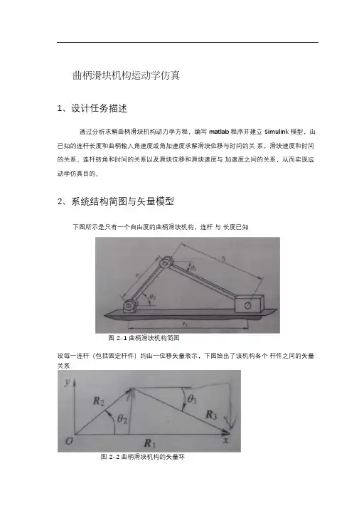
曲柄滑块机构运动学仿真1、设计任务描述通过分析求解曲柄滑块机构动力学方程,编写matlab 程序并建立Simulink 模型,由已知的连杆长度和曲柄输入角速度或角加速度求解滑块位移与时间的关系,滑块速度和时间的关系,连杆转角和时间的关系以及滑块位移和滑块速度与加速度之间的关系,从而实现运动学仿真目的。
2、系统结构简图与矢量模型下图所示是只有一个自由度的曲柄滑块机构,连杆与长度已知图2-1 曲柄滑块机构简图设每一连杆(包括固定杆件)均由一位移矢量表示,下图给出了该机构各个杆件之间的矢量关系图2-2 曲柄滑块机构的矢量环3.匀角速度输入时系统仿真3.1 系统动力学方程系统为匀角速度输入的时候,其输入为输出为;(1) 曲柄滑块机构闭环位移矢量方程为:(2) 曲柄滑块机构的位置方程(3) 曲柄滑块机构的运动学方程通过对位置方程进行求导,可得由于系统的输出是与,为了便于建立A*x=B 形式的矩阵,使x=[ ],将运动学方程两边进行整理,得到将上述方程的v1 与w3 提取出来,即可建立运动学方程的矩阵形式3.2 M 函数编写与Simulink 仿真模型建立3.2.1 滑块速度与时间的变化情况以及滑块位移与时间的变化情况仿真的基本思路:已知输入w2 与,由运动学方程求出w3 和v1,再通过积分,即可求出与r1。
(1) 编写Matlab 函数求解运动学方程将该机构的运动学方程的矩阵形式用M 函数compv(u)来表示。
设r2=15mm,r3=55mm,r1(0)=70mm,。
其中各个零时刻的初始值可以在Simulink 模型的积分器初始值里设置M 函数如下:function [x]=compv(u) %u(1)=w2%u(2)=sita2%u(3)=sita3 r2=15; r3=55;a=[r3*sin(u(3)) 1;-r3*cos(u(3)) 0]; b=[-r2*u(1)*sin(u(2));r2*u(1)*cos(u(2))]; x=inv(a)*b;2) 建立Simulink 模型M 函数创建完毕后,根据之前的运动学方程建立Simulink 模型,如下图:图3-1 Simulink 模型同时不要忘记设置r1 初始值70,如下图:图3-2 r1 初始值设置设置输入角速度为150rad/s ,运行时间为0.1s ,点击运行,即可从示波器中得到速度和时间以及位移和时间的图像3.2.2 滑块位移和滑块速度之间的图像为了得到滑块位移和滑块速度之间的图像,需要通过to workspace 模块将simulink 里位移和时间的数据传递到Matlab 的工作区中,从而在M 文件中再次利用,从Simulink 模块传递到工作区的数据的名称是simout。
电气学科大类Modern Control SystemsAnalysis and DesignUsing Matlab and Simulink Title: Automobile Velocity ControlName: 巫宇智Student ID: U200811997Class:电气0811电气0811 巫宇智CataloguePreface (3)The Design Introduction (4)Relative Knowledge (5)Design and Analyze (6)Compare and Conclusion (19)After design (20)Appendix (22)Reference (22)Automobile Velocity Control1.Preface:With the high pace of human civilization development, the car has been a common tools for people. However, some problems also arise in such tendency. Among many problems, the velocity control seems to a significant challenge.In a automated highway system, using the velocity control system to maintain the speed of the car can effectively reduce the potential danger of driving a car and also will bring much convenience to drivers.This article aims at the discussion about velocity control system and the compensator to ameliorate the preference of the plant, thus meets the complicated demands from people. The discussion is based on the simulation of MATLAB.Key word: PI controller, root locus电气0811 巫宇智2.The Design Introduction:Figure 2-1 automated highway systemThe figure shows an automated highway system, and according to computing and simulation, a velocity control system for maintaining the velocity if the two automobiles is developed as below.Figure 2-2 velocity control systemThe input, R(s), is the desired relative velocity between the twoAutomobile Velocity Controlvehicles. Our design goal is to develop a controller that can maintain the vehicles in several specification below.DS1 Zero steady-state error to a step inputDS2 Steady-state error due to a ramp input of less than 25% of the input magnitude.DS3 Percent overshoot less than 5% to a step input.DS4 Settling time less than 1.5 seconds to a step input( using a 2% criterion to establish settling time)3.Relative Knowledge:Controller here actually serves as a compensator, and we have some compensators for different specification and system.电气0811 巫宇智4.Design and Analysis:4.1S pecification analysisAccording to the relative knowledge above, I may consider a PI controller to compensate------------G c(s)=k p s+k I.sDs1: zero steady error to step response:To introduce an integral part to add the system type is enough.Ds2: Steady-state error due to a ramp input of less than 25% of the input magnitude.limsGc(s)G(s)≥4 −−→ Ki>4abs→0Ds3: overshoot less than 5% to a step response.P.0≤5% −−→ξ≥0.69DS4 Settling time less than 1.5 seconds to a step input( using a 2% criterion to establish settling time)Ts≤1.5 −−→ξ∗Wn≥2.66According to DS3 and DS4, we can draw the desired regionto placeAutomobile Velocity Controlour close-loop poles.(as the shadow indicate)Figure 4-1 Desired region for locating the dominant polesAfter adding the controller, the system transfer function become:T(s)=Kp s+Kis3+10s2+(16+Kp)s+KiThe corresponding Routh array is:s3 1 Kp+ab s2a+b Kis1ba KiabKpba+-++))((电气0811 巫宇智s0KiFor stability, we have (a+b)(Kp+ab)−Kia+b>0For another consideration, we need to put the break point of root locus to the shadow area in Figure 4-1 to ensure the dominant poles placed on the left of s=-2.66 line.a=−a−b−(−Ki Kp)2<−2.66In all, the specification is equal to a PI controller with limit below.{(a+b)(Kp+ab)−Kia+b>0⋯⋯⋯⋯⋯①KiKp<−5.32+(a+b)⋯⋯⋯⋯⋯⋯⋯②Ki>4ab⋯⋯⋯⋯⋯⋯⋯⋯⋯⋯⋯⋯③4.2Design process:4.2.1Controller verification:At the very beginning, we take the system with G(s)=1(s+2)(s+8)and the controller (provided by the book) withG c(s)=33+66sfor an initial discussion.Automobile Velocity ControlFigure 4-2 step response( a=2,b=8,Kp=33,Ki=66)Figure 4-3 ramp response( a=2,b=8,Kp=33,Ki=66)电气0811 巫宇智From figure 4-2, we can see that the overshoot is 4.75%, and the settling time is 1.04 s with zero error to the step input.From figure 4-3, it is clear that the ramp steady-state error is a little less than 25%.Thus, the controller with G c(s)=33+66scompletely meets the specification .4.2.2further analysis:For next procedure, I will have some more specific discussion about the applicable range of this controller to see how much can a and b vary yet allow the system to remain stable.We don’t change the parameter of the controller, and insert the Ki=66, Kp=33 into the inequality and get this:.{ab<16.5a+b>7.32ab+33−66a+b>0If we suppose the system to be a minimum phase system, a,b>0,thus it is easy to verify the 3rd inequality. Now, we draw to see the range of a and b.Figure4-4 the range of a,b for controller(Kp=33,Ki=66)Actually, the shade area can not completely meets the specification, for the constraint conditions represented in the 3 inequality is not enough, we need to draw the root locus for a certain system(a and b) to locate the actual limit for controller.However, this task is rather difficult, in a way, the 4 variables (a,b,Ki,Kp) all vary in terms of others’ change . Thus we can approximately locate the range of a and b from the figure above.4.2.3Alternatives discussion:According to inequality ①②③,The range of a and b bear some relation with the inequality below:{ a +b >5.32+Ki Kp ab <Ki 4Kp +ab −Ki a +b >0Basing our assumption on the range in the previous discussion, we can easily see that in order to increase the range, we can increase Ki and decrease the ratio of Ki to Kp.Thus, I adjust the parameter to{Ki =80Kp =64Figure4-5 the range of a,b for controller(Kp=64,Ki=80)As the figure indicate,(the range between dotted lines refers tothe previous controller, while the range between red lines refers to the new alternatives), the range increase as we expect.Next step, we may keep the system of G(s)=1(s+2)(s+8)fixed, and discuss the different compensating effect of different PI parameter.When carefully checking the controller, we may find that the controller actually add a zero( -Ki/Kp) , an integral part and a gain part, so we can only change the zero and draw the locus root and examine the step response and ramp response.KiKp=1.5:Figure4-6 the root locus (KiKp=1.5)Using rlocfind, we find the maximum Kp=34.8740So we choose 3 groups of parameter ([35,52.5],[30.45],[25,37.5]) to examine the reponseFigure4-7 the step response (KiKp=1.5)It’s clear that the step response preference is not satisfying with too long settling timeKiKp=2:Figure4-8 the root locus (KiKp=2)Using rlocfind, we find the maximum Kp=34.3673So we choose 3 groups of parameter to examine the response and ramp response.Figure4-9 the step response (KiKp=2)Figure4-10 the ramp response (KiKp=2)KiKp=2.5:Figure4-11 the root locus (KiKp=2.5)Using rlocfind, we find the maximum Kp=31.47Similarly, we choose 3 groups of parameter to examine the response and ramp response.Figure4-12 the step response (KiKp=2.5)Virtually, the overshoot (Kp=30, Ki=75) doesn’t meet thespecification as we expect. I guess, that may come from the effect ofzero(-2.5), thus , go back to the step response of KiKp=2, due to the elimination between zero(-2) and poles, thus the preference is within our expectation.Figure4-13 the ramp response (KiKp=2.5)pare and ConclusionMainly from the step response and ramp response, it can be concluded that, in a certain ratio of Ki to Kp, the larger Kp brings smaller ramp response error, as well as larger range of applicable system. Nevertheless, the larger Kp means worse step response preference(including overshoot and settling time).This contradiction is rather common in control system.In all, to get the most satisfying preference, we need to balanceall the parameter to make a compromise, but not a single parameter.From what we are talking about, we find the controller provided by the book(Kp=33, Ki=66) may be one of the best controller in comparison to some degree, with satisfying step response and ramp response preference, as well as a wider range for the variation of a and b, further, it use a zero(s=-2) to transfer the 3rd order system to 2nd order system, in doing so, we may eliminate some unexpected influence from the zero.The controller verified above (in Figure4-9 and Figure 4-10) with Kp=34, Kp=68 may be a little better, but only a little, and it doesn’t leave some margin.6.After Design这是一次艰难,且漫长的大作业,连续一个星期,每天忙到晚上3点,总算完成了这个设计,至少我自己是很满意的。

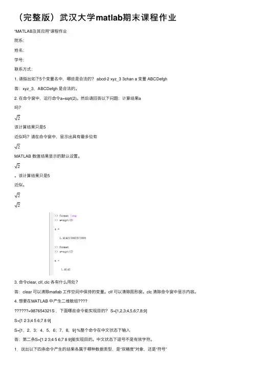
(完整版)武汉⼤学matlab期末课程作业“MATLAB及其应⽤”课程作业院系:姓名:学号:联系⽅式:1. 请指出如下5个变量名中,哪些是合法的? abcd-2 xyz_3 3chan a 变量 ABCDefgh答:xyz_3,ABCDefgh 是合法的。
2. 在命令窗中,运⾏命令a=sqrt(2)。
然后请回答以下问题:计算结果a吗?该计算结果只是5近似吗?请在命令窗中,显⽰出具有最多位有MATLAB 数值结果显⽰的默认设置。
该计算结果只是5近似。
3. 命令clear, clf, clc 各有什么⽤处?答:clear 可以清除matlab ⼯作空间中保持的变量。
clf 可以清除图形窗。
clc 清除命令窗中显⽰内容。
4. 想要在MATLAB 中产⽣⼆维数组=987654321S ,下⾯哪些命令能实现⽬的? S=[1,2,3;4,5,6;7,8;9]S=[1 2 3;4 5 6;7 8 9]S=[1,2,3;4,5,6;7,8,9] %整个命令在中⽂状态下输⼊答:第⼆条S=[1 2 3;4 5 6;7 8 9]能实现⽬的。
中⽂状态下逗号不是有效字符。
1.说出以下四条命令产⽣的结果各属于哪种数据类型,是“双精度”对象,还是“符号”对象?3/7+0.1, sym(3/7+0.1), vpa(sym(3/7+0.1),4), vpa(sym(3/7+0.1))答:3/7+0.1结果是双精度。
sym(3/7+0.1)结果是符号。
vpa(sym(3/7+0.1),4)结果是符号。
vpa(sym(3/7+0.1))结果是符号。
过程如图:2.已知a1=sin(sym(pi/4)+exp(sym(0.7)+sym(pi/3)))产⽣精准符号数字,请回答:以下产⽣的各种符号数哪些是精准的?若不精准,误差⼜是多少?能说出产⽣误差的原因吗?a2=sin(sym(pi/4)+exp(sym(0.7))*exp(sym(pi/3)))a3=sin(sym('pi/4')+exp(sym('0.7'))*exp(sym('pi/3')))a4=sin(sym('pi/4')+exp(sym('0.7+pi/3')))a5=sin(sym(pi/4)+exp(sym(0.7+pi/3)))a6=sin(sym(pi/4)+sym(exp(0.7+pi/3)))a7=sin(sym(pi/4+exp(0.7+pi/3)))a8=sym(sin(pi/4+exp(0.7+pi/3)))(提⽰:可⽤vpa观察误差;注意数位的设置)。
学习中心/函授站_ 成都学习中心姓名赵洪学号73西安电子科技大学网络与继续教育学院2015学年上学期《MATLAB与系统仿真》期末考试试题(综合大作业)考试说明:1、大作业于2015年4月3日公布,2015年5月9日前在线提交;2、考试必须独立完成,如发现抄袭、雷同、拷贝均按零分计。
3、程序设计题(三(8,10))要求写出完整的程序代码,并在matlab软件环境调试并运行通过,连同运行结果一并附上。
一、填空题(1’ ×25=25’)1、Matlab的全称为矩阵实验室。
2、在Matlab编辑器中运行程序的快捷键是:F5 。
3、Matlab的工作界面主要由以下五个部分组成,它们分别是:菜单栏、工具栏、当前工作目录窗口、工作空间管理窗口和命令窗口。
4、在Matlab中inf表示:无穷大;clc表示:清空命令窗口中的显示内容;more表示:在命令窗口中控制其后每页的显示内容行数;who表示:查阅Matlad内存变量名;whos表示:列出当前工作空间所有变量。
5、在Matlab命令窗口中运行命令Simulink 可以打开Simulink模块库浏览器窗口。
6、求矩阵行列式的函数:det ;求矩阵特征值和特征向量的函数eig 。
7、Matlab预定义变量ans表示:没有指定输出变量名;eps表示:系统精度;nargin表示:函数输入参数的个数。
8、Matlab提供了两种方法进行程序分析和优化,分别为:通过Profiler工具优化和通过tic和toc函数进行优化。
9、建立结构数组或转换结构数组的函数为:struct ;实现Fourier变换在Matlab中的对应函数为:fourier() ;Laplace变换的函数:Laplace() 。
10、MATLAB编写的程序文件称为M文件,M文件有脚本M文件和函数M文件两种。
二、简答题(3’×4=12’)1、简述MATLAB命令窗的主要作用?答:Matlab既可以运行命令也可以执行程序,在命令窗口中可以运行单独的命令也可以调用程序,相当方便,而编辑调试窗口和图像窗口都是程序运行结果展示窗口,可以很直观的对程序运行过程中出现的矩阵或者是变量等等进行监视。
《数字仿真及MATLAB》大作业指导书一、目的和任务配合《数字仿真及MATLAB》课程的理论教学,通过课程设计教学环节,使学生掌握当前流行的演算式MATLAB语言的基本知识,学会运用MATLAB 语言进行控制系统仿真和辅助设计的基本技能,有效地提高学生实验动手能力。
基本要求:1、利用MATLAB提供的基本工具,灵活地编制和开发程序,开创新的应用;2、熟练地掌握各种模型之间的转换,系统的时域、频域分析及根轨迹绘制;3、熟练运用SIMULINK对系统进行仿真;4、掌握PID控制器参数的设计。
二、设计要求1、编制相应的程序,并绘制相应的曲线;2、对设计结果进行分析;3、撰写和打印设计大作业报告(包括程序、结果分析、仿真结构框图、结果曲线)。
三、设计内容1、本次设计有三个可以选择的题目,选择一到两个题目进行设计;2、对于给定的系统模型,根据题目要求,设计控制器或对原系统进行校正,从而达到系统所要求的性能指标。
四、时间安排时间到考试前。
设计一:二阶弹簧—阻尼系统的PID 控制器设计及其参数整定考虑弹簧-阻尼系统如图1所示,其被控对象为二阶环节,传递函数G(S)如下,参数为M=1kg ,b=2N.s/m ,k=25N/m ,F (S )=1。
设计要求:(1) 控制器为P 控制器时,改变比例系数大小,分析其对系统性能的影响并绘制相应曲线。
(2) 控制器为PI 控制器时,改变积分时间常数大小,分析其对系统性能的影响并绘制相应曲线。
(例如当kp=50时,改变积分时间常数)(3) 设计PID 控制器,选定合适的控制器参数,使闭环系统阶跃响应曲线的超调量σ%<20%,过渡过程时间Ts<2s, 并绘制相应曲线。
图1 弹簧-阻尼系统示意图弹簧-阻尼系统的微分方程和传递函数为:F kx x b xM =++ 25211)()()(22++=++==s s k bs Ms s F s X s G图2 闭环控制系统结构图附:P 控制器的传递函数为:()P P G s K =PI 控制器的传递函数为:11()PI P I G s K T s=+⋅ PID 控制器的传递函数为:11()PID P D I G s K T s T s =+⋅+⋅设计二:二阶系统串联校正装置的设计与分析设某被控系统的传递函数G(s)如下:)2()(+=s s K s G 设计要求:选用合适的方法设计一个串联校正装置K(s),使闭环系统的阶跃响应曲线超调量%20%<σ,过渡过程时间.()s T 15s ≤,开环比例系数)/1(01s K v ≥,并分析串联校正装置中增益、极点和零点对系统性能的影响。
期末matlab考试题及答案注意:以下内容为虚构的期末MATLAB考试题目及答案,并非真实情况。
一、选择题1. 在MATLAB中,以下哪个命令可以将矩阵A的第一列元素求和?A) sum(A(:,1))B) sum(A(1,:))C) sum(A(1))D) sum(A(:,1))答案:A) sum(A(:,1))2. 对于向量x = [1, 2, 3, 4],以下哪个命令可以将x的元素逆序排列?A) flip(x)B) reverse(x)C) sort(x,'descend')D) sort(x,'ascend')答案:A) flip(x)3. 如果一个函数文件的文件名为"myFunction.m",那么在MATLAB中如何调用该函数?A) myFunction.mB) call myFunctionC) run myFunctionD) myFunction答案:D) myFunction4. 在MATLAB中,以下哪个命令可以生成一个在-1到1范围内均匀分布的10个数的向量?A) linspace(-1, 1, 10)B) rand(1, 10)*2-1C) linspace(1, 10, -1)D) randi([-1, 1], 1, 10)答案:B) rand(1, 10)*2-15. 对于矩阵A和B,以下哪个命令可以将它们进行垂直方向的拼接?A) vertcat(A, B)B) concat(A, B, 'vertical')C) merge(A, B, 'vertical')D) [A; B]答案:D) [A; B]二、填空题1. 假设有一个向量x = [1, 2, 3, 4],使用MATLAB命令求x的最大值。
答案:max(x)2. 假设有一个矩阵A = [1, 2, 3; 4, 5, 6; 7, 8, 9],使用MATLAB命令求A的行数。
M A T L A B大作业(总15页)--本页仅作为文档封面,使用时请直接删除即可----内页可以根据需求调整合适字体及大小--MATLAB大作业作业要求:(1)编写程序并上机实现,提交作业文档,包括打印稿(不含源程序)和电子稿(包含源程序),以班为单位交,作业提交截止时间6月24日。
(2)作业文档内容:问题描述、问题求解算法(方案)、MATLAB程序、结果分析、本课程学习体会、列出主要的参考文献。
打印稿不要求MATLAB程序,但电子稿要包含MATLAB程序。
(3)作业文档字数不限,但要求写实,写出自己的理解、收获和体会,有话则长,无话则短。
不要抄袭复制,可以参考网上、文献资料的内容,但要理解,要变成自己的语言,按自己的思路组织内容。
(4)从给出的问题中至少选择一题(多做不限,但必须独立完成,严禁抄袭)。
(5)大作业占过程考核的20%,从完成情况、工作量、作业文档方面评分。
第一类:绘制图形。
(B级)问题一:斐波那契(Fibonacci)螺旋线,也称黄金螺旋线(Golden spiral),是根据斐波那契数列画出来的螺旋曲线,自然界中存在许多斐波那契螺旋线的图案,是自然界最完美的经典黄金比例。
斐波那契螺旋线,以斐波那契数为边的正方形拼成的长方形,然后在正方形里面画一个90度的扇形,连起来的弧线就是斐波那契螺旋线,如图所示。
问题二:绘制谢尔宾斯基三角形(Sierpinskitriangle)是一种分形,由波兰数学家谢尔宾斯基在1915年提出,它是一种典型的自相似集。
其生成过程为:取一个实心的三角形(通常使用等边三角形),沿三边中点的连线,将它分成四个小三角形,然后去掉中间的那一个小三角形。
接下来对其余三个小三角形重复上述操作,如图所示。
问题三:其他分形曲线或图形。
分形曲线还有很多,教材介绍了科赫曲线,其他还有皮亚诺曲线、分形树、康托(G. Cantor)三分集、Julia集、曼德布罗集合(Mandelbrot set),等等。
1 / 7
MATLAB仿真
期末大作业
姓 名:班 级:学 号:指导教师:
2 / 7
2012春期末大作业
题目:设单位负反馈控制系统前向通道传递函数由)()(21sGsG和串联,其中:
)1(1)()(21sAsGs
K
sG
A表示自己学号最后一位数(可以是零),K为开环增益。要求:
(1)设K=1时,建立控制系统模型,并绘制阶跃响应曲线(用红色虚线,
并标注坐标和标题);求取时域性能指标,包括上升时间、超调量、调节时间、
峰值时间;
(2)在第(1)问中,如果是在命令窗口绘制阶跃响应曲线,用in1或者from
workspace模块将命令窗口的阶跃响应数据导入Simulink模型窗口,用示波器显
示阶跃响应曲线;如果是在Simulink模型窗口绘制阶跃响应曲线,用out1或者
to workspace模块将Simulink模型窗口的阶跃响应数据导入命令窗口并绘制阶跃
响应曲线。
(3)用编程法或者rltool法设计串联超前校正网络,要求系统在单位斜坡输
入信号作用时,速度误差系数小于等于0.1rad,开环系统截止频率sradc/4.4'',
相角裕度大于等于45度,幅值裕度大于等于10dB。
3 / 7
仿真结果及分析:
(1)、(2)、将Simulink模型窗口的阶跃响应数据导入命令窗口并绘制阶跃响应
曲线
通过在Matlab中输入命令:
>> plot(tout,yout,'r*-')
>> title('阶跃响应曲线')
即可得出系统阶跃响应曲线,如下:
求取该控制系统的常用性能指标:超调量、上升时间、调节时间、峰值时间的程
序如下:
G=zpk([],[0,-1],5)。
S=feedback(G,1)。
4 / 7
C=dcgain(S)。
[y,t]=step(S)。
plot(t,y)。
[Y,k]=max(y)。
timetopeak=t(k)。
percentovershoot=100*(Y-C)/C。
n=1。
while y(n)
end
ristime=t(n)。
i=length(t)。
while(y(i)>0.98*C)&(y(i)<1.02*C)
i=i-1。
end
setllingtime=t(i)。
运行程序得到如下结果:
Zero/pole/gain:
5
-------
s (s+1)
C=1(系统终值)
timetopeak=1.4365(峰值时间)
percentovershoot=8.0778(超调量)
ristime=0.8978(上升时间)
setllingtime=7.5415(调节时间)
(3)建立超前校正子函数如下:
function Gc=cqjz_frequency(G,kc,yPm)
G=tf(G)。
[mag,pha,w]=bode(G*kc)。
Mag=20*log10(mag)。
[Gm,Pm.Wcg,Wcp]=margin(G*kc)。
5 / 7
phi=(yPm-getfield(Pm,'Wcg'))*pi/180。
alpha=(1+sin(phi))/(1-sin(phi))。
Mn=-10*log(alpha)。
Wcgn=spline(Mag,w,Mn)。
T=1/Wcgn/sqrt(alpha)。
Tz=alpha*T。
Gc=tf([Tz,1],[T,1])。
主函数如下:
num=1。
den=conv([1,0],conv([0.3,1],[0.1,1]))。
G=tf(num,den)。
kc=6。yPm=45+6。
Gc=cqjz_frequency(G,kc,yPm)。
G=G*kc。
GGc=G*Gc。
Gy_close=feedback(G,1)。
Gx_close=feedback(GGc,1)。
figure(1)。
step(Gx_close,'b')。hold on。
step(Gy_close,'r')。grid
gtext('校正前的')。gtext('校正后的')。
figure(2)。
bode(G,'b')。
hold on。
bode(GGc,'r')。grid
gtext('校正前的')。gtext('校正后的')。gtext('校正前的')。gtext('校正后的')。
figure(3)。
nyquist(G,'b')。
hold on。
nyquist(GGc,'r')。grid
gtext('校正前的')。gtext('校正后的')。
绘制校正前后的单位阶跃响应曲线,开环伯德图和开环奈奎斯特曲线:
6 / 7
7 / 7