
中级宏观经济学_Ch01 The Science of Macroeconomics
- 格式:ppt
- 大小:6.63 MB
- 文档页数:12

《中级宏观经济学》教学大纲课程名称:中级宏观经济学课程英文名称:Intermediate Macroeconomics课内学时:32 课程学分:2课程性质(学位课/选修课)开课学期:每学年第一学期教学方式:课堂讲授,课堂讨论考核方式(考试/考查):考试大纲执笔人:熊苡主讲教师:熊苡师资队伍:熊苡、郭海涛一、课程内容简介中级宏观经济学作为一门产业经济学和金融学专业研究生的必修课或其他专业研究生的选修课,进一步从长期和短期、封闭和开放的角度分别对宏观经济的基本问题进行了研究。
主要内容包括对长期中经济增长、失业、通货膨胀问题的讨论;运用总需求—总供给模型和IS-LM模型解释短期经济波动,以及对总供给以及通货膨胀与失业的短期交替关系的进一步学习;结合模型分析开放的宏观经济学;介绍宏观经济政策争论和经济波动理论的进展。
二、课程目的和基本要求中级宏观经济学是在初级宏观经济学的基础上,对宏观经济问题进一步深入研究的经济学课程。
通过学习,要求学生在对宏观经济理论和经济模型了解和掌握的基础上,能够应用宏观经济学的原理和方法,对现实经济中的宏观经济政策及事件进行较为深入的分析。
本课程提倡学生广泛阅读、深入思考、展开讨论的教学方式,以达到在有限学时内教师精讲、学生宽学的目的。
通过学习,使学生对宏观经济学理论及方法有一个较为全面和深入的理解。
先修课程:初级微观经济学及初级宏观经济学。
三、课程主要内容1.导论(4学时)介绍宏观经济学的科学和宏观经济学的数据。
2.长期中的经济(8学时)主要内容有:(1)经济增长,介绍国民收入的基本古典模型;索洛增长模型;内生增长理论。
(2)失业的原因及形式;(3)货币与通货膨胀,运用古典货币理论的思想分析通货膨胀的原因与成本。
3.短期经济波动(8学时)主要内容有:(1)用总需求与总供给模型解释经济波动;(2)用IS-LM 模型解释经济波动;(3)总供给分析,四种总供给模型;通货膨胀、失业与菲利浦斯曲线。
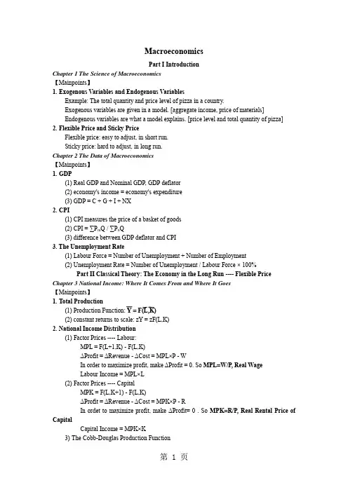
MacroeconomicsPart I IntroductionChapter 1 The Science of Macroeconomics【Mainpoints】1.Exogenous Variables and Endogenous VariablesExample: The total quantity and price level of pizza in a country.Exogenous variables are given in a model. [aggregate income, price of materials]Endogenous variables are what a model explains. [price level and total quantity of pizza]2.Flexible Price and Sticky PriceFlexible price: easy to adjust, in short run.Sticky price: hard to adjust, in long run.Chapter 2 The Data of Macroeconomics【Mainpoints】1.GDP(1) Real GDP and Nominal GDP, GDP deflator(2) economy's income = economy's expenditure(3) GDP = C + G + I + NX2.CPI(1) CPI measures the price of a basket of goods(2) CPI = ∑P m Q / ∑P n Q(3) difference between GDP deflator and CPI3. The Unemployment Rate(1) Labour Force = Number of Unemployment + Number of Employment(2) Unemployment Rate = Number of Unemployment / Labour Force × 100%Part II Classical Theory: The Economy in the Long Run ---- Flexible Price Chapter 3 National Income: Where It Comes From and Where It Goes【Mainpoints】1.Total Production(1) Production Function: Y = F(L,K)(2) constant returns to scale: zY = zF(L,K)2. National Income Distribution(1) Factor Prices ---- Labour:MPL = F(L+1,K) - F(L,K)ΔProfit = ΔRevenue - ΔCost = MPL×P - WIn order to maximize profit, make ΔProfit = 0. So MPL=W/P, Real WageLabour Income = MPL×L(2) Factor Prices ---- CapitalMPK = F(L,K+1) - F(L,K)ΔProfit = ΔRevenue - ΔCost = MPK×P - RIn ordet to maximize profit, make ΔProfit= 0 . So MPK=R/P, Real Rental Price of CapitalCapital Income = MPK×K3)The Cobb-Douglas Production FunctionLabour Income = MPL×L = (1-α)YCapital Income = MPK×K = αY→F(K,L) = AKαL(1-α) , A measures the productivity of the available technology3.Total Demand1)Consumption:Determined by disposable incomeC=C(Y-T)Marginal Propensity to ConsumeMPC=C(Y-T+1)-C(Y-T)2)Investment:Determined by interest rateI=I(r)When r is high, investors will give upinvestment because cost of loan is higherthan rate of return.3) Government PurchasesG vs T, measures government budget5. Equilibrium (in a closed economy)(1) Market of Goods and ServicesY=C(Y-T)+I(r)+G(2) Market of Loanable FundsS=Y-C(Y-T) - G = I(r)investment is crowded out Chapter 4 Money and Inflation【Mainpoints】1.Concept of Money(1) Funtions of Money: 1) Store of Value. Example: You can hold your money and trade itfor goods and services at some time in the future.2) Unit of Account. Example: In store people use money to showprice.3) Medium of Exchage. Example: People use money as tool toexchange goods.(2) Types of Money: 1) Fiat Money. No value, example: Paper Money.2) Commodity Money. With value, example: Gold and Silver.(3) Control of Money: 1) Institution: Central Bank. Example: Deutsche Bundesbank2) Method: Open-Markt Operation. Example: Buy governmentbonds to increase money supply.2.The Quantity Theory of Money(1) Quantity Equation: MV=PT →MV=PYQuantity Theory of Money: MV=PY(2) Real Money Balances: M/P , measured in quantity of goods and services.The Money Demand Function: (M/P)d = L(Y,i) = M/P← Money Supply. Y↑, d↑; i↑,d↓(3) Money and Inflation: ΔM% + ΔV% = ΔP% + ΔY% So M↑, P↑3.Inflation and Interest Rate(1) Fisher Equation: i = r + πChapter 5 The Open Economy【Mainpoints】1.International Trade in a Samll Open Economy(1) View of goods and capital flow: NX = Y- (C+G+I)(2) View of capital flow: NX = Y-C-G-I = S-I= S-I(r*)r* is World Interes Rate(3) Trade Policies: 1) Domestic Fiscal Policy, influenceG↑,T↓→S↓→NX↓2) Fiscal Policy Abroad, influenceG e↑, T e↓→S e↓→r*↑→NX↑3) Shift in investment demand. Example: Government provides aninvestment tax credit2.Exchange Rates(1) Nominal Exchange Rates(e) and Real Exchange Rates(ε)Nominal exchange rates are measured in currency. Example: 100 yen / 1 dollarReal exchage rates are measured in goods and services. Example: 2 Japan Car / 1 USA car ε = e × (P/P*) , P* means price level of foreign countries.(2) The Real Exchange Rates and Trade Balance:NX = NX(ε)ε↓, P/P*↓, mean s domestic goods and servicesare cheaper than abroad. NX↑When NX(ε) = S - I, ε is equilibrium real ex.rate.(3) Trade Policies: 1) Domestic Fiscal Policy:G↑,T↓ → S↓(Expansionary Fiscal Policy)2) Fiscal Policy Abroad:G e↑, T e↓→S e↓→r*↑→I↓3) Shift in investment demand.4) Shift in NX(ε) Example: Protectionist Trade Policies(4) Inflation and nominal exchange rates:e = ε × (P*/P) → Δe%= Δε% + (π* - π)(5) PPP(Purchasing-Power Parity): 1 Dollar can buy the same quantity of wheat in anycountry.Chapter 6 Unemployment【Mainpoints】1.Natual Rate of Unemployment(1) Concept: The rate of unemployment which the economy get closed to in the long run.(2) Calculation: L-Labour Froce, E-Number of Employed, U-Number of Unemployed, f-rate of job fiding, s-rate of job seperating.L=E+U, fU=sE → U/L=1/(1+f/s)2.Causes for Unemployment(1) Frictional Unemployment:Unemployed people need time to find jobs.e.g. sectoral shift, unemploymetn insurance.(2) Structural Unemployment:Wage Rigidity. Wage is above the equlibrium level.e.g. Minimum-Wage Laws, Unions, Efficiency Wages.Part III Growth Theory: The Economy in the Very Long Run ---- Solow Growth Model Chapter 7 Economic Growth I: Capital Accumulation and Population GrowthAssumption: Constant Return to Scale【Mainpoints】1.Capital Accumulation(1) Production Function per worker: zY=F(zK,zL)→Y/L=F(K/L,1)→y=f(k),MPK=f(k+1)-f(k)(2) Output and consumption per worker: y=c+i→c=(1-s)y→i=sy→i=sf(k)(3) The Steady State: Capital stock growth Δk = 0Δk=i-δk, δ is depreciation rate→Δk=sf(k)-δk=0→sf(k*)=δk*(4)Golden Rule level of capital: k*gold which maximizes cc=y-i→c=f(k)-sf(k)→c*=f(k*)-δk*→c max:MPK=δ2. Population Growth(at rate of n)(1) The Steady State:Δk=i-k(δ+n)→Δk=sf(k)-k(δ+n)=0→sf(k*)=(δ+n)k*(2) Golden Rule level of capital:k*gold, c=y-i→c max:MPK=δ+nChapter 8 Economic Growth I: Technology, Empirics, and Policy1.Technological Progress in the Solow ModelAssumption: Technology growth is a given exogenous variable g(1) Efficiency of Labour: Y=F(K,EL)(2) The Steady State: Δk=sf(k)-(g+n+δ)k=0→sf(k*)=(g+n+δ)k*(3) Golden Rule level of capital: k*gold , c=y-i→MPK=g+n+δ2.Endogenous Growth TheoryAssupmtion: Technolgy growth is a endogenous function g(μ), capital includes knowledge (1) 2 Sector Model: Y=F[K,(1-μ)EL], ΔE=g(μ)E, ΔK=sY-δKPart IV Business Cycle Theory: The Economy in the Short Run ---- Sticky Price Chapter 9 Introduction to Economic Fluctuations【Key Concepts】Recession: A period of falling output and rising unemployment.Business Cycle: Short-run fluctuations in output and employment.【Mainpoints】1.GDP and unemployment(1) Okun's Law: ΔReal GDP%=3%-2×ΔUnemployment Rate(2) Leading Economic Indicators: Forecasts. Example: Average work time, Index of stock prices, Money Supply....2.Aggregate Demand and Aggregate Supply( P=P(Y))(1) The Quantity Theory of Money→AD: MV=PY→M/P=(M/P)d=kY(2) AS: SRAS---P=P, LRAS---Y=Y(3) From Short Run to Long Run: M changes AD, Y is unchanged inthe long run, but P in the long run changes. (A→B→C)(4) Shocks to AD and AP:1) Shocks to AD. Example: Credit Card makes V rise.Policy: Reduce the Money Supply.2) Shocks to AP. Example: A drought that destroys crops. Cartel. Union. etc. P↑Policy: Wait! Then price returns original level eventually(But it takes longtime). Or expand AD(But price level will be high in long period of time) Chapter 10 Aggregate Demand I: Building the IS-LM Model (Y-r)【Mainpoints】1.IS Curve(1) Good and Service Market→The Keynesian Cross: Y=C+I+G, PE=AE(2) IS curve:Y=C(Y-T)+I(r)+G 1) r↑→I↓→Y↓ 2) Fiscal Policy: G↑→Y↑→IS→, Governmetn-purchases multiplier, tax multiplier.2.LM Curve(1) Money Market→The Theory of Liquidity Peference: M/ P=L(r), M s=M d(2) LM Curve: M/P=L(r,Y). 1) Y↑,M d↑,r↑ 2)M s↑,r↓,LM←3. The Short-Run EquilibriumChapter 11 Aggregate Demand II: Applying the IS-LM Model (Y-P)【Mainpoints】1.IS-LM Model as a Theroy of Aggregate Demand(1) Derivation: P↑,(M/P)s↓,r↑,LM↑→Y↓(2) Shift in AD: G,T,M→IS/LM→Y(3) In long run and short run: In long run Y<YChapter 12 The Open Economy Revisited: The Mundell-Fleming Model and the Exchange Rate Regime【Mainpoints】1.Mundell-Fleming Model(1) IS* Curve: Y=C(Y-T)+I(r*)+G+NX(ε) (2) LM* Curve: M/P=L(r*,Y)2.Under Floating Exchange Rates(1)Fiscal Policy:Shift IS*,ineffectual; Monetary Policy:Shift LM*; Trade Policy:Shift NX(ε)→IS* 3.Under Fixed Exchange Rates(1) Theory: Arbitrageur arbitrage so that M changes.(2)Fiscal Policy shifts IS*→LM*; Monetary Policy:Shift LM*, ineffectual; Trade Policy: Shift NX(ε)→IS*→LM*4. Policy Choice: Impossible Trinity5. Mundell-Fleming Model in Short andLong RunChapter 13 AS and the Short-Run Tradeoff Between Inflation and Unemployment1.Aggregate Supply ModelY=Y+α(P-P e)2.Inflation, Unemployment and Phillips Curve(1)Y=Y+α(P-P e)→P-P-1=P e-P-1+1/α(Y-Y)+v→π=πe+β(μ-μn)+v [Okun's Law] v-supply shock(2) Sacrifice Ratio: π↓1%, GDP ↓ ? %Part V Macroeconomic Policy DebateChapter 14 Stabilization Policy1.Inside Lag and Outside Lag(1) Inside lag is the time between economy shock and the policy anction responds. Example: Policy makers need time to recognize a shock and react.(2) Outside lag is the time between a policy action and its influence on the economy. Example: Change in money supply and interest rate.Chapter 15 Government Debt and Budget Deficits1.The Traditional View of Government Debt(1) In the short run, T↓,C↑,S↓,r↑,I↓,lower steady-state K and a lower level of Y.(2) In the lo ng run, T↓,C↑,IS→,AD↑, finally Y=Y, P i s higher.(3) In open economy, T↓,C↑,IS→, ε↑2.The Ricardian View of Government Debt(1) Ricardian Equivalence: Consumers are forward-looking.They think that government will raise tax at some point in the future, in order to afford budget. So they won't change consumption.Part VI More on the Microeconomics Behind MacroeconomicsChapter 18 Money Supply, Money Demand and the Banking System1.Money Supply(1) Money Supply (M) = Currency (C) + Demand Deposits (D)(2) Reserves: The money that bank receive but don't lend out. Reserve-deposit ratio-rr1) 100% Reserve Banking. 1C→1D, M remains constant.2) Fractional-Reserve Banking. 1C→rrD+(1-rr)C, M increases. And (1-rr)C can be put into another bank, the process of money creation can be continued.(3) Money Supply Model: M=C+D.B(Monetary Base)=C+R [Control by Central Bank]→ M=(cr+1)/(cr+rr)×B=m×B [cr is currency-deposit ratio](4) Monetary Policy Tool: open-market operation, reserve requirements, discout rate[the rate that banks borrow from central bank].2.Money Demand(1) Quantity Theory: (M/P)d=L(i;Y)(2) Portfolio Theory: (M/P)d=L(r s,r b,πe,W) [r s-expected real return on stock, r b-expected real return on bonds, W-real wealth]。

中级宏观经济学课程教学⼤纲《中级宏观经济学》课程教学⼤纲⼀、课程名称中级宏观经济学Intermediate Macroeconomics⼆、课程编码:三、学时与学分:64/4四、先修课程:《中级微观经济学》或《经济学原理》、⾼等数学五、课程教学⽬标:1.介绍⼀些宏观经济现象与事实;了解宏观经济学家所关⼼的主要问题及其分析⽅法;2.引导学⽣建⽴宏观经济模型,理解导致经济长期增长和短期波动的根源;3.理解宏观经济学家和政策制订者通过政府政策来影响宏观经济的效果。
六、适⽤学科专业经济学、⾦融学、财政学、国际贸易七、基本教学内容与学时安排1.导论篇:8学时了解宏观经济学研究的对象、⽅法和⽬标了解宏观经济学的核⼼变量及其度量⽅法了解宏观经济学的国民会计⽅程2.长期篇:12学时了解宏观经济学中的总产出、收⼊分配及产品市场的均衡是如何决定的了解通货膨胀的成因、影响及社会成本了解⾃然失业率的含义、成因及其背后的决定因素了解⼩开放经济模型的含义及政策对开放经济的影响3.增长篇:10学时了解索洛模型中稳态的含义、黄⾦稳态的决定和向稳态的调整过程了解技术进步对长期经济增长的意义、长期增长的源泉和⼈⼒资本的重要性了解储蓄率、⼈⼝出⽣率等变量对稳态的影响及相关政策含义能解释美国新经济现象,并为不同国家的发展政策提供政策建议4.波动篇:16学时了解短期波动与长期增长在模型⽅法上的异同了解凯恩斯学派对宏观经济波动的解释及其政策主张了解IS-LM模型的含义及其在政策分析中的作⽤了解IS-LM模型到AS-AD模型的推导及其在政策分析中的作⽤能将IS-LM模型推⼴到开放经济并掌握蒙代尔-弗莱明模型的含义了解粘性⼯资、粘性价格和不完全信息三个总供给模型及菲利普斯曲线、奥肯定律和牺牲率等概念了解真实商业周期理论的模型思路、政策主张、主要结论和动态随机⼀般均衡⽅法5.政策篇:8学时了解政府预算、财政政策和李嘉图-巴罗等价命题的政策含义了解货币政策规则了解理性预期学派、货币主义学派和凯恩斯学派的政策主张6.基础篇:8学时了解消费理论的发展演变过程及其核⼼思想了解投资理论的发展演变过程及现代投资理论的进展了解货币需求理论的微观基础及货币供给的⽣成过程7.中国篇:2学时了解中国⾃改⾰开放以来宏观经济的表现及政府政策的效果评价⼋、教材及参考书教材:N. G. Mankiw. Macroeconomics. 5ed. Worth Publishers, 2002.主要参考书:Rudiger Dornbusch, Stanley Fisher, and Richard Startz. Macroeconomics. McGraw-Hill, 2001;Andrew B. Abel and Ben S. Bernanke. Macroeconomics. Addison-Wesley Publishing Co., 1995;William Branson. Macroeconomic Theory and Policy. Addison-Wesley Publishing Co., 1989.九、考核⽅式期末考试:60%平时作业:30%课堂表现:10%。