CR Categories and Subject Descriptors D1.5 [Software] Programming

A Simple Min-Cut AlgorithmMECHTHILD STOERTeleverkets Forskningsinstitutt,Kjeller,NorwayANDFRANK WAGNERFreie Universita¨t Berlin,Berlin-Dahlem,GermanyAbstract.We present an algorithm for finding the minimum cut of an undirected edge-weighted graph.It is simple in every respect.It has a short and compact description,is easy to implement,and has a surprisingly simple proof of correctness.Its runtime matches that of the fastest algorithm known.The runtime analysis is straightforward.In contrast to nearly all approaches so far,the algorithm uses no flow techniques.Roughly speaking,the algorithm consists of about͉V͉nearly identical phases each of which is a maximum adjacency search.Categories and Subject Descriptors:G.L.2[Discrete Mathematics]:Graph Theory—graph algorithms General Terms:AlgorithmsAdditional Key Words and Phrases:Min-Cut1.IntroductionGraph connectivity is one of the classical subjects in graph theory,and has many practical applications,for example,in chip and circuit design,reliability of communication networks,transportation planning,and cluster analysis.Finding the minimum cut of an undirected edge-weighted graph is a fundamental algorithmical problem.Precisely,it consists in finding a nontrivial partition of the graphs vertex set V into two parts such that the cut weight,the sum of the weights of the edges connecting the two parts,is minimum.A preliminary version of this paper appeared in Proceedings of the2nd Annual European Symposium on Algorithms.Lecture Notes in Computer Science,vol.855,1994,pp.141–147.This work was supported by the ESPRIT BRA Project ALCOM II.Authors’addresses:M.Stoer,Televerkets Forskningsinstitutt,Postboks83,2007Kjeller,Norway; e-mail:mechthild.stoer@nta.no.;F.Wagner,Institut fu¨r Informatik,Fachbereich Mathematik und Informatik,Freie Universita¨t Berlin,Takustraße9,Berlin-Dahlem,Germany;e-mail:wagner@inf.fu-berlin.de.Permission to make digital/hard copy of part or all of this work for personal or classroom use is granted without fee provided that the copies are not made or distributed for profit or commercial advantage,the copyright notice,the title of the publication,and its date appear,and notice is given that copying is by permission of the Association for Computing Machinery(ACM),Inc.To copy otherwise,to republish,to post on servers,or to redistribute to lists,requires prior specific permission and/or a fee.᭧1997ACM0004-5411/97/0700-0585$03.50Journal of the ACM,Vol.44,No.4,July1997,pp.585–591.586M.STOER AND F.WAGNER The usual approach to solve this problem is to use its close relationship to the maximum flow problem.The famous Max-Flow-Min-Cut-Theorem by Ford and Fulkerson[1956]showed the duality of the maximum flow and the so-called minimum s-t-cut.There,s and t are two vertices that are the source and the sink in the flow problem and have to be separated by the cut,that is,they have to lie in different parts of the partition.Until recently all cut algorithms were essentially flow algorithms using this duality.Finding a minimum cut without specified vertices to be separated can be done by finding minimum s-t-cuts for a fixed vertex s and all͉V͉Ϫ1possible choices of tʦVگ{s}and then selecting the lightest one.Recently Hao and Orlin[1992]showed how to use the maximum flow algorithm by Goldberg and Tarjan[1988]in order to solve the minimum cut problem in timeᏻ(͉VʈE͉log(͉V͉2/͉E͉),which is nearly as fast as the fastest maximum flow algorithms so far[Alon1990;Ahuja et al.1989;Cheriyan et al. 1990].Nagamochi and Ibaraki[1992a]published the first deterministic minimum cut algorithm that is not based on a flow algorithm,has the slightly better running time ofᏻ(͉VʈE͉ϩ͉V͉2log͉V͉),but is still rather complicated.In the unweighted case,they use a fast-search technique to decompose a graph’s edge set E into subsets E1,...,E␭such that the union of the first k E i’s is a k-edge-connected spanning subgraph of the given graph and has at most k͉V͉edges.They simulate this approach in the weighted case.Their work is one of a small number of papers treating questions of graph connectivity by non-flow-based methods [Nishizeki and Poljak1989;Nagamochi and Ibaraki1992a;Matula1992].Karger and Stein[1993]suggest a randomized algorithm that with high probability finds a minimum cut in timeᏻ(͉V͉2log͉V͉).In this context,we present in this paper a remarkably simple deterministic minimum cut algorithm with the fastest running time so far,established in Nagamochi and Ibaraki[1992b].We reduce the complexity of the algorithm of Nagamochi and Ibaraki by avoiding the unnecessary simulated decomposition of the edge set.This enables us to give a comparably straightforward proof of correctness avoiding,for example,the distinction between the unweighted, integer-,rational-,and real-weighted case.This algorithm was found independently by Frank[1994].Queyranne[1995]generalizes our simple approach to the minimization of submodular functions.The algorithm described in this paper was implemented by Kurt Mehlhorn from the Max-Planck-Institut,Saarbru¨cken and is part of the algorithms library LEDA[Mehlhorn and Na¨her1995].2.The AlgorithmThroughout the paper,we deal with an ordinary undirected graph G with vertex set V and edge set E.Every edge e has nonnegative real weight w(e).The simple key observation is that,if we know how to find two vertices s and t, and the weight of a minimum s-t-cut,we are nearly done:T HEOREM2.1.Let s and t be two vertices of a graph G.Let G/{s,t}be the graph obtained by merging s and t.Then a minimum cut of G can be obtained by taking the smaller of a minimum s-t-cut of G and a minimum cut of G/{s,t}.The theorem holds since either there is a minimum cut of G that separates s and t ,then a minimum s -t -cut of G is a minimum cut of G ;or there is none,then a minimum cut of G /{s ,t }does the job.So a procedure finding an arbitrary minimum s -t -cut can be used to construct a recursive algorithm to find a minimum cut of a graph.The following algorithm,known in the literature as maximum adjacency search or maximum cardinality search ,yields the desired s -t -cut.M INIMUM C UT P HASE (G ,w ,a )A 4{a }while A Vadd to A the most tightly connected vertexstore the cut-of-the-phase and shrink G by merging the two vertices added lastA subset A of the graphs vertices grows starting with an arbitrary single vertex until A is equal to V .In each step,the vertex outside of A most tightly connected with A is added.Formally,we add a vertexz ʦ͞A such that w ͑A ,z ͒ϭmax ͕w ͑A ,y ͉͒y ʦ͞A ͖,where w (A ,y )is the sum of the weights of all the edges between A and y .At the end of each such phase,the two vertices added last are merged ,that is,the two vertices are replaced by a new vertex,and any edges from the two vertices to a remaining vertex are replaced by an edge weighted by the sum of the weights of the previous two edges.Edges joining the merged nodes are removed.The cut of V that separates the vertex added last from the rest of the graph is called the cut-of-the-phase .The lightest of these cuts-of-the-phase is the result of the algorithm,the desired minimum cut:M INIMUM C UT (G ,w ,a )while ͉V ͉Ͼ1M INIMUM C UT P HASE (G ,w ,a )if the cut-of-the-phase is lighter than the current minimum cutthen store the cut-of-the-phase as the current minimum cutNotice that the starting vertex a stays the same throughout the whole algorithm.It can be selected arbitrarily in each phase instead.3.CorrectnessIn order to proof the correctness of our algorithms,we need to show the following somewhat surprising lemma.L EMMA 3.1.Each cut -of -the -phase is a minimum s -t -cut in the current graph ,where s and t are the two vertices added last in the phase .P ROOF .The run of a M INIMUM C UT P HASE orders the vertices of the current graph linearly,starting with a and ending with s and t ,according to their order of addition to A .Now we look at an arbitrary s -t -cut C of the current graph and show,that it is at least as heavy as the cut-of-the-phase.587A Simple Min-Cut Algorithm588M.STOER AND F.WAGNER We call a vertex v a active(with respect to C)when v and the vertex added just before v are in the two different parts of C.Let w(C)be the weight of C,A v the set of all vertices added before v(excluding v),C v the cut of A vഫ{v} induced by C,and w(C v)the weight of the induced cut.We show that for every active vertex vw͑A v,v͒Յw͑C v͒by induction on the set of active vertices:For the first active vertex,the inequality is satisfied with equality.Let the inequality be true for all active vertices added up to the active vertex v,and let u be the next active vertex that is added.Then we havew͑A u,u͒ϭw͑A v,u͒ϩw͑A uگA v,u͒ϭ:␣Now,w(A v,u)Յw(A v,v)as v was chosen as the vertex most tightly connected with A v.By induction w(A v,v)Յw(C v).All edges between A uگA v and u connect the different parts of C.Thus they contribute to w(C u)but not to w(C v).So␣Յw͑C v͒ϩw͑A uگA v,u͒Յw͑C u͒As t is always an active vertex with respect to C we can conclude that w(A t,t)Յw(C t)which says exactly that the cut-of-the-phase is at most as heavy as C.4.Running TimeAs the running time of the algorithm M INIMUM C UT is essentially equal to the added running time of the͉V͉Ϫ1runs of M INIMUM C UT P HASE,which is called on graphs with decreasing number of vertices and edges,it suffices to show that a single M INIMUM C UT P HASE needs at mostᏻ(͉E͉ϩ͉V͉log͉V͉)time yielding an overall running time ofᏻ(͉VʈE͉ϩ͉V͉2log͉V͉).The key to implementing a phase efficiently is to make it easy to select the next vertex to be added to the set A,the most tightly connected vertex.During execution of a phase,all vertices that are not in A reside in a priority queue based on a key field.The key of a vertex v is the sum of the weights of the edges connecting it to the current A,that is,w(A,v).Whenever a vertex v is added to A we have to perform an update of the queue.v has to be deleted from the queue,and the key of every vertex w not in A,connected to v has to be increased by the weight of the edge v w,if it exists.As this is done exactly once for every edge,overall we have to perform͉V͉E XTRACT M AX and͉E͉I NCREASE K EY ing Fibonacci heaps[Fredman and Tarjun1987],we can perform an E XTRACT M AX operation inᏻ(log͉V͉)amortized time and an I NCREASE K EY operation inᏻ(1)amortized time.Thus,the time we need for this key step that dominates the rest of the phase, isᏻ(͉E͉ϩ͉V͉log͉V͉).5.AnExample F IG .1.A graph G ϭ(V ,E )withedge-weights.F IG .2.The graph after the first M INIMUM C UT P HASE (G ,w ,a ),a ϭ2,and the induced ordering a ,b ,c ,d ,e ,f ,s ,t of the vertices.The first cut-of-the-phase corresponds to the partition {1},{2,3,4,5,6,7,8}of V with weight w ϭ5.F IG .3.The graph after the second M INIMUM C UT P HASE (G ,w ,a ),and the induced ordering a ,b ,c ,d ,e ,s ,t of the vertices.The second cut-of-the-phase corresponds to the partition {8},{1,2,3,4,5,6,7}of V with weight w ϭ5.F IG .4.After the third M INIMUM C UT P HASE (G ,w ,a ).The third cut-of-the-phase corresponds to the partition {7,8},{1,2,3,4,5,6}of V with weight w ϭ7.589A Simple Min-Cut AlgorithmACKNOWLEDGMENT .The authors thank Dorothea Wagner for her helpful re-marks.REFERENCESA HUJA ,R.K.,O RLIN ,J.B.,AND T ARJAN ,R.E.1989.Improved time bounds for the maximum flow problem.SIAM put.18,939–954.A LON ,N.1990.Generating pseudo-random permutations and maximum flow algorithms.Inf.Proc.Lett.35,201–204.C HERIYAN ,J.,H AGERUP ,T.,AND M EHLHORN ,K.1990.Can a maximum flow be computed in o (nm )time?In Proceedings of the 17th International Colloquium on Automata,Languages and Programming .pp.235–248.F ORD ,L.R.,AND F ULKERSON ,D.R.1956.Maximal flow through a network.Can.J.Math.8,399–404.F RANK , A.1994.On the Edge-Connectivity Algorithm of Nagamochi and Ibaraki .Laboratoire Artemis,IMAG,Universite ´J.Fourier,Grenoble,Switzerland.F REDMAN ,M.L.,AND T ARJAN ,R.E.1987.Fibonacci heaps and their uses in improved network optimization algorithms.J.ACM 34,3(July),596–615.G OLDBERG ,A.V.,AND T ARJAN ,R.E.1988.A new approach to the maximum-flow problem.J.ACM 35,4(Oct.),921–940.H AO ,J.,AND O RLIN ,J.B.1992.A faster algorithm for finding the minimum cut in a graph.In Proceedings of the 3rd ACM-SIAM Symposium on Discrete Algorithms (Orlando,Fla.,Jan.27–29).ACM,New York,pp.165–174.K ARGER ,D.,AND S TEIN ,C.1993.An O˜(n 2)algorithm for minimum cuts.In Proceedings of the 25th ACM Symposium on the Theory of Computing (San Diego,Calif.,May 16–18).ACM,New York,pp.757–765.F IG .5.After the fourth and fifth M INIMUM C UT P HASE (G ,w ,a ),respectively.The fourth cut-of-the-phase corresponds to the partition {4,7,8},{1,2,3,5,6}.The fifth cut-of-the-phase corresponds to the partition {3,4,7,8},{1,2,5,6}with weight w ϭ4.F IG .6.After the sixth and seventh M INIMUM C UT P HASE (G ,w ,a ),respectively.The sixth cut-of-the-phase corresponds to the partition {1,5},{2,3,4,6,7,8}with weight w ϭ7.The last cut-of-the-phase corresponds to the partition {2},V گ{2};its weight is w ϭ9.The minimum cut of the graph G is the fifth cut-of-the-phase and the weight is w ϭ4.590M.STOER AND F.WAGNERM ATULA ,D.W.1993.A linear time 2ϩ⑀approximation algorithm for edge connectivity.In Proceedings of the 4th ACM–SIAM Symposium on Discrete Mathematics ACM,New York,pp.500–504.M EHLHORN ,K.,AND N ¨AHER ,S.1995.LEDA:a platform for combinatorial and geometric mun.ACM 38,96–102.N AGAMOCHI ,H.,AND I BARAKI ,T.1992a.Linear time algorithms for finding a sparse k -connected spanning subgraph of a k -connected graph.Algorithmica 7,583–596.N AGAMOCHI ,H.,AND I BARAKI ,puting edge-connectivity in multigraphs and capaci-tated graphs.SIAM J.Disc.Math.5,54–66.N ISHIZEKI ,T.,AND P OLJAK ,S.1989.Highly connected factors with a small number of edges.Preprint.Q UEYRANNE ,M.1995.A combinatorial algorithm for minimizing symmetric submodular functions.In Proceedings of the 6th ACM–SIAM Symposium on Discrete Mathematics ACM,New York,pp.98–101.RECEIVED APRIL 1995;REVISED FEBRUARY 1997;ACCEPTED JUNE 1997Journal of the ACM,Vol.44,No.4,July 1997.591A Simple Min-Cut Algorithm。

Package‘INSPIRE’October12,2022Type PackageTitle Inferring Shared Modules from Multiple Gene Expression Datasetswith Partially Overlapping Gene SetsVersion1.5Date2016-12-08Author Safiye CelikMaintainer Safiye Celik<********************.edu>Description A method to infer modules of co-expressed genes and thedependencies among the modules from multiple expression datasets that maycontain different sets of genes.Please refer to:Extracting a low-dimensionaldescription of multiple gene expression datasets reveals a potential driver fortumor-associated stroma in ovarian cancer,Safiye Celik,Benjamin A.Logsdon,Stephanie Battle,Charles W.Drescher,Mara Rendi,R.David Hawkins and Su-InLee(2016)<DOI:10.1186/s13073-016-0319-7>.License GPL(>=2)URL Imports missMDARoxygenNote5.0.1NeedsCompilation yesRepository CRANDate/Publication2016-12-0922:52:45R topics documented:exmp_dataset1 (2)exmp_dataset2 (2)INSPIRE (2)Index41exmp_dataset1Example Gene Expression Dataset-1DescriptionThis example ovarian cancer dataset contains expression of random half of the genes on the28 samples from the GSE19829.GPL570accession in Gene Expression Omnibus.Contains28sam-ples(as rows)and9056genes(as columns).4117of the genes are overlapping with the genes in exmp_dataset2.exmp_dataset2Example Gene Expression Dataset-2DescriptionThis example ovarian cancer dataset contains expression of random half of the genes on the42 samples from the GSE19829.GPL8300accession in Gene Expression Omnibus.Contains42sam-ples(as rows)and4165genes(as columns).4117of the genes are overlapping with the genes in exmp_dataset1.INSPIRE Inferring Shared Modules from Multiple Gene Expression Datasetswith Partially Overlapping Gene SetsDescriptionTakes a list of data matrices,with potentially different number of genes,number of modules,anda penalty parameter,and returns thefinal assignment of the data points in each dataset to the mod-ules,the values of the module latent variables,and the conditional dependency network among the module latent variables.UsageINSPIRE(datasetlist,mcnt,lambda,printoutput=0,maxinitKMiter=100,maxiter=100,threshold=0.01,initseed=123)Argumentsdatasetlist A list of gene expression matrices of size n_i x p_i where rows represent samples and columns represent genes for each dataset i.This can be created by using thelist()command,e.g.,list(dataset1,dataset2,dataset3)mcnt A positive integer representing the number of modules to learn from the data lambda A penalty parameter that regularizes the estimated precision matrix representing the conditional dependencies among the modulesprintoutput0or1representing whether the progress of the algorithm should be displayed(0 means no display which is the default)maxinitKMiter Maximum number of K-means iterations performed to initialize the parameters (the default is100iterations)maxiter Maximum number of INSPIRE iterations performed to update the parameters (the default is100iterations)threshold Convergence threshold measured as the relative change in the sum of the el-ements of the estimated precision matrices in two consecutive iterations(thedefault is10^-2)initseed The random seed set right before the K-means call which is performed to ini-tialize the parametersValueL A matrix of size(sum_n_i)x mcnt representing the inferred latent variables(the low-dimensional representation-or LDR-of the data)Z A list of vectors of size p_i representing the learned assignment of each of the genes in each dataset i to one of mcnt modulestheta Estimated precision matrix of size mcnt x mcnt representing the conditional dependencies among the modulesExamples##Not run:library(INSPIRE)mcnt=90#module sizelambda=.1#penalty parameter to induce sparsity#download two real gene expression datasets,where the rows are genes and columns are samples data( two_example_datasets )#log-normalize,and standardize each datasetres=INSPIRE(list(scale(log(exmp_dataset1)),scale(log(exmp_dataset2))),mcnt,lambda) ##End(Not run)Indexexmp_dataset1,2exmp_dataset2,2INSPIRE,24。

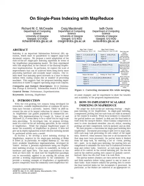
On Single-Pass Indexing with MapReduceRichard M.C.McCreadie Department of ComputingScienceUniversity of GlasgowGlasgow,G128QQ richardm@Craig MacdonaldDepartment of ComputingScienceUniversity of GlasgowGlasgow,G128QQcraigm@Iadh OunisDepartment of ComputingScienceUniversity of GlasgowGlasgow,G128QQounis@ABSTRACTIndexing is an important Information Retrieval(IR)op-eration,which must be parallelised to support large-scale document corpora.We propose a novel adaptation of the state-of-the-art single-pass indexing algorithm in terms of the MapReduce programming model.We then experiment with this adaptation,in the context of the Hadoop MapRe-duce implementation.In particular,we explore the scale of improvements that can be achieved when usingfirstly more processing hardware and secondly larger corpora.Our re-sults show that indexing speed increases in a close to linear fashion when scaling corpus size or number of processing machines.This suggests that the proposed indexing imple-mentation is viable to support upcoming large-scale corpora. Categories and Subject Descriptors:H.3.3[Informa-tion Storage&Retrieval]:Information Search&Retrieval General Terms:Performance,Experimentation Keywords:Indexing,MapReduce1.INTRODUCTIONWith the ever-growing test corpora being developed for researchers,scalable implementations of common IR opera-tions have become a necessity.Indeed,TREC in2009in-creased the size of its largest collection by almost12times. As MapReduce has gained popularity in commercial set-tings,with implementations by Google[3],Yahoo![2]and Microsoft[5],it seems likely to be a viable tool for large-scale data processing.To investigate this,we propose develop-ment of a state-of-the-art indexing operation,in the context of MapReduce.While the original MapReduce paper[3] shows the scalability of MapReduce in general,it does not give an in-depth explanation of how efficient indexing should be performed within such a model.In Section2,we develop a novel indexing strategy in MapReduce,inspired by the single-pass indexing of Heinz &Zobel[4].In particular,we employ Hadoop[2]-the only freely available MapReduce implementation,developed by Yahoo!.Section3,presents experiments using our MapRe-duce indexing strategy,to assess its scalability,in terms of hardware and input data.The main contributions of this work are three-fold:we show how the MapReduce paradigm can be successfully applied to an existing IR system and provide a working implementation to the community;we provide a working example of MapReduce of significantly greater complexity than the commonly-used MapReduce wo-Copyright is held by the author/owner(s).SIGIR’09,July19–23,2009,Boston,Massachusetts,USA.ACM978-1-60558-483-6/09/07.Figure1:Correcting document IDs while merging. rd count example;and we experiment to show the benefits and scalability of the proposed implementation.2.HOW-TO IMPLEMENT SCALABLEINDEXING IN MAPREDUCEWe adapt the state-of-the-art indexing strategy-single-pass indexing[4]for MapReduce.In single-pass indexing, (compressed)posting lists for each term are built in memory as the corpus is scanned.When local memory is exhausted, the partial indices are‘flushed’to disk and thefinal index is built from the mergedflushes.Elias-Gamma compression is used to store document-identifier(doc-id)deltas,ensuring postings are fully compressed,both in memory and on disk. We now propose a conversion for single-pass indexing into MapReduce.Document processing is split over m map tasks, with each map task processing its own subset of the input data.However,when memory runs low or all documents for that map have been processed,the partial index isflushed from the map task,by emitting a set of<term,posting list>pairs.As in single-pass indexing,the posting lists are compressed to minimise the data that is transferred between map and reduce tasks.Moreover,as each map task is not aware of its context in the overall indexing job,the doc-ids used in the emitted posting lists cannot be globally correct. Instead,these doc-ids start from0in eachflush.The partial indices(flushes)are then sorted by term,map andflush numbers before being passed to one or more re-duce tasks.Each reducer collates the posting lists to create thefinal inverted index for the documents it processed.In particular,as theflushes are collected at an appropriate re-duce task,the posting lists for each term are merged by map number andflush number,to ensure that the posting lists for each term are in a globally correct doc-id ordering. The reduce function takes each term in turn and merges the posting lists for that term into a full posting list.Figure1 presents an example for a distributed setting MapReduce indexing paradigm of200documents.Note that the num-ber of reduce tasks therefore determines thefinal number ofinverted index shards created.3.EXPERIMENTATION&RESULTSTo determine the extent to which MapReduce is a suitable framework for efficiently processing large IR corpora,we in-vestigate two research questions:does our Hadoop MapRe-duce implementation attain linear speedup with machines allocated(i.e.doubling machines would ideally half index-ing time);and how does corpora size affect performance? Our indexer uses the Hadoop MapReduce implementation (v.0.18.2)and we evaluate using four standard TREC cor-pora of varying size,namely WT2G,WT10G,.GOV and .GOV2.Of these,.GOV2is the largest at25M documents, comprising425GB when uncompressed.Firstly,we test to determine if the distributed(MapRe-duce)indexing will complete the same indexing process in a shorter time as we increase the processing power available. To show this,we measure the mean indexing time 2 (5repetitions),running on1-8machines,when using a sin-gle reduce task.From the single reducer curve in Figure2, we observe that indexing time decreases as more machines are added(i.e.speedup increases).However,by examining the trends observed as the number of machines increases, we see that linear speedup is not achieved,as indexing time speedups level offafter approximately6machines.On further analysis,we suggest that this is due to the use of a single reduce task,with this becoming the bottleneck of the indexing job,i.e.the(sequential)single reduce task lim-its the speedup achievable as described in Amdahl’s law[1]. To test this,we then experimented indexing when using24 reducers.The results are presented in the multiple reducer curve in Figure2.Indeed,this shows that by using multi-ple reduce tasks we achieve marked performance improve-ments beyond6machines.As an illustration to this success, we note that the single-pass(single-threaded)indexing took over a day(1605minutes)to 2.However,when running the multi-threaded MapReduce implementation on a single three-core machine,indexing completed in less than 8hours(472minutes),while for8machines this is reduced to just over an hour(73minutes).This represents a6.5 times speedup for the MapReduce implementation between 1and8machines.However,as this is still sub-linear scaling,we further sug-gest that this can be explained in terms of a lack offile local-ity to the machines doing the work.As of v.0.18.2,Hadoop ignoredfile locality when assigning multiplefiles to each map task1.To investigate the impact of this,we increased the availability 2until all machines had their own copy -thereby eliminating the need to transferfiles.The results are also presented in Figure2,which clearly shows scaling close to linear in nature.We can therefore conclude that our MapReduce indexing implementation scales with processing power in a fashion which is appropriate for efficient compu-tation.Moreover,linear speedup can be achieved through maximisation offile locality.1Later Hadoop versions have made improvements in this area.123456781 2 3 4 5 6 7 8Speedup(TimesFaster)Number of Allocated MachinesLinear speedup.GOV2 Single Reducer.GOV2 Multiple Reducers.GOV2 Multiple Reducers + ReplicatedFigure2:.GOV2indexing speed increase curves as more machines are allocated.Single reducer exper-iments are repeated5times-error bars are shown.10100100010000100000100 1000 10000 100000TimeTakentoindex(seconds)Compressed size for various collections (MB)WT2GWT10G.GOV.GOV2WT2GWT10G.GOV.GOV21 Machine8 MachinesFigure3:Indexing time for all4collections using both1and8machines,and24reduce tasks.Next,we show that the MapReduce indexer scales well as the size of the input data increases.To test this,we index each of our corpora,using1machine,and8machines.Fig-ure3presents the MapReduce indexing times(not speedup) for various compressed sizes of corpus.From thisfigure,we observe that indexing of all corpora takes less time using more machines.As expected,when the corpus size is in-creased,indexing takes longer,however,the general trends of the curves are slightly convex in nature,indicating that scaling with corpus size is marginally sub-linear.4.CONCLUSIONSIn this paper we have shown how to distribute a common IR task within the MapReduce paradigm,namely index-ing.Our results show that indexing could be successfully distributed across a cluster of machines,using the Hadoop MapReduce framework.Moreover,we show that the MapRe-duce indexing implementation is well suited for processing of large-scale collections as its performance scales close to linearly with processing power and collection size.The im-plementation described in this paper is freely available for use by the community as part of the Terrier IR Platform2.5.REFERENCES[1]G.Amdahl.Validity of the single processor approach toachieving large-scale computing capabilities.In Proceedings of AFIPS,pgs.483–485,1967.[2]Apache Software Foundation.The Apache Hadoop project./,accessed on25/01/2009. [3]J.Dean and S.Ghemawat.Simplified data processing onlarge clusters.In Proceedings of OSDI2004,pgs.137–150.[4]S.Heinz and J.Zobel.Efficient single-pass index const-ruction for text databases.JASIST,54(8):713–729,2003. [5]M.Isard,M.Budiu,Y.Yu,A.Birrell,and D.Fetterly.Dryad:distributed data-parallel programs from sequentialbuilding blocks.In Proceedings of EuroSys2007,pgs.59–72. 2。

附录A 外文原文OpenFlow: Enabling Innovation in Campus NetworksNick McKeown Stanford University Guru Parulkar Stanford UniversityTom AndersonUniversity of WashingtonLarry PetersonPrinceton UniversityHari BalakrishnanMITJennifer RexfordPrinceton UniversityScott Shenker University of California,BerkeleyJonathan Turner Washington University inSt. LouisThis article is an editorial note submitted to CCR. It has NOT been peer reviewed.Authors take full responsibility for this article’s technical ments can be posted through CCR Online.ABSTRACTThis whitepaper proposes OpenFlow: a way for researchers to run experimental protocols in the networks they use every day. OpenFlow is based on an Ethernet switch, with an internal flow-table, and a standardized interface to add and remove flow entries. Our goal is to encourage networking vendors to add OpenFlow to their switch products for deployment in college campus backbones and wiring closets. We believe that OpenFlow is a pragmatic compromise: on one hand, it allows researchers to run experiments on heterogeneous switches in a uniform way at line-rate and with high port-density; while on the other hand, vendors do not need to expose the internal workings of their switches. In addition to allowing researchers to evaluate their ideas in real-world traffic settings, OpenFlow could serve as a useful campus component in proposed large-scale testbeds like GENI. Two buildingsat Stanford University will soon run OpenFlow networks, using commercial Ethernet switches and routers. We will work to encourage deployment at other schools; and we encourage you to consider deploying OpenFlow in your university network too.Categories and Subject DescriptorsC.2 [Internetworking]: RoutersGeneral TermsExperimentation, DesignKeywordsEthernet switch, virtualization, flow-based1. THE NEED FOR PROGRAMMABLE NETWORKSNetworks have become part of the critical infrastructure of our businesses, homes and schools. This success has been both a blessing and a curse for networking researchers; their work is more relevant, but their chance of making an impact is more remote. The reduction in real-world impact of any given network innovation is because the enormous installed base of equipment and protocols, and the reluctance to experiment with production traffic, which have created an exceedingly high barrier to entry for new ideas. Today, there is almost no practical way to experiment with new network protocols (e.g., new routing protocols, or alternatives to IP) in sufficiently realistic settings (e.g., at scale carrying real traffi c) to gain the confidence needed for their widespread deployment. The result is that most new ideas from the networking research community go untried and untested; hence the commonly held belief that the network infrastructure has “ossified”.Having recognized the problem, the networking community is hard at work developing programmable networks, such as GENI [1] a proposed nationwide research facility for experimenting with new network architectures and distributed systems. These programmable networks call for programmable switches and routers that (using virtualization) can process packets for multiple isolated experimental networks simultaneously. For example, in GENI it is envisaged that a researcher will be allocated a slice of resources across the whole network, consisting of a portion of network links, packet processing elements (e.g. routers) and end-hosts; researchers program their slices to behave as they wish. A slice could extend across the backbone, into access networks, into college campuses, industrial research labs, and include wiring closets, wireless networks, and sensor networks.Virtualized programmable networks could lower the barrier to entry for new ideas, increasing the rate of innovation in the network infrastructure. But the plans for nationwide facilities are ambitious (and costly), and it will take years for them to be deployed.This whitepaper focuses on a shorter-term question closer to home: As researchers, how can we run experiments in our campus networks? If we can figure out how, we can start soon and extend the technique to other campuses to benefit the whole community.To meet this challenge, several questions need answering, including: In the early days, how will college network administrators get comfortable putting experimental equipment (switches, routers, access points, etc.) into their network? How will researchers control a portion of their local network in a way that does not disrupt others who depend on it? And exactly whatfunctionality is needed in network switches to enable experiments? Our goal here is to propose a new switch feature that can help extend programmability into the wiring closet of college campuses.One approach -that we do not take -is to persuade commercial “name-brand” equipment vendors to provide an open, programmable, virtualized platform on their switches and routers so that researchers can deploy new protocols, while network administrators can take comfort that the equipment is well supported. This outcome is very unlikely in the short-term. Commercial switches and routers do not typically provide an open software platform, let alone provide a means to virtualize either their hardware or software. The practice of commercial networking is that the standardized external interfaces are narrow (i.e., just packet forward ing), and all of the switch’s internalflexibility is hidde n. The internals differ from vendor to vendor, with no standard platform for researchers to experiment with new ideas. Further, network equipment vendors are understandably nervous about opening up interfaces inside their boxes: they have spent years deploying and tuning fragile distributed protocols and algorithms, and they fear that new experiments will bring networks crashing down. And, of course, open platforms lower the barrier-to-entry for new competitors.A few open software platforms already exist, but do not have the performance or port-density we need. The simplest example is a PC with several network interfaces and an operating system. All well-known operating systems support routing of packets between interfaces, and open-source implementations of routing protocols exist (e.g., as part of the Linux distribution, or from XORP [2]); and in most cases it is possible to modify theoperating system to process packets in almost any manner (e.g., using Click [3]). The problem, of course, is performance: A PC can neither support the number of ports needed for a college wiring closet (a fan out of 100+ ports is needed per box), nor the packet-processing performance (wiring closet switches process over 100Gbits/s of data, whereas a typical PC struggles to exceed 1Gbit/s; and the gap between the two is widening).Existing platforms with specialized hardware for line-rate processing are not quite suitable for college wiring closets either. For example, an ATCA-based virtualized programmable router called the Supercharged Planet Lab Platform [4] is under development at Washington University, and can use network processors to process packets from many interfaces simultaneously at line-rate. This approach is promising in the long-term, but for the time being is targeted at large switching centers and is too expensive for widespread deployment in college wiring closets. At the other extreme is NetFPGA [5] targeted for use in teaching and research labs. NetFPGA is a low-cost PCI card with a user-programmable FPGA for processing packets, and 4 ports of Gigabit Ethernet. NetFPGA is limited to just four network interfaces—insufficient for use in a wiring closet.Thus, the commercial solutio ns are too closed and inflex ible and the research solutions either have insufficient performance or fan out, or are too expensive. It seems unlikely that the research solutions, with their complete generality, can overcome their performance or cost limitations. A more promising approach is to compromise on generality and to seek a degree of switch flexibility that is:Figure 1 Idealized OpenFlow Switch. The Flow Table is controlled by a remote controllervia the Secure Channel.•Amenable to high-performance and low-cost implementations.•Capable of supporting a broad range of research.•Assured to isolate experimental traffic from production traffic. •Consistent with vendors’ need for closed platforms.This paper describes the OpenFlow Switch—a specification that is an initial attempt to meet these four goals.2. THE OPENFLOW SWITCHThe basic idea is simple: we exploit the fact that most modern Ethernet switches and routers contain flow-tables (typically built from TCAMs) that run at line-rate to im plement firewalls, NAT, QoS, and to collect statistics. While each vendor’s flow-table is different, we’ve identified an interesting common set of functions that run in many switches and routers. OpenFlow exploits this common set of functions.OpenFlow provides an open protocol to program the flow-table in different switches and routers. A network administrator can partition traffic into production and research flows. Researchers can control their own flows -by choosing the routes their packets follow and the processing they receive. Inthis way, researchers can try new routing protocols, security models, addressing schemes, and even alternatives to IP. On the same network, the production traffic is isolated and processed in the same way as today.The datapath of an OpenFlow Switch consists of a Flow Table, and an action associated with each flow entry. The set of actions supported by an OpenFlow Switch is extensible, but below we describe a minimum requirement for all switches. For high-performance and low-cost the data-path must have a carefully prescribed degree of flexibility. This means forgoing the ability to specify arbitrary handling of each packet and seeking a more limited, but still useful, range of actions. Therefore, later in the pape r, define a basic required set of actions for all OpenFlow switches.An OpenFlow Switch consists of at least three parts: (1) A Flow Table, with an action associated with each flow entry, to tell the switch how to process the flow, (2) A Secure Channel that connects the switch to a remote control process (called the controller), allowing commands and packets to be sent between a controller and the switch using (3) The OpenFlow Protocol, which provides an open and standard way for a controller to communicate with a switch. By specifying a standard interface (the OpenFlow Protocol) through which entries in the Flow Table can be defined externally, the OpenFlow Switch avoids the need for researchers to program the switch.It is useful to categorize switches into dedicated OpenFlow switches that do not support normal Layer 2 and Layer 3 processing, and OpenFlow-enabled general purpose commercial Ethernet switches and routers, to which the Open-Flow Protocol and interfaces have been added as a new feature.Dedicated OpenFlow switches. A dedicated OpenFlow Switch is a dumb datapath element that forwards packets between ports, as defined b y a remote control process. Figure 1 shows an example of an OpenFlow Switch.In this context, flows are broadly defined, and are limit ed only by the capabilities of the particular implementation of the Flow Table. For example, a flow could be a TCP con nection, or all packets from a particular MAC address or IP address, or all packets with the same VLAN tag, or all packets from the same switch port. For experiments involving non-IPv4 packets, a flow could be defined as all packets matching a specific (but non-standard) header.Each flow-entry has a simple action associated with it; the three basic ones (that all dedicated OpenFlow switches must support) are:1 Forward this flow’s packets to a given port (or ports). This allows packets to be routed through the network. In most switches this is expected to take place at line-rate.2 Encapsulate and forw ard this flow’s packets to a con troller. Packet is delivered to Secure Channel, where it is encapsulated and sent to a controller. Typically used for the first packet in a new flow, so a controller can decide if the flow should be added to the Flow Table. Or in some experiments, it could be used to forward all packets to a controller for processing.3 Drop this flow’s packets. Can be used for security, to curb denial of service attacks, or to reduce spurious broadcast discovery traffic from end-hosts.An entry in the Flow-Table has three fields: (1) A packet header that defines the flow, (2) The action, which defines how the packets should be processed, and (3) Statistics, which keep track of the number of packets and bytes foreach flow, and the time since the last packet matched the flow (to help with the removal of inactive flows).In the first generation “Type 0” switches, the flow header is a 10-tuple shown in T able 1. A TCP flow could be specified by all ten fields, whereas an IP flow might not include the transport ports in its definition. Each header field can be a wildcard to allow for aggregation of flows, such as flows in which only the VLAN ID is defined would apply to all traffic on a particular VLAN.Table 1 The header fields matched in a “Type 0” OpenFlow switch.The detailed requirements of an OpenFlow Switch are defined by the OpenFlow Switch Specification [6].OpenFlow-enabled switches. Some commercial switches, routers and access points will be enhanced with the OpenFlow feature by adding the Flow Table, Secure Channel and OpenFlow Protocol (we list some examples in Section 5). Typically, the Flow Table will re-use existing hardware, such as a TCAM; the Secure Channel and Proto col will be ported to run on the switch’s operating system. Figure 2 shows a network of OpenFlow-enabled commercial switches and access points. In this example, all the Flow Tables are managed by the same controller; the OpenFlow Protocol allows a switch to be controlled by two or more controllers for increased performance or robustness. Our goal is to enable experiments to take place in an existing production network alongside regular traffic and applications. Therefore, to win theconfidence of network administrators, OpenFlow-enabled switches must isolate experimental traffic (processed by the Flow Table) from productiontraffic that is to be processed by the normal Layer 2 and Layer 3 pipeline of the switch. There are two ways to achieve this separation. One is to add a fourth action:4. Forward this flow’s packets through the switch’s nor mal processing pipeline.The other is to define separat e sets of VLANs for experimental and production traffic. Both approaches allow normal production traffic that isn’t part of an experiment to be processed in the usual way by the switch. All OpenFlow-enabled switches are required to support one approach or the other; some will support both.Additional features. If a switch supports the header formats and the four basic actions mentioned above (and detailed in the OpenFlow SwitchSpecification), then we call it a “Type 0” switch. We expect that many switches will support additional actions, for example to rewrite portions of the packet header (e.g., for NAT, or to obfuscate addresses on intermediate links), and to map packets to a priority class. Likewise, some Flow Tables will be able to match on arbitrary fields in the packet header, enabling experiments with new non-IP protocols. As a particular set of features emerges, we willdefine a “Type 1” switch.Controllers.A controller adds and removes flow-entries from the Flow Table on behalf of experiments. For example, a static controller might be a simple application running on a PC to statica lly establish flows to interconnect a set of test computers for the duration of an experiment. In this case the flows resemble VLANs in current networks— providing a simple mechanism toisolate experimental traffic from the production network. Viewed this way, OpenFlow is a generalization of VLANs.One can also imagine more sophisticated controllers that dynamicallyadd/remove flows as an experiment progresses. In one usage model, a researcher might control the complete network of OpenFlow Switches and be free to decide how all flows are processed.Figure 2 Example of a network of OpenFlow-enabled commercial switches and routers.A more sophisticated controller might support multiple researchers, each with different accounts and permissions, enabling them to run multiple independent experiments on different sets of flows. Flows identified as under the control of a particular researcher (e.g., by a policy table running in a controller) could be delivered to a researcher’s user-level control program which then decides if a new flow-entry should be added to the network of switches.3. USING OPENFLOWAs a simple example of how an OpenFlow Switch might be used imagine that Amy (a researcher) invented Amy-OSPF as a new routing protocol toreplace OSPF. She wants to try her protocol in a network of OpenFlow Switches, without changing any end-host software. Amy-OSPF will run in a controller; each time a new application flow starts Amy-OSPF picks a route through a series of OpenFlow Switches, and adds a flow-entry in each switch along the path. In her experiment, Amy decides to use Amy-OSPF for thetraffic entering the OpenFlow network from her own desktop PC— so she doesn’t disrupt the network for others. To do this, she defines one flow to be all the traffic entering the Open-Flow switch through the switch port her PC is connected to, and adds a flow-entry with the action “Enca psulate and forward all packets to a controller”. When her packets reach a controller, her new protocol chooses a route and adds a new flow-entry (for the application flow) to every switch along the chosen path. When subsequent packets arrive at a switch, they are processed quickly (and at line-rate) by the Flow Table. There are legitimate questions to ask about the performance, reliability and scalability of a controller that dynam ically adds and removes flows as an experiment progresses: Can such a centralized controller be fast enough to process new flows and program the Flow Switches? What happens when a controller fails? To some extent these questions were addressed in the context of the Ethane prototype, which used simple flow switches and a central controller [7]. Preliminary results suggested that an Ethane controller based on a low-cost desktop PC could process over 10,000 new flows per second —enough for a large college campus. Of course, the rate at which ne w flows can be processed will depend on the complexity of the processing required by the re searcher’s experiment. But it gives us confidence that mean ingful experiments can be run. Scalability and redundancy are possible by making acontroller (and the experiments) stateless, allowing simple load-balancing over multiple separate devices.3.1 Experiments in a Production NetworkChances are, Amy is testing her new protocol in a network used by lots of other people. We therefore want the network to have two additional properties:1 Packets belonging to users other than Amy should be routed using a standard and tested routing protocol running in the switch or router from a “name-brand” v endor.2 Amy should only be able to add flow entries for her traffic, or for any traffic her network administrator has allowed her to control.Property 1 is achieved by OpenFlow-enabled switches. In Amy’s experiment, the default action for all packets that don’t come from Amy’s PC could be to forward them through the normal processing pipeline. Amy’s own packets would be forwarded directly to the outgoing port, without being processed by the normal pipeline.Property 2 depends on the controller. The controller should be seen as a platform that enables researchers to implement various experiments, and the restrictions of Property 2 can be achieved with the appropriate use of permissions or other ways to limit the powers of individual researchers to control flow e ntries. The exact nature of these permission-like mechanisms will depend on how the controller is implemented. We expect that a variety of controllers will emerge. As an example of a concrete realization of a controller, some of the authors are working on a controller called NOX as a follow-on to the Ethane work [8]. A quite different controller might emerge by extending the GENI management software to OpenFlow networks.3.2 More ExamplesAs with any experimental platform, the set of experiments will exceed those we can think of up-front — most experiments in OpenFlow networks are yet to be thought of. Here, for illustration, we offer some examples of how OpenFlow-enabled networks could be used to experiment with new network applications and architectures.Example 1: Network Management and Access Con trol. We’ll use Ethane as our first example [7] as it was the research that inspired OpenFlow. In fact, an OpenFlow Switch can be thought of as a generalization of Ethane’s datapath switch. Ethane used a specific implementation of a controller, suited for network management and control, that manages the admittance and routing of flows. The basic idea of Ethane is to allow network managers to define a network-wide policy in the central controller, which is enforced directly by making admission control decisions for each new flow. A controller checks a new flow against a set of rules, such as “Guests can communicate using HTTP, but only via a web proxy” or “VoIP phones are not allowed to communicate with laptops.” A controller associates pack ets with their senders by managing all the bindings between names and addresses — it essentially takes over DNS, DHCP and authenticates all users when they join, keeping track of which switch port (or access point) they are connected to. One could envisage an extension to Ethane in which a policy dictates that particular flows are sent to a user’s process in a controller, hence allowing researcher-specific processing to be performed in the network.Example 2: VLANs. OpenFlow can easily provide users with their own isolated network, just as VLANs do. The simplest approach is to statically declare a set of flows which specify the ports accessible by traffic on a givenVLAN ID. Traffic identified as coming from a single user (for example, originating from specific switch ports or MAC addresses) is tagged by the switches (via an action) with the appropriate VLAN ID.A more dynamic approach might use a controller to manage authentication of users and use the knowledge of the users’ locations for tagging traffic at runtime.Example 3: Mobile wireless VOIP clients. For this example consider an experiment of a new call-handoff mechanism for WiFi-enabled phones. In the experiment VOIP clients establish a new connection over the OpenFlow-enabled network. A controller is implemented to track the location of clients, re-routing connections — by reprogramming the Flow Tables — as users move through the network, allowing seamless handoff from one access point to another.Example 4: A non-IP network. So far, our examples have assumed an IP network, but OpenFlow doesn’t require packets to be of any one format — so long as the Flow Table is able to match on the packet header. This would allow experiments using new naming, addressing and routing schemes. There are several ways an OpenFlow-enabled switch can support non-IP traffic. For example, flows could be identified using their Ethernet header (MAC src and dst addresses), a new EtherType value, or at the IP level, by a new IP Version number. More generally, we hope that future switches will allow a controller to create a generic mask (offset + value + mask), allowing packets to be processed in a researcher-specified way.Example 5: Processing packets rather than flows.The examples above are for experiments involving flows — where a controller makes decisions when the flow starts. There are, of course, interesting experiments to be performed that require every packet to be processed. For example, an intrusion detection system that inspects every packet, an explicit congestion control mechanism, or when modifying the contents of packets, such as when converting packets from one protocol format to another.Figure 3: Example of processing packets through anexternal line-rate packet-processing device, such as a programmable NetFPGA router.There are two basic ways to process packets in an OpenFlow-enabled network. First, and simplest, is to force all of a flow’s packets to pass t hrough a controller. To do this, a controller doesn’t add a new flow entry into the Flow Switch — it just allows the switch to default to forwarding every packet to a controller. This has the advantage of flexibility, at the cost of performance. It might provide a useful way to test the functionality of a new protocol, but is unlikely to be of much interest for deployment in a large network.The second way to process packets is to route them to a programmable switch that does packet processing — for example, a NetFPGA-based programmable router. The advantage is that the packets can be processed at line-rate in a user-definable way; Figure 3 shows an example of how this could be done, in which the OpenFlow-enabled switch operates essentially as a patch-panel to allow the packets to reach the NetFPGA. In some cases, the NetFPGA board (a PCI board that plugs into a Linux PC) might be placed in the wiring closet alongside the OpenFlow-enabled switch, or (more likely) in a laboratory.4. THE OPENFLOW CONSORTIUMThe OpenFlow Consortium aims to popularize OpenFlow and maintain the OpenFl ow Switch Specification. The Con sortium is a group of researchers and network administrators at universities and colleges who believe their research mission will be enhanced if OpenFlow-enabled switches are installed in their network.Membership is open and free for anyone at a school, college, university, or government agency worldwide. The OpenFlow Consortium welcomes individual members who are not employed by companies that manufacture or sell Ethernet switches, routers or wireless access points (because we want to keep the consortium free of vendor influence). To join, send email to***********************.The Consortium web-site contain s the OpenFlow Switch Specification, a list of consortium members, and reference implementations of OpenFlow switches.Licensing Model: The OpenFlow Switch Specification is free for all commercial and non-commercial use. (The exact wording is on the web-site.) Commercial switches and routers claiming to be “OpenFlow-enabled” must conform to the requirements of an OpenFlow Type 0 Switch, as defined in the OpenFlow Switch Specification. OpenFlow is a trademark of Stanford University, and will be protected on behalf of the Consortium.5. DEPLOYING OPENFLOW SWITCHESWe believe there is an interesting market opportunity for network equipment vendors to sell OpenFlow-enabled switches to the research community. Every building in thousands of colleges and universities contains wiring closets with Ethernet switches and routers, and with wireless access points spread across campus.We are actively working with several switch and router manufacturers who are adding the OpenFlow feature to their products by implementing a Flow Table in existing hardware; i.e. no hardware change is needed. The switches run the Secure Channel software on their existing processor.We have found network equipment vendors to be very open to the idea of adding the OpenFlow feature. Most vendors would like to support the research community without having to expose the internal workings of their products. We are deploying large OpenFlow networks in the Computer Science and Electrical Engineering departments at Stanford University. The networks in two buildings will be replaced by switches running OpenFlow. Eventually, all traffic will run over the OpenFlow network, with production traffic and experimental traffic being isolated on different VLANs under the control of。

On the Effectiveness of Address-Space RandomizationHovav ShachamStanford University hovav@Matthew PageStanford Universitympage@Ben PfaffStanford Universityblp@Eu-Jin GohStanford University eujin@Nagendra ModaduguStanford Universitynagendra@Dan BonehStanford Universitydabo@ABSTRACTAddress-space randomization is a technique used to fortify systems against buffer overflow attacks.The idea is to in-troduce artificial diversity by randomizing the memory lo-cation of certain system components.This mechanism is available for both Linux(via PaX ASLR)and OpenBSD. We study the effectiveness of address-space randomization andfind that its utility on32-bit architectures is limited by the number of bits available for address randomization.In particular,we demonstrate a derandomization attack that will convert any standard buffer-overflow exploit into an ex-ploit that works against systems protected by address-space randomization.The resulting exploit is as effective as the original,albeit somewhat slower:on average216seconds to compromise Apache running on a Linux PaX ASLR system. The attack does not require running code on the stack.We also explore various ways of strengthening address-space randomization and point out weaknesses in each.Sur-prisingly,increasing the frequency of re-randomizations adds at most1bit of security.Furthermore,compile-time ran-domization appears to be more effective than runtime ran-domization.We conclude that,on32-bit architectures,the only benefit of PaX-like address-space randomization is a small slowdown in worm propagation speed.The cost of randomization is extra complexity in system support.Categories and Subject DescriptorsD.4.6[Operating Systems]:Security and ProtectionGeneral TermsSecurity,MeasurementKeywordsAddress-space randomization,diversity,automated attacks Permission to make digital or hard copies of all or part of this work for personal or classroom use is granted without fee provided that copies are not made or distributed for profit or commercial advantage and that copies bear this notice and the full citation on thefirst page.To copy otherwise,to republish,to post on servers or to redistribute to lists,requires prior specific permission and/or a fee.CCS’04,October25-29,2004,Washington,DC,USA.Copyright2004ACM1-58113-961-6/04/0010...$5.00.1.INTRODUCTIONRandomizing the memory-address-space layout of soft-ware has recently garnered great interest as a means of di-versifying the monoculture of software[19,18,26,7].It is widely believed that randomizing the address-space lay-out of a software program prevents attackers from using the same exploit code effectively against all instantiations of the program containing the sameflaw.The attacker must ei-ther craft a specific exploit for each instance of a random-ized program or perform brute force attacks to guess the address-space layout.Brute force attacks are supposedly thwarted by constantly randomizing the address-space lay-out each time the program is restarted.In particular,this technique seems to hold great promise in preventing the ex-ponential propagation of worms that scan the Internet and compromise hosts using a hard-coded attack[11,31].In this paper,we explore the effectiveness of address-space randomization in preventing an attacker from using the same attack code to exploit the sameflaw in multiple randomized instances of a single software program.In par-ticular,we implement a novel version of a return-to-libc attack on the Apache HTTP Server[3]on a machine run-ning Linux with PaX Address Space Layout Randomization (ASLR)and Write or Execute Only(W⊕X)pages. Traditional return-to-libc exploits rely on knowledge of addresses in both the stack and the(libc)text segments. With PaX ASLR in place,such exploits must guess the seg-ment offsets from a search space of either40bits(if stack and libc offsets are guessed concurrently)or25bits(if se-quentially).In contrast,our return-to-libc technique uses addresses placed by the target program onto the stack.At-tacks using our technique need only guess the libc text seg-ment offset,reducing the search space to an entirely prac-tical16bits.While our specific attack uses only a single entry-point in libc,the exploit technique is also applicable to chained return-to-libc attacks.Our implementation shows that buffer overflow attacks (as used by,e.g.,the Slammer worm[11])are as effective on code randomized by PaX ASLR as on non-randomized code. Experimentally,our attack takes on the average216sec-onds to obtain a remote shell.Brute force attacks,like our attack,can be detected in practice,but reasonable counter-measures are difficult to design.Taking vulnerable machines offline results in a denial of service attack,and leaving them online while afix is sought allows the vulnerability to beexploited.The problem of detecting and managing a brute force attack is especially exacerbated by the speed of our attack.While PaX ASLR appears to provide a slowdown in attack propagation,work done by Staniford et al.[31]sug-gests that this slowdown may be inadequate for inhibiting worm propagation.Although our discussion is specific to PaX ASLR,the attack is generic and applies to other address-space ran-domization systems such as that in OpenBSD.The attack also applies to any software program accessible locally or through a network connection.Our attack demonstrates what we call a derandomization attack;derandomization converts any standard buffer-overflow exploit into an ex-ploit that works against systems protected by address-space randomization.The resulting exploit is as effective as the original,but slower.On the other hand,the slowdown is not sufficient to prevent its being used in worms or in a targeted attack.In the second part of the paper,we explore and analyze the effectiveness of more powerful randomization techniques such as increasing the frequency of re-randomization and alsofiner grained randomizations.We show that subse-quent re-randomizations(regardless of frequency)after the initial address-space randomization improve security against a brute force attack by at most a factor of2.This result suggests that it would be far more beneficial to focus on increasing the entropy in the address-space layout.Further-more,this result shows that our brute force attacks are still feasible against network servers that are restarted with dif-ferent randomization upon crashing(unlike Apache).We also analyze the effectiveness of crash detectors in mitigat-ing such attacks.Our analysis suggests that runtime address-space random-ization is far less effective on32-bit architectures than com-monly pile-time address-space randomization can be more effective than runtime randomization because the address space can be randomized at a muchfiner gran-ularity at compile-time than runtime(e.g.,by reordering functions within libraries).We note that buffer overflow mitigation techniques can prevent some attacks,including the one we present in this paper.However,overflow mitiga-tion by itself without any address-space randomization also defeats many of these attacks.Thus,the security provided by overflow mitigation is largely orthogonal to address-space randomization.We speculate that the most promising solution appears to be upgrading to a64-bit architecture.Randomization comes at a cost:in both32and64bit architectures,randomized executables are more difficult to debug and support.1.1Related WorkExploits.Buffer overflow exploits started with simple stack smashing techniques where the return address of the current stack frame is overwritten to point to injected code[1].After the easy stack smashing vulnerabilities were discovered and exploited,aflurry of new attacks emerged that exploited overflows in the heap[20],format string errors[28],integer overflows[35],and double-free()errors[2]. Countermeasures.Several techniques were developed to counter stack smashing—StackGuard by Cowan et al.[14] detects stack smashing attacks by placing canary values next to the return address.StackShield by Vendicator[32]makes a second copy of the return address to check against before using it.These techniques are effective for reducing the number of exploitable buffer overflows but does not com-pletely remove the threat.For example,Bulba and Kil3r[8] show how to bypass these buffer overflow defenses. ProPolice by Etoh[16]extends the ideas behind Stack-Guard by reordering local variables and function arguments, and placing canaries in the stack.ProPolice also copies function pointers to an area preceding local variable buffers. ProPolice is packaged with the latest versions of OpenBSD. PointGuard by Cowan et al.[13]prevents pointer corruption by encrypting them while in memory and only decrypting values before dereferencing.W⊕X Pages and Return-to-libc.The techniques described so far aim to stop attackers from seizing control of program execution.A orthogonal technique called W⊕X nullifies at-tacks that inject and execute code in a process’s address space.W⊕X is based on the observation that most of the exploits so far inject malicious code into a process’s address space and then circumvent program control to execute the injected code.Under W⊕X,pages in the heap,stack,and other memory segments are marked either writable(W)or executable(X),but not both.StackPatch by Solar De-signer[29]is a Linux kernel patch that makes the stack non-executable.The latest versions of Linux(through the PaX project[26])and of OpenBSD contain implementations of W⊕X.Our sample attack works on a system running PaX with W⊕X.With W⊕X memory pages,attackers cannot inject and execute code of their own choosing.Instead,they must use existing executable code—either the program’s own code or code in libraries loaded by the program.For example,an attacker can overwrite the stack above the return address of the current frame and then change the return address to point to a function he wishes to call.When the function in the current frame returns,program controlflow is redi-rected to the attacker’s chosen function and the overwritten portions of the stack are treated as arguments. Traditionally,attackers have chosen to call functions in the standard C-language library,libc,which is an attrac-tive target because it is loaded into every Unix program and encapsulates the system-call API by which programs access such kernel services as forking child processes and commu-nicating over network sockets.This class of attacks,orig-inally suggested by Solar Designer[30],is therefore known as“return-to-libc.”Implementations of W⊕X on CPUs whose memory-man-agement units lack a per-page execute bit—for example, current x86chips—incur a significant performance penalty. Another defense against malicious code injection is ran-domized instruction sets[6,21].On the other hand,ran-domized instruction sets are ineffective against return-to-libc attacks for the same reasons as those given above for W⊕X pages.Address-Space Randomization.Observe that a“return-to-libc”attack needs to know the virtual addresses of the libc functions to be written into a function pointer or return address.If the base address of the memory segment con-taining libc is randomized,then the success rate of such an attack significantly decreases.This idea is implemented inPaX as ASLR[27].PaX ASLR randomizes the base address of the stack,heap,code,and mmap()ed segments of ELF ex-ecutables and dynamic libraries at load and link time.We implemented our attack against a PaX hardened system and will give a more detailed description of PaX in Sect.2.1. Previous projects have employed address randomization as a security mechanism.Yarvin et al.[34]develop a low-overhead RPC mechanism by placing buffers and executable-but-unreadable stubs at random locations in the address space,treating the addresses of these buffers and stubs as ca-pabilities.Their analysis shows that a32-bit address space is insufficient to keep processes from guessing such capabil-ity addresses,but that a64-bit address space is,assuming a time penalty is assessed on bad guesses.Bhatkar et al.[7]define and discuss address obfuscation. Their implementation randomizes the base address of the stack,heap,and code segments and adds random padding to stack frame and malloc()function calls.They imple-mented a binary tool that rewrites executables and object files to randomize addresses.Randomizing addresses at link and compilation timefixes the randomizations when the sys-tem is built.This approach has the shortcoming of giv-ing an attacker afixed address-space layout that she can probe repeatedly to garner information.Their solution to this problem is periodically to“re-obfuscate”executables and libraries—that is,periodically relink and recompile ex-ecutables and libraries.As pointed out in their paper,this solution interferes with host based intrusion detection sys-tems based onfiles’integrity checksums.Our brute force attack works just as well on the published version of this system because their published implementation only ran-domizes the base address of libraries`a la PaX.Xu et al.[33]designed a runtime randomization system that does not require kernel changes,but is otherwise sim-ilar to PaX.The primary difference between their system and PaX is that their system randomizes the location of the Global Offset Table(GOT)and patches the Procedu-ral Linkage Table(PLT)accordingly.Our attack also works against their system because:(1)their system uses13bits of randomness(3bits less than PaX),and(2)our attack does not need to determine the location of the GOT.2.BREAKING PAX ASLRWe briefly review the design of PaX and Apache before describing our attack and experimental results.2.1PaX ASLR DesignPaX applies ASLR to ELF binaries and dynamic libraries. For the purposes of ASLR,a process’s user address space consists of three areas,called the executable,mapped,and stack areas.The executable area contains the program’s executable code,initialized data,and uninitialized data;the mapped area contains the heap,dynamic libraries,thread stacks,and shared memory;and the stack area is the main user stack.ASLR randomizes these three areas separately,adding to the base address of each one an offset variable randomly chosen when the process is created.For the Intel x86ar-chitecture,PaX ASLR provides16,16,and24bits of ran-domness,respectively,in these memory areas.In particu-lar,the mapped data offset,called delta mmap,is limited to 16bits of randomness because(1)altering bits28through 31would limit the mmap()system call’s ability to handle large memory mappings,and(2)altering bits0through11 would cause memory mapped pages not to be aligned on page boundaries.Our attack takes advantage of two characteristics of the PaX ASLR system.First,because PaX ASLR randomizes only the base addresses of the three memory areas,once any of the three delta variables is leaked,an attacker can fix the addresses of any memory location within the area controlled by the variable.In particular,we are interested in the delta mmap variable that determines the randomized offset of segments allocated by mmap().As noted above, delta mmap only contains16bits of randomness.Because our return-to-libc technique does not need to guess any stack addresses(unlike traditional return-to-libc attacks), our attack only needs to brute force the small amount of entropy in delta mmap.Our attack only requires a linear search of the randomized address space.That is,our exploit requires216=65,536probes at worst and32,768probes on the average,which is a relatively small number.Second,in PaX each offset variable isfixed throughout a process’s lifetime,including any processes that fork()from a parent process.Many network daemons,specifically the Apache web server,fork child processes to handle incoming connections,so that determining the layout of any one of these related processes reveals that layout for all of them. Although this behavior on fork()is not a prerequisite for our attack,we show in Sect.3.2that it halves the expected time to success.2.2Return-to-libc AttackWe give a high level overview of the attack before describ-ing its implementation in greater detail and giving experi-mental data.We emphasize that although our discussion is specific to PaX ASLR,the attack applies to other address-space randomization systems such as that in OpenBSD. 2.2.1OverviewWe implemented our attack on the Apache web server running on Linux with PaX ASLR and W⊕X pages.The current version of the Apache server(1.3.29)has no known overflows,so we replicated a buffer overflow similar to one discovered in the Oracle9PL/SQL Apache module[10,22]. This Oracle hole can be exploited using a classic buffer over-flow attack—an attacker injects her own code by supply-ing an arbitrarily long request to the web server that over-flows an internal buffer.Nevertheless,this attack fails in an Apache server protected by PaX W⊕X.Instead,we ex-ploit this hole using the return-to-libc technique discussed in Sect.1.1.Our return-to-libc technique is non-standard.Chained return-to-libc attacks generally rely on prior knowledge of stack addresses.PaX randomizes24bits of stack base ad-dresses(on x86),making these attacks infeasible.However, PaX does not randomize the stack layout,which allows us to locate a pointer to attacker supplied data on the stack. Moreover,a randomized layout would provide no protection against access to data in the top stack frame,and little pro-tection against access to data in adjacent frames.Our attack against Apache occurs in two steps.Wefirst determine the value of delta mmap using a brute force at-tack that pinpoints an address in libc.Once the delta mmap value is obtained,we mount a return-to-libc attack to ob-tain a shell.ap getline()argumentssaved EIPsaved EBP64byte buffer...bottom of stack(lower addresses)Figure1:Apache child process stack before probeFirst,the attack repeatedly overflows the stack buffer ex-posed by the Oracle hole with guesses for the address of the libc function usleep()in an attempt to return into the usleep()function.An unsuccessful guess causes the Apache child process to crash,and the parent process to fork a new child in its place,with the same randomization deltas.A successful exploit causes the connection to hang for16seconds and gives enough information for us to de-duce the value of delta mmap.Upon obtaining delta mmap, we now know the location of all functions in libc,including the system()function.1With this information,we can now mount a return-to-libc attack on the same buffer exposed by the Oracle hole to invoke the system()function.Our attack searches for usleep()first only for conve-nience;it could instead search directly for system()and check periodically whether it has obtained a shell.Our at-tack can therefore be mounted even if libc entry points are independently randomized,a possibility we consider in Sect.3.3.2.2.2.2ImplementationWefirst describe the memory hole in the Oracle9PL/SQL Apache module.Oracle Buffer Overflow.We create a buffer overflow in Apache similar to one found in Oracle9[10,22].Specifically, we add the following lines to the function ap getline()in http protocol.c:char buf[64];...strcpy(buf,s);/*Overflow buffer*/ Although the buffer overflow in the Oracle exploit is1000 bytes long,we use a shorter buffer for the sake of brevity. In fact,a longer buffer works to the attacker’s advantage because it gives more room to supply shell commands. Precomputing libc Addresses.In order to build the ex-ploit,we mustfirst determine the offsets of the functions system(),usleep(),and a ret instruction in the libc li-brary.The offsets are easily obtained using the system objdump tool.With these offsets,once the exploit deter-mines the address of usleep(),we can deduce the value of delta mmap followed by the correct virtual addresses of system()and ret,with the simple sumaddress=0x40000000+offset+delta mmap.1The system()function executes user-supplied commands via the standard shell(usually/bin/sh).0x010101010xDEADBEEFguessed address of usleep()0xDEADBEEF64byte buffer,nowfilled with A’s...bottom of stack(lower addresses)Figure2:Stack after one probe(Here0x40000000is the standard base address for memory obtained with mmap()under Linux.)Exploit Step1.As mentioned in the overview,thefirst step is to determine the value of delta mmap.We do this by re-peatedly overflowing the stack buffer exposed by the Oracle hole with guesses for usleep()’s address in an attempt to return into the usleep()function in libc.More specifically, the brute force attack works as follows:1.Iterate over all possible values for delta mmap startingfrom0and ending at65535.2.For each value of delta mmap,compute the guess forthe randomized virtual address of usleep()from its offset.3.Create the attack buffer(described later)and send itto the Apache web server.4.If the connection closes immediately,continue with thenext value of delta mmap.If the connection hangs for 16seconds,then the current guess for delta mmap is correct.The contents of the attack buffer sent to Apache are best described by illustrations of the Apache child process’s stack before and after overflowing the buffer with the current guess for usleep()’s address.Figure1shows the Apache child process’s stack before the attack is mounted and Fig-ure2shows the same stack after one guess for the address of usleep().The saved return address of ap getline()(saved EIP) is overwritten with the guessed address of the usleep() function in the libc library,the saved EBP pointer is over-written with usleep()’s return address0xDEADBEEF,and 0x01010101(decimal16,843,009)is the argument passed to usleep()(the sleep time in microseconds).Any shorter time interval results in null bytes being included in the attack buffer.2Note that the method for placing null bytes onto the stack by Nergal[24]is infeasible because stack addresses are strongly randomized.Finally,when ap getline()returns, control passes to the guessed address of usleep().If the value of delta mmap(and hence the address of usleep()) is guessed correctly,Apache will hang for approximately 16seconds and then terminate the connection.If the ad-dress of usleep()is guessed incorrectly,the connection ter-2Null bytes act as C string terminators,causing strcpy() (our attack vector)to terminate before overflowing the entire buffer.ap getline()argumentssaved EIPsaved EBP64byte buffer...bottom of stack(lower addresses)Figure3:Apache child process stack before overflowminates immediately.This difference in behavior tells us when we have guessed the correct value of delta mmap. Exploit Step2.Once delta mmap has been determined,we can compute the addresses of all other functions in libc with certainty.The second step of the attack uses the same Ora-cle buffer overflow hole to conduct a return-to-libc attack. The composition of the attack buffer sent to the Apache web server is the critical component of step2.Again,the con-tents of the attack buffer are best described by illustrations of the Apache child process’s stack before and after the step 2attack.Figure3shows the Apache child process’s stack before the attack and Figure4shows the stack immediately after the strcpy()call in ap getline()(the attack buffer has already been injected).Thefirst64bytes of the attack buffer isfilled with the shell command that we want system()to execute on a suc-cessful exploit.The shell command is followed by a series of pointers to ret instructions that serves as a“stack pop”sequence.Recall that the ret instruction pops4bytes from the stack into the EIP register,and program execution con-tinues from the address now in EIP.Thus,the effect of this sequence of ret s is to pop a desired number of32-bit words offthe stack.Just above the pointers to ret instructions,the attack buffer contains the address of system().The stack pop sequence“eats up”the stack until it reaches a pointer pointing into the original64byte buffer,which serves as the argument to the system()function.Wefind such a pointer in the stack frame of ap getline()’s calling function. After executing strcpy()on the exploited buffer,Apache returns into the sequence of ret instructions until it reaches system().Apache then executes the system()function with the supplied commands.In our attack,the shell command is“wget /dropshell;chmod+x dropshell;./dropshell;”where dropshell is a pro-gram that listens on a specified port and provides a remote shell with the user id of the Apache process.Note that any shell command can be executed.2.2.3ExperimentsThe brute force exploit was executed on a2.4GHz Pen-tium4machine against a PaX ASLR(for Linux kernel ver-sion2.6.1)protected Apache server(version1.3.29)running on a Athlon1.8GHz machine.The two machines were con-nected over a100Mbps network.Each probe sent by our exploit program results in a to-tal of approximately200bytes of network traffic,including Ethernet,IP,and TCP headers.Therefore,our brute force attack only sends a total of12.8MB of network data at worst,and6.4MB of network data on expectation.pointer into64byte buffer0xDEADBEEFaddress of system()address of ret instruction...address of ret instruction0xDEADBEEF64byte buffer(contains shell commands)...bottom of stack(lower addresses)Figure4:Stack after buffer overflowAfter running10trials,we obtained the following timing measurements(in seconds)for our attack against the PaX ASLR protected Apache server:Average Max Min21681029The speed of our attack is limited by the number of child processes Apache allows to run concurrently.We used the default setting of150in our experiment.2.3Information Leakage AttacksIn the presence of information leakage,attacks can be crafted that require fewer probes and are therefore more ef-fective than our brute force attack in defeating randomized layouts.For instance,Durden[15]shows how to obtain the delta_mmap variable from the stack by retrieving the return address of the main()function using a format string vulner-ability.Durden also shows how to convert a special class of buffer overflow vulnerabilities into a format string vulnera-bility.Not all overflows,however,can be exploited to create a format string bug.Furthermore,for a remote exploit,the leaked information has to be conveyed back to the attacker over the network,which may be difficult when attacking a network daemon.Note that the brute force attack de-scribed in the previous section works against any buffer over-flows and does not make any assumptions about the network server.3.IMPROVEMENTS TO ADDRESS-SPACERANDOMIZATION ARCHITECTURE Our attack on address-space randomization relied on sev-eral characteristics of the implementation of PaX ASLR.In particular,our attack exploited the low entropy(16bits)of PaX ASLR on32-bit x86processors,and the feature that address-space layouts are randomized only at program load-ing and do not change during the process lifetime.This sec-tion explores the consequences of changing either of these assumptions by moving to a64-bit architecture or making the randomization more frequent or morefine-grained. 3.164-Bit ArchitecturesIn case of Linux on32-bit x86machines,16of the32ad-dress bits are available for randomization.As our resultsshow,16bits of address randomization can be defeated by a brute force attack in a matter of minutes.Any64-bit machine,on the other hand,is unlikely to have fewer than 40address bits available for randomization given that mem-ory pages are usually between4kB and4MB in size.On-line brute force attacks that need to guess at least40bits of randomness can be ruled out as a threat,since an attack of this magnitude is unlikely to go unnoticed.Although64-bit machines are now beginning to be more widely deployed,32-bit machines are likely to remain the most widely deployed machines in the short and medium term.Furthermore,ap-plications that run in32-bit compatibility mode on a64-bit machine are no less vulnerable than when running on a32-bit machine.Some proposed64-bit systems implement a global virtual address space,that is,all applications share a single64-bit address space[12].Analyzing the effectiveness of ad-dress randomization in these operating systems is beyond the scope of this paper.3.2Randomization FrequencyPaX ASLR randomizes a process’s memory segments only at process creation.If we randomize the address space lay-out of a process more frequently,we might naively expect a significant increase in security.However,we will demon-strate that after the initial address space randomization, periodic re-randomizing adds no more than1bit of secu-rity against brute force attacks regardless of the frequency, providing little extra security.This also shows that brute force attacks are feasible even against non-forking network daemons that crash on every probe.On the other hand,fre-quent re-randomizations can mitigate the damage when the layout of afixed randomized address space is leaked through other channels.We analyze the security implications of increasing the fre-quency of address-space randomization by considering two brute force attack scenarios:1.The address-space randomization isfixed during theduration of an attack.For example,this scenario ap-plies to our brute force attack against the current im-plementation of PaX ASLR or in any situation where the randomized address space isfixed at compile-time.2.The address-space randomization changes with eachprobe.It is pointless to re-randomize the address space more than once between any two probes.Therefore, this scenario represents the best re-randomization fre-quency for a ASLR program.This scenario applies,for example,to brute force attacks attacks against non-forking servers protected by PaX ASLR that crash on every probe;these servers are restarted each time witha different randomized address-space layout.The brute force attacks in the two scenarios are different. In scenario1,a brute force attack can linear search the ad-dress space through its probes before launching the exploit (exactly our attack in Sect.2).In scenario2,a brute force attack guesses the layout of the address space randomly, tailors the exploit to the guessed layout,and launches the exploit.We now analyze the expected number of probe attempts for a brute force attack to succeed against a network server in both scenarios.In each case,let n be the number of bits of randomness that must be guessed to successfully mount the attack,implying that there are2n possibilities.Fur-thermore,only1out of these2n possibilities is correct.The brute force attack succeeds once it has determined the cor-rect state.Scenario1.In this scenario,the server has afixed address-space randomization throughout the attack.Since the ran-domization isfixed,we can compute the expected number of probes required by a brute force attack by viewing the problem as a standard sampling without replacement prob-lem.The probability that the brute force attack succeeds only after taking exactly t probes is2n−12n·2n−22n−1...2n−t−12n−t|{z}Pr[first t−1probes fail]·12n−t−1=12n,where n is the number of bits of randomness in the address space.Therefore,the expected number of probes required for scenario1is2nXt=1t·12n=12n·2nXt=1t=(2n+1)/2≈2n−1.Scenario2.In this scenario,the server’s address space is re-randomized with every probe.Therefore,the expected number of probes required by a brute force attack can be computed by viewing the problem as a sampling with re-placement problem.The probability that the brute force attack succeeds only after taking exactly t probes is given by the geometric random variable with p=1/2n.The ex-pected number of probes required is1/p=2n. Conclusions.We can easily see that a brute force attack in scenario2requires approximately2n/2n−1=2times as many probes compared to scenario1.Since scenario2repre-sents the best possible frequency that an ASLR program can do,we conclude that increasing the frequency of address-space re-randomization is at best equivalent to increasing the entropy of the address space by only1bit.The difference between a forking server and a non-forking server for the purposes of our brute force attack is that for the forking server the address-space randomization is the same for all the probes,whereas the non-forking server crashes and has a different address-space randomization on every probe.This difference is exactly that between scenar-ios1and2.Therefore,the brute force attack is also feasible against non-forking servers if the address-space entropy is low.For example,in the case of Apache protected by PaX ASLR,we expect to perform215=32,768probes beforefix-ing the value of delta mmap,whereas if Apache were a single-process event-driven server that crashes on each probe,the expected number of probes required would double to a mere 216=65,536.3.3Randomization GranularityPaX ASLR only randomizes the offset location of an en-tire shared library.Below,we discuss the feasibility of ran-domizing addresses at an evenfiner granularity.For ex-ample,in addition to randomizing segment base addresses, we could also randomize function and variable addresses。

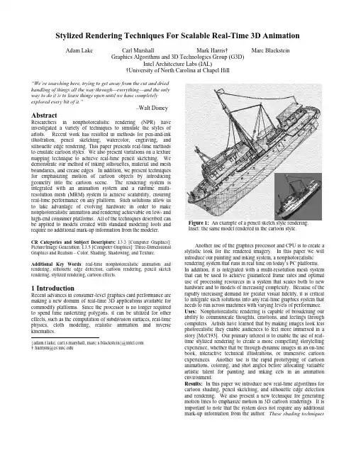
Closing the Smoothness and Uniformity Gap in Area Fill SynthesisYu ChenCS DepartmentUCLALos Angeles,CA90095 yuchen@ Andrew B.KahngCSE and ECEDepartments,UCSDLa Jolla,CA92093abk@Gabriel RobinsCS DepartmentUniversity of VirginiaCharlottesville,VA22903robins@Alexander ZelikovskyCS DepartmentGeorgia State Univ.Atlanta,GA30303alexz@ABSTRACTControl of variability in the back end of the line,and hence in interconnect performance as well,has become extremely difficult with the introduction of new materials such as copper and low-k di-electrics.Uniformity of chemical-mechanical planarization(CMP) requires the addition of areafill geometries into the layout,in order to smoothen the variation of feature densities across the die.Our work addresses the following smoothness gap in the recent litera-ture on areafill synthesis.(1)The veryfirst paper on thefilling problem(Kahng et al.,ISPD98[7])noted that there is potentially a large difference between the optimum window densities infixed dissections vs.when all possible windows in the layout are consid-ered.(2)Despite this observation,allfilling methods since1998 minimize and evaluate density variation only with respect to afixed dissection.This paper gives thefirst evaluation of existingfilling al-gorithms with respect to“gridless”(“floating-window”)mode,ac-cording to both the effective and spatial density models.Our exper-iments indicate surprising advantages of Monte-Carlo and greedy strategies over“optimal”linear programming(LP)based methods. Second,we suggest new,more relevant methods of measuring a local uniformity based on Lipschitz conditions,and empirically demonstrate that Monte-Carlo methods are inherently better than LP with respect to the new criteria.Finally,we propose new LP-basedfilling methods that are directly driven by the new criteria, and show that these methods indeed help close the“smoothness gap”.Categories and Subject DescriptorsB.7.2[Hardware]:IC—Manufacturability;J.6[Computer Ap-plications]:CAD;F.2.2[Analysis of Algorithms]:Problem Com-plexityFigure1:In thefixed-dissection framework,the-by-lay-out is partitioned by(here,)distinct overlapping dis-sections with window size.The layout is partitioned into tiles.Each dark-bordered window consists of tiles.Greedy methods which iterativelyfind the best tile for thenextfilling geometry to be added into the layout.Thesemethods werefirst used in[3]for ILD thickness control,andalso used for shallow-trench isolation(STI)CMP model in[13]);Monte-Carlo(MC)methods,which are similar to greedy meth-ods but insert the nextfilling geometry randomly.Due to itsefficiency and accuracy,these were used for bothflat[3,4]and hierarchical[2]layout density control;andIterated Greedy(IGreedy)and Iterated Monte-Carlo(IMC)methods,which improve the solution quality by iterating theinsertions and deletions of dummyfill features with respectto the density variation([3]).The motivation for our present work is a“smoothness gap”in thefill literature.All existingfilling methods fail to consider the potentially large difference between extremal densities infixed-dissection windows and extremal densities when all possible win-dows are considered.On the other hand,the veryfirst paper in the fill synthesis literature(Kahng et al.,ISPD98[7])already pointedout the gap betweenfixed-dissection and“gridless”analyses,for both tile density and window density.1The potential consequence of the smoothness gap is that thefill result will not satisfy either given upper bounds on post-fill window density,or given bounds on density variation between windows.As post-CMP variation for ox-ide ILD polishing is essentially monotone in window density vari-ation[11],this smoothness gap can compromise manufacturability of the layout,particularly given the small values of in recent de-sign rules.Wefirst address the discretization gap in existing analyses(i.e., evaluations)methods.Previous works compare density control meth-ods only with respect to a givenfixed grid,which underestimates the actual“gridless”density variation,but has been justified on grounds that gridless analysis is impractical.In this paper,we show for thefirst time the viability of gridless orfloating window anal-yses,originally developed for the spatial density model[6],and extend it for the more accurate effective density model[9].Sec-ond,previous research in layout density control concentrated on the global uniformity achieved by minimizing the window density(1) The crucial element of this model is the determination of the effec-tive initial pattern density,.The simplest model foris the local areal feature density,i.e.,the window density is simply equal to the sum:(2) where denotes the original layout area of the tile. This spatial density model is due to[6],which solved the resulting filling problem using linear programming.A more accurate model considers the deformation of the polish-ing pad during the CMP process[5]:effective local densityFigure2:An arbitraryfloating-window always con-tains a shrunk-window of afixed-dissection, and is always covered by a bloated-window of thefixed-dissection.A standardfixed-dissection window is shown with thick border.Afloating window is shown in light gray.The white window is the bloatedfixed-dissection window, and the dark gray window is the shrunkfixed-dissection win-dow.is calculated as the sum of weighted spatial pattern densities within the window,relative to an elliptical weighting function:(3) with experimentally determined constants,,and[12].The discretized effective local pattern density for a window in the fixed-dissection regime(henceforth referred to as effective density) is:(4) where the arguments of the elliptical weighing function are the -and-distances of the tile from the center of the window .2.2Window Density AnalysesThe authors of[6]proposed optimal extremal-density(i.e.,min-imum or maximum window density in the layout)analysis algo-rithms.Their ALG1,with complexity(is the number of rectangles in layout),is proposed as a means of checking the grid-less post-filling density variation.However,with a large number of original and dummyfill features,this algorithm may be infeasible in practice.Another method of[6]overcomes the intractability of optimal extremal-density analysis,based on the following fact(see Fig.2).L EMMA 1.Given afixed-dissection,any arbitrary window will contain some shrunk win-dow of thefixed-dissection,and will be contained in some bloatedwindow of thefixed-dissection.The authors of[6]implemented the above Lemma within a multi-level density analysis algorithm(see Fig.3).Here is used to denote the required user-defined accuracy infinding the maximum window density.The lists TILES and WINDOWS are byproducts of the analysis.Since anyfloating-window is contained in some bloated window,thefilled area in ranges between Max (maximum-windowfilled area found so far)and BloatMax (maximum bloated windowfilled area found so far).The algorithm terminates when the relative gap between Max and BloatMax is at most,and then outputs the middle of the range(Max,BloatMax). We use this algorithm(with accuracy=1.5%)throughout this paper to achieve an accurate,efficient post-filling density analy-Multi-Level Density Analysis Algorithm(1)Make a list ActiveTiles of all-tiles(2)Accuracy,(3)While Accuracy do(a)Find all rectangles in-tiles from ActiveTiles(b)Find area of each window consisting of tiles fromActiveTiles,add such window to the list WINDOWS(c)Max=maximum area of standard window with tilesfrom ActiveTiles(d)BloatMax=maximum area of bloated windowwith tiles from ActiveTiles(e)For each tile from ActiveTiles which do not belong toany bloated window of area more than Max doif Accuracy,then put in TILESremove from ActiveTiles(f)Replace in ActiveTiles each tile with four of its subtiles(g)Accuracy=BloatMax/Max,(4)Move all tiles from ActiveTiles to TILES(5)Output max window density=(Max+BloatMax)Figure3:Multi-level density analysis algorithm.sis.3To handle the effective density model,the multi-level den-sity analysis based on bloated and shrunk windows must be refinedsomewhat.To obtain more accurate results,the multi-level densityanalysis algorithm divides the-dissection into smaller grids,sothat more windows will be considered.With the effective densitymodel,the discretized formulation(effective)shows that effectivelocal pattern density is dependent on the window size and the -dissection.That is,we have to consider the effect on the formu-lation of the further division of layout during post-filling densityanalysis.We assume here that the effective local pattern densityis still calculated with the value of-dissection used in thefillingprocess.The only difference is that the windows phase-shift willbe smaller.For example,in Figure4(a)we calculate the effective density of the window shown in light gray by consideringtiles(also called“cells”)during thefilling process.In Figure4(b)the layout is further partitioned by a factor of.The effective den-sity of the light gray window will be still calculated with the“cells”.Here each“cell”has the same dimension as a tile in thefilling process and consists of smaller tiles.More windows (e.g.,the window with thick border)with smaller phase-shifts will be considered in the more gridded layout.2.3Accurate Analysis of Existing Methods Here we compare the performance of existingfill synthesis meth-ods,using the accurate multilevelfloating-window density analysis. All experiments are performed using part of a metal layer extracted from an industry standard-cell layout4(Table2.3).Benchmark L1 is the M2layer from an8,131-cell design and benchmark L2is the M3layer from a20,577-cell layout.Table2shows that underestimation of the window density varia-tion as well as violation of the maximum window density infixed-(a)(b)Figure4:Post-filling density analysis for the effective density model.(a):afixed-dissection,where each window consists of cells(the same size as tiles);(b):afixed-dissection for post-filling density analysis,where each window consists of smaller tiles and each cell consists of tiles.dissectionfilling can be severe:e.g.,for the LP method applied to the case L2/28/4for the spatial(resp.effective)density model,the density variation is underestimated by210%(resp.264%)and the maximum density is violated by21%(resp.15%).Even for the finest grid(L2/28/16),the LP method may still yield considerable error:11%(resp.23%)in density variation and1.2%(resp.3.2%) in maximum density violation.Note that the LP method cannot easily handle afiner grid since the runtime is proportional to. Our comparisons show that the winning method is IMC and the runner-up is IGreedy.IMC and IGreedy can be run for muchfiner grids since its runtime is proportional to(resp.).Al-though for L2/28/16errors in density variation and the maximum density violation are similar,the iterative methods become consid-erably more accurate.test case L2125,000#rectanglesTable1:Parameters of four industry test cases.Here40units are equivalent to1micron.3.LOCAL DENSITY V ARIATIONThe main objective of layoutfilling is to improve CMP and in-crease yield.Traditionally,layout uniformity has been measured by global spatial or effective density variation over all windows. Such a measure does not take in account that the polishing pad during CMP can change(adjust)the pressure and rotation speed according to the pattern distribution(see[11]).Boning et al.[1] further point out that while the effective density model is excellent for local CMP effect prediction,it fails to take into account global step heights.The influence of density variation between far-apart regions can be reduced by a mechanism of pressure adjustment, which leads to the contact wear model proposed in[1].Within each local region,the areafill can be used to improve the CMP per-formance.Therefore,density variation between two windows in opposite corners of the layout will not cause problems because of the polishing dynamics.According to the integrated contact wear and effective density model,only a significant density variation be-tween neighboring windows will complicate polishing pad control and may cause either dishing or underpolishing.Thus,it is more important to measure density variation between neighboring win-dows.3.1Lipschitz Measures of Smoothness Depending on the CMP process and the polishing pad movement relative to the wafer,we may consider different window“neighbor-hoods”.Below we propose three relevant Lipschitz-like definitions of local density variation which differ only in what windows are considered to be neighbors.Type I:The maximum density variation of every neighbor-ing windows in each row of thefixed-dissection.The intu-ition here is that the polishing pad is moving along window rows and therefore only overlapping windows in the same row define a neighborhood.Type II:The maximum density variation of every cluster of windows which cover one tile.The idea here is that the pol-ishing pad can touch all overlapping windows almost simul-taneously.Type III:The maximum density variation of every cluster of windows which cover one square consisting oftiles.The difference between this and the previous definition is the assumption that the polishing pad is moving slowly;if windows overlap but are still too far from each other,then we can disregard their mutual influence.We compared the behaviors of existingfilling methods with re-spect to these Lipschitz characteristics.The results in Table3show that there is a gap between the traditional Min-Var objective and the new“smoothness”objectives:the solution with the best Min-Var objective value does not always have the best value in terms of“smoothness”objectives.For the spatial(resp.effective)den-sity model,though LP yields the best result for the case L2/28/4 with Min-Var objective withfixed-dissection model,it can not ob-tain the best result with respect to Lipschitz type-I variation.Thus,“smoothness”objectives may be considered separately for thefill-ing process.We also notice that Monte-Carlo methods can achieve better solutions than LP with respect to the“smoothness”objec-tives(note that although LP is“optimal”,it suffers from rounding and discreteness issues when converting the LP solution to an ac-tualfilling solution).3.2Smoothness Objectives for Filling Obviously,all Lipschitz conditions are linear and can be im-plemented as linear programming formulations.We describe four linear programming formulations for the“smoothness”objectives with respect to the spatial density model.(The linear programming formulations for the effective density model are similar.)Thefirst Linear Programming formulation for the Min-Lip-I ob-jective is:Minimize:Subject to:(6)(8) where if,and=1otherwise,andTest case OrgDen FD Multi-Level FD Multi-Level FD Multi-Level FD Multi-Level FD Multi-Level MaxD MaxD MaxD MaxD MaxD MaxDSpatial Density Model.2572.2653.2706.2679.2653.2653 L1/16/16.0417.0896.0915.0705.0773.0705.0758.0705.0755.0705.0753 L2/28/4.0500.0326.1012.0529.0986.0482.0973.0326.0908.0328.0898 .1887.1911.1941.1932.1921.1919Effective Density Model.4161.4244.4251.4286.4245.4251 L1/16/16.0000.2156.2283.2488.2787.1811.2215.1850.2167.1811.2086 .2977.3419.3385.3340.3186.3240 L2/28/16.0000.2417.2987.2417.2946.2617.3161.2302.2916.2533.3097Table2:Multi-level density analysis on results from existingfixed-dissectionfilling methods.Notation:T/W/r:Layout/window size/r-dissection;LP:linear programming method;Greedy:Greedy method;MC:Monte-Carlo method;IGreedy:iterated Greedy method;IMC:iterated Monte-Carlo method;OrgDen:density of original layout;FD:fixed-dissection density analysis; Multi-Level:multi-level density analysis;MaxD:maximum window density;MinD:minimum window density;DenV:density variation.Test case Greedy IGreedyT/W/r LipI LipIII LipI LipIII LipI LipIII LipI LipIII LipI LipIIIL1/16/4.0832.0713.0712.0627.0678.0600.0818.0630.0673.0597.0868.0742.0742.0725.0730 L2/28/4.0414.0841.0412.0893.0289.0852.0333.0755.0286.0766.0642.0713.0658.0619.0631Effective Density Model4.3335.619 4.166 4.254 4.481L1/16/160.8430.8350.978 1.0510.8140.8470.8390.8470.7630.7705.7826.587 5.579 6.317 5.640L2/28/16 1.000 1.159 1.061 1.147 1.115 1.2300.936 1.128 1.112 1.189Table3:Different behaviors of existingfilling methods on”smoothness”objectives.Note:All data for effective density model have been timed by.Notation:LipI:Lipschitz condition I;LipII:Lipschitz condition II;LipIII:Lipschitz condition III.Here,is the given upper bound of the effective tile densities.The constraints(5)imply that features can be added but not deletedfrom any tile.The slack constraints(6)are computed for each tile.The pattern-dependent coefficient denotes the maximumpattern area which can embedded in an empty unit square.If a tile is originally overfilled,then we set.In the LP solution,the values of indicate thefill amount to be insertedin each tile.The constraint(7)says that no window can havedensity greater than than(unless it was initially overfilled).Theconstraints(8)imply that the auxiliary variable is an upper boundon all variation between windows in the same row.The second Linear Programming formulation for the Min-Lip-IIobjective replaces the constraints(8)with the following constraints(9):(10)The constraints(10)ensure that the density variation between any two windows which cover tiles is less than the auxiliary vari-able.Finally,in order to consider the“smoothness”objectives together with the Min-Var objective,we propose another LP formulation with the combined objective which is the linear summation of Min-Var,Lip-I,and Lip-II objectives with specific coefficients.Minimize:Lip-I Constraints(8),Lip-II(9)and Min-Var constraints(11)are added for the combined objective:Test case LipI LP LipIII LPT/W/r DenV Lip2Lip1Lip3DenV Lip2Lip1Lip3DenV Lip2Spatial Density Model.0832.0713.1725.1670.0649.0434.1273.0734.0574.0409.0734.0670.1972.1932.1016.0756.1835.1224.0937.0766.0414.0841.0724.0720.0467.0836.0943.0928.0242.0758.0340.0654.0871.0825.0331.0661.1188.1033.0255.0656L1/16/4.0703.0043.0040.0100.1594.0047.0043.0030.1753.0045L1/16/8.1709.0025.0020.0052.2902.0025.0028.0018.2680.0022L2/28/4.1060.0058.0013.0061.1022.0064.0026.0052.0953.0057L2/28/8.1483.0023.0007.0024.1559.0023.0018.0022.1382.0021The desiredfill area specified for each tile in the LP solution must be rounded to an area that corresponds to an an integer number of dummyfill features.other CMP physical models.We also seek improved methods for optimizingfill synthesis with respect to our new(and possibly other alternative)local uniformity objectives.5.REFERENCES[1]D.Boning,B.Lee,T.Tubawa,and T.Park,“Models forPattern Dependencies:Capturing Effects in Oxide,STI,andCopper CMP”,Semicon/West Tech.Symp.:CMP Tech.forULSI Manuf.,July2001.[2]Y.Chen,A.B.Kahng,G.Robins and A.Zelikovsky,“Hierarchical Dummy Fill for Process Uniformity”,Proc.ASP-DAC,Jan.2001,pp.139-144.[3]Y.Chen,A.B.Kahng,G.Robins and A.Zelikovsky,“Practical Iterated Fill Synthesis for CMP Uniformity”,Proc.Design Automation Conf.,Los Angeles,June2000,pp.671-674.[4]Y.Chen,A.B.Kahng,G.Robins and A.Zelikovsky,“NewMonte-Carlo Algorithms for Layout Density Control”,Proc.ASP-DAC,2000,pp.523-528.[5]R.R.Divecha,B.E.Stine,D.O.Ouma,J.U.Yoon,D.S.Boning,et al.,“Effect of Fine-line Density and Pitch onInterconnect ILD Thickness Variation in Oxide CMPProcess”,Proc.CMP-MIC,1998.[6]A.B.Kahng,G.Robins,A.Singh,H.Wang and A.Zelikovsky,“Filling Algorithms and Analyses for LayoutDensity Control”,IEEE puter-Aided Design18(4)(1999),pp.445-462.[7]A.B.Kahng,G.Robins,A.Singh,H.Wang and A.Zelikovsky,“Filling and Slotting:Analysis and Algorithms”, Proc.ACM/IEEE Intl.Symp.on Physical Design,April1998,pp.95-102.[8]G.Nanz and L.E.Camilletti,“Modeling ofChemical-Mechanical Polishing:A Review”,IEEE Trans.on Semiconductor Manuf.8(4)(1995),pp.382-389.[9]D.Ouma,D.Boning,J.Chung,G.Shinn,L.Olsen,and J.Clark,“An Integrated Characterization and ModelingMethodology for CMP Dielectric Planarization”,Intl.Interconnect Technology Conference,San Francisco,CA,June1998.[10]B.Stine,“A Closed-Form Analytical Model for ILDThickness Variation in CMP Processes”,Proc.CMP-MIC,1997.[11]B.Stine,D.Ouma,R.Divecha,D.Boning and J.Chung,“Rapid Characterization and Modeling of Pattern Dependent Variation in Chemical Mechanical Polishing”,IEEE Trans.Semi.Manuf.,Feb.1998.[12]R.Tian,D.Wong,and R.Boone,“Model-Based DummyFeature Placement for Oxide Chemical Mechanical Polishing Manufacturability”,Proc.Design Automation Conf.,June2000,pp.667-670.[13]R.Tian,X.Tang and D.F.Wong,“Dummy featureplacement for chemical-mechanical polishing uniformity in a shallow trench isolation process”,International Symposium on Physical Design,April2001,pp.118-123.。

Rectilinear Block Placement Using B*-TreesGUANG-MING WUNan-Hua UniversityYUN-CHIH CHANGRealtek Semiconductor Corp.andY AO-WEN CHANGNational T aiwan UniversityDue to the layout complexity in modern VLSI designs,integrated circuit blocks may not be rect-angular.However,literature on general rectilinear block placement is still quite limited.In this article,we present approaches for handling the placement for arbitrarily shaped rectilinear blocks using B*-trees[Chang et al.2000].We derive the feasibility conditions of B*-trees to guide the placement of rectilinear blocks.Experimental results show that our algorithm achieves optimal or near-optimal block placement for benchmarks with various shaped blocks.Categories and Subject Descriptors:B7.2[Integrated Circuits]:Design Aids—placement and routing;J.6[Computer Applications]:Computer-Aided EngineeringGeneral Terms:Algorithms,Design,Experimentation,Measurement,PerformanceAdditional Key Words and Phrases:Computer-aided design of VLSI,floorplanning,layout, placement1.INTRODUCTIONDue to the growth in design complexity,circuit size is getting larger.To cope with the increasing design complexity,hierarchical design and IP modules are widely used.This trend makes blockfloorplanning/placement much more critical to the quality of a design.Floorplanning is often studied based on twofloorplan structures,the slicing structure[Otten1982;Wong and Liu1986]and the nonslicing structure[Chang The work of G.-M.Wu was partially supported by the National Science Council of Taiwan ROC under Grant No.NSC-91-2215-E-343-001.The work of Y.-W.Chang was partially supported by the National Science Council of Taiwan ROC under Grant No.NSC-91-2215-E-002-038.Authors’addresses:G.-M.Wu,Department of Information Management,Nan-Hua University, Chiayi,Taiwan;email:*************.edu.tw;Y.-C.Chang,Realtek Semiconductor Corp.,No.2, Industry E.Rd.IX,Science-Based Industrial Park,Hsinchu,Taiwan;Y.-W.Chang,Graduate In-stitute of Electronics Engineering and Department of Electrical Engineering,National Taiwan University,Rm.548,Electrical Engineering Building#1,Taipei106,Taiwan;email:ywchang@ .tw.Permission to make digital/hard copy of part or all of this work for personal or classroom use is granted without fee provided that the copies are not made or distributed for profit or commercial advantage,the copyright notice,the title of the publication,and its date appear,and notice is given that copying is by permission of the ACM,Inc.To copy otherwise,to republish,to post on servers, or to redistribute to lists,requires prior specific permission and/or a fee.C 2003ACM1084-4309/03/0400-0188$5.00ACM Transactions on Design Automation of Electronic Systems,Vol.8,No.2,April2003,Pages188–202.Rectilinear Block Placement Using B*-T rees•189 et al.2000;Guo et al.1999;Murata et al.1997;Nakatake et al.1996;Wang and Wong1990].A slicing structure can be represented by a binary tree whose leaves denote modules,and internal nodes specify horizontal or vertical cut lines.Wong and Liu[1986]proposed an algorithm for slicingfloorplan design. They presented a normalized Polish expression to represent a slicing structure, enabling the speedup of the search procedure.However,this representation can-not handle nonslicingfloorplans.Recently,researchers have proposed several representations for nonslicingfloorplans,such as the sequence pair[Murata et al.1997],bounded slicing grid(BSG)[Nakatake et al.1996],O-tree[Guo et al.1999],and B*-tree[Chang et al.2000].In modern VLSI design,the blocks may not be rectangular.Most existing floorplanning/placement algorithms,however,only deal with rectangles and cannot apply to arbitrarily shaped rectilinear block placement directly.New approaches that can handle arbitrarily shaped blocks are essential to optimize resource(e.g.,area)utilization.Preas and van Cleemput[1979]proposed a graph model for the topological re-lationships among rectangular and arbitrarily shaped rectilinear blocks.Wong and Liu[1987]extended the Polish expression to represent slicingfloorplans with rectangular and L-shaped blocks.Lee[1993]extended the zone refinement technique to rectilinear blocks.A bounded2-D contour searching algorithm was proposed tofind the best position for a block.Kang and Dai[1997]proposed a BSG-based method to solve the packing of rectangular,L-shaped,T-shaped,and soft blocks.The algorithm combined simulated annealing and a genetic algorithm for general nonslicingfloorplans.Xu et al.[1998]presented an approach extending the sequence-pair approach for rectangular block placement to arbitrarily sized and shaped rectilinear blocks.The properties of L-shaped blocks were examinedfirst,and then arbi-trarily shaped rectilinear blocks were decomposed into a set of L-shaped blocks.Kang and Dai[1998]proposed a method based on the sequence-pair structure for rectilinear block placement.Three necessary and sufficient conditions for a sequence pair to be feasible were derived.A stochastic search was applied on the optimization of convex blockfloorplanning.Chang et al.[2000]recently proposed the B*-tree representation for nonslic-ingfloorplans,which is based on block compaction and ordered binary trees. Inheriting from the nice properties of ordered binary trees,B*-trees are very easy to implement and require only constant time for tree search and insertion, and linear time for deletion.Unlike the O-tree representations,in particular, no extra encoding of the tree itself is needed for a B*-tree,and cost evalua-tion can be performed directly on a B*-tree.Besides,the ordered property of a B*-tree makes the incremental cost evaluation of its corresponding placement possible.Furthermore,given a B*-tree,it takes only linear time to construct the placement,and vice versa.All these nice properties make the B*-trees an efficient andflexible representation for nonslicingfloorplans.In this article,we apply the B*-tree to handle the placement of arbitrarily shaped rectilinear blocks.First,we explore the properties of L-shaped blocks and then extend the properties to general rectilinear blocks.The feasibility con-ditions are then used to guide the placement of rectilinear blocks.We construct a ACM Transactions on Design Automation of Electronic Systems,Vol.8,No.2,April2003.190•G.M.Wu et al.Top profile sequence = (4, [5, 7], [7, 4], [6, 1], [8, 4])Fig.1.The top profile sequence consists of the length of the base,followed by a sequence of two-tuples that is composed of the lengths of the succeeding horizontal segments and their relative heights to the base.set of benchmarks with rectangular and L-shaped(and T-shaped)blocks and ap-ply simulated annealing as a vehicle to test the effectiveness of our approaches. Experiment results show that our approaches lead to placements with optimal or near-optimal area utilization.The remainder of this article is organized as follows.Section2formulates the rectilinear block placement problem.Section3introduces the B*-tree repre-sentation.Section4describes the method for the L-shaped blocks in a B*-tree. Section5describes our algorithm.Section6extends the algorithm to arbitrar-ily rectilinear blocks.Experimental results are reported in Section7.Finally, we give conclusions in Section8.2.FORMULATIONLet B={b1,b2,...,b n}denote a set of rectilinear blocks.A block is notflex-ible in its shape but free to rotate andflip.A packing of a set of blocks is a nonoverlapping placement of the blocks.A rectilinear block can be represented by four profile sequences,namely,the top profile sequence,the bottom profile sequence,the left profile sequence,and the right profile sequence,specifying the profiles viewed from the top side,the bottom side,the left side,and the right side of the block,respectively.The top (bottom)profile sequence of a rectilinear block uses the leftmost horizontal segment on the top(bottom)boundary of the block as a base and records the length of the succeeding horizontal segments on the top(bottom)boundary and the relative height.Specifically,the top profile sequence consists of the length of the base,followed by a sequence of two-tuples composed of the lengths of the succeeding horizontal segments and their relative heights to the base(could be negative).For example,Figure1shows a rectilinear block with the top profile sequence(4,[5,7],[7,4],[6,−1],[8,4]).The base of the sequence is segment a which has a length of4units.The second horizontal segment is c which has a length of5units and is7units higher than the base a.Similarly,the third horizontal segment is e which has a length of7units and is4units higher ACM Transactions on Design Automation of Electronic Systems,Vol.8,No.2,April2003.Rectilinear Block Placement Using B*-T rees•191(a)01b b b b b b b b (0, 0)x y 23456b 780123678(b)n 4n n 5n n n n n n Fig.2.An admissible placement and its corresponding B*-tree.than the base a ,and so on.The other three profile sequences are similarly defined.Definition 1.A rectilinear block placement is feasible if and only if no two blocks overlap each other,and all profile sequences remain unchanged after placement (i.e.,all blocks keep their original shapes).The goal of the rectilinear placement problem is to optimize a given cost metric (such as area,wirelength,etc.)induced by the assignment of b i s.(By area here,we mean the final enclosing rectangle of B .)3.OVERVIEW OF THE B*-TREE REPRESENTATIONGiven an admissible placement P ,we can represent it by a unique (horizontal)B*-tree T [Chang et al.2000].(See Figure 2(b)for the B*-tree representing the placement shown in Figure 2(a).)A B*-tree is an ordered binary tree whose root corresponds to the module in the bottom-left corner.Similar to the depth-first search (DFS)procedure,we construct the B*-tree T for an admissible placement P in a recursive fashion.Starting from the root,we first recursively construct the left subtree and then the right subtree.Let R i denote the set of modules located on the right-hand side and adjacent to b i .The left child of the node n i corresponds to the lowest module in R i that is unvisited.The right child of n i represents the first module located above and visible from b i ,with its x -coordinate equal to that of b i (and its y -coordinate less than or equal to that of the top boundary of the module on the left-hand side and adjacent to b i ,if any ,to consider the special placement).As shown in Figure 2,we make n 0the root of T since b 0is in the bottom-left corner.Constructing the left subtree of n 0recursively ,we make n 4the left child of n 0.Since the left child of n 4does not exist,we then construct the right subtree of n 4(which is rooted by n 5).The construction is recursively performed in the DFS order.After completing the left subtree of n 0,the same procedure applies to the right subtree of n 0.Figure 2(b)illustrates the resulting B*-tree for the placement shown in Figure 2(a).The construction takes only linear time.ACM Transactions on Design Automation of Electronic Systems,Vol.8,No.2,April 2003.192•G.M.Wu et al.old contournew contourFig.3.A contour and its update:when adding a new block to the placement,we search the contour from left to right and update it with the top boundary of the new block.The B*-tree keeps the geometric relationship between two modules as fol-lows.If node n j is the left child of node n i,module b j must be located on theright-hand side and adjacent to module b i in the admissible placement;thatis,x j=x i+w i.Besides,if node n j is the right child of n i,module b j must be located above and visible from module b i,with the x-coordinate of b j equalto that of b i;that is,x j=x i.Also,since the root of T represents the bottom-left module,the x-and y-coordinates of the module associated with the root (x root,y root)=(0,0).A contour structure(see Figure3),which was originally proposed in Guo et al.[1999],can be used to reduce the run-time offinding the y-coordinate of a newlyinserted block.The contour structure is a doubly linked list of blocks,whichdescribes the contour line in the current compaction direction.Without thecontour structure,the run-time for placing a new block is linear to the numberof blocks.By maintaining the contour structure,however,the y-coordinate ofa block can be computed in O(1)time.Figure3illustrates how to update thecontour when we add a new block to the placement.4.L-SHAPED BLOCKSIn this section,we apply the B*-tree approach tofind a feasible placement withL-shaped blocks.Let b L denote an L-shaped block.b L can be partitioned intotwo rectangular subblocks by slicing b L along its middle vertical boundary.Asshown in Figure4(a),b1and b2are the subblocks of b L,and we say b1,b2∈b L.After partitioning and placement,the rectilinear block b L might not conformto its top profile sequence,as illustrated in Figure5.Figure5(a)shows a B*-tree and its corresponding placement.We can pull subblock b2up to align withthe subblock b1,so that the block b L can maintain its top profile sequence with-out changing the overall topology of the blocks.Conversely,there might not beenough space to do so;see Figure5(b)for such an example.It is obvious thata feasible placement can be generated from the B*-tree shown in Figure5(a)with a local adjustment,but it is impossible for the case shown in Figure5(b).Therefore,if we represent an L-shaped block by two subblocks,we must guar-antee that the two subblocks abut.To ensure that the left subblock b1and the ACM Transactions on Design Automation of Electronic Systems,Vol.8,No.2,April2003.Rectilinear Block Placement Using B*-T rees •193(a)(b)(c)(d)(e)(f)(g)(h)b1b2b2b2b2b2b1b1b1b1b1b1b1b2b2b2Fig.4.Eight situationsof an L-shaped block.Each is partitionedinto two parts by slicing it along the middle vertical boundary .(b)Fig.5.Placing the L-shaped block shown in Figure 4(a)by two subblocks:(a)a feasible placement;(b)an infeasible placement.right subblock b 2of an L-shaped block b L abut,we impose the following location constraint (LC for short)for b 1and b 2.LC :Keep b 2as b 1’s left child in the B*-tree.The LC relation ensures that the x -coordinate of the left boundary of b 2is equal to that of the right boundary of b 1.For example,the two sets of subblocks b 1,b 2and b 3,b 4shown in Figure 6(a)do not abut whereas those shown in Figure 6(b)ACM Transactions on Design Automation of Electronic Systems,Vol.8,No.2,April 2003.194•G.M.Wu et al.Fig.6.Suppose that b1,b2and b3,b4are two sets of subblocks corresponding to two L-shaped blocks(a)a placement in which b1,b2and b3,b4do not abut.Their corresponding nodes in the B*-tree may not be related;(b)another placement in which b1,b2and b3,b4abut.Their corresponding nodes in the B*-tree keep the LC relation between b1and b2(as well as b3and b4).do.In Figure6(b),the subblocks b3and b4are placed at the right locations and the subblocks b1and b2are not since the y-coordinates of b1and b2are not equal.We say b1and b2are misaligned.In the following,we adopt the contour data structure to solve the misalign-ment problem.When transforming a B*-tree to its corresponding placement, we update the contour to maintain its top profile sequence as follows.Assume that b1and b2are the respective left and right subblocks of an L-shaped block b L,and they are misaligned.When processing b2,b1must have been placed.We can classify the misalignment into categories and adjust them as follows. (1)Basin:The contour is lower than the top profile sequence at the positionof the current subblock b2.(See Figure7(a).)In this case,we pull b2up to conform to the top profile sequence of the L-shaped block b L.It should be noted that this operation will not pull other blocks up due to the DFS packing order induced by the B*-tree.(2)Plateau:The contour is higher than the top profile sequence at the positionof the current subblock b2.(See Figure7(b).)In this case,we pull b1up to conform to the top profile sequence of b L.(Note that b2cannot be moved down because the compaction operation makes b2be placed right above another block.)It is clear that each of the adjustments can be performed in constant time with the contour data structure.In the following,we discuss the rotation andflip operations of an L-shaped block.For each L-shaped block b i,there are eight orientations by rotation and ACM Transactions on Design Automation of Electronic Systems,Vol.8,No.2,April2003.Rectilinear Block Placement Using B*-T rees•195(a)(b)Fig.7.Placing two subblocks b1and b2of an L-shaped block:(a)if the contour is lower than the top profile sequence at b2,then we pull b2up to meet the top profile sequence;(b)if the contour is higher than the top profile sequence at b2,then we pull b1up to meet the top profile sequence.flip,as shown in Figure4.To preserve the LC relation and keep it in the B*-tree, we repartition b i into two subblocks after it is rotated orflipped and keep the LC relation between them.Figure4shows the subblocks after repartitioning. As shown in thefigure,an L-shaped block is always partitioned by slicing it along the middle vertical boundary.After repartitioning,we should update the top profile sequence for the block.5.FLOORPLAN ALGORITHMOur rectilinearfloorplan design algorithm is based on the simulated annealing method[Kirkpatrick et al.1983;Sechen and Sangiovanni1985]and the B*-tree described in Section3.We perturb a B*-tree(a feasible solution)to another B*-tree by using the following four operations.Op1:Rotate a block.Op2:Flip a block.Op3:Move a block to another place.Op4:Swap two blocks.The Op1and Op2operations have been described in Section4.The Op3opera-tion deletes and inserts a block into a B*-tree.If the deleted node is associated with a rectangular block,we simply delete the node from the B*-tree.Other-wise,there will be two nodes associated with an L-shaped block,and we must delete the two nodes from the B*-tree and insert them in other places.Note that the LC relations must hold.Both of the Op3and Op4operations need to apply the Insert(n i)and Delete(n i)operations,where Insert(n i)(Delete(n i))is the operation for inserting(deleting)a node n i to(from)a B*-tree.The B*-tree must remain a binary tree after deletion or insertion.We detail the deletion and insertion operations in the following.5.1DeletionThe deletion can be categorized into these cases:—Case1:A leaf node;—Case2:A node with one child;—Case3:A node with two children.ACM Transactions on Design Automation of Electronic Systems,Vol.8,No.2,April2003.196•G.M.Wu et al.Fig.8.Deletion:(a)deleting a leaf node;(b)deleting a node with only one child;(c)deleting a node with two children.In Case1,we can just delete the target leaf node directly,and the tree will still be a B*-tree.As shown in Figure8(a),to delete the node n7from the B*-tree of Figure2,we set the left childfield of its parent n6to be NULL and free the node n7.In Case2,we remove the target node and then place the single child at the position of the removed node.For example,after deleting the node n4from the B*-tree of Figure2,we move n5to the original position of n4and obtain the tree shown in Figure8(b).This tree update can be performed in O(1)time. Note that the relative positions of the blocks might be changed after the op-eration,and thus we might need to reconstruct a corresponding placement for further processing.In Case3,when deleting a target node n t with two children,we replace n t by either its right child or left child n c.Then we move a child of n c to the original position of n c.The process proceeds until the corresponding leaf node is handled.For instance,suppose that we delete the node n0from the B*-tree of Figure2.We can use the right child n1to replace it,and then use n3to replace n1.(The resulting tree is shown in Figure8(c).)It is obvious that such a deletion operation requires O(h)time,where h is the height of the B*-tree.Again the ACM Transactions on Design Automation of Electronic Systems,Vol.8,No.2,April2003.Rectilinear Block Placement Using B*-T rees•197Fig.9.The inseparable,internal,and external positions of a B*-tree.(Assume that n1and n2 are associated with the same L-shaped block.)A node can be inserted at either an internal or an external position.relative positions of the blocks might be changed after the operation,and thus we might need to reconstruct a corresponding placement for further processing.Note that if the deleted node n i is a subblock of an L-shaped b L,we should also delete the other subblock of b L.5.2InsertionWhen adding a block to a placement,we may place the block around a certain block,but not between two subblocks that belong to an L-shaped block.For a B*-tree,we define three types of positions as follows.(See Figure9for an illustration.)—Inseparable position:A position between two nodes associated with the two subblocks of an L-shaped block.—Internal position:A position between two nodes in a B*-tree,but not an inseparable one.—External position:A position pointed to by a NULL pointer.Only internal and external positions can be used for inserting a new node.For a rectangular block,we can insert it into an internal or an external position directly.For any L-shaped block b L consisting of two subblocks b1and b2,with b1on the left-hand side of b2,the two subblocks must be inserted into a B*-tree simultaneously,and b2must be the left child of b1(according to the LC relation).In the following,we discuss three cases of inserting an L-shaped block into an internal position.As shown in Figure10,if we insert two nodes b1and b2of an L-shaped block into an internal position between nodes b i and b j,with b j being a child of b i,b j can be placed at the position that is the left child of b2, the right child of b2,or the right child of b1.ACM Transactions on Design Automation of Electronic Systems,Vol.8,No.2,April2003.198•G.M.Wu et al.(a)(d)Fig.10.Three cases of inserting an L-shaped block to an internal position.b1b2b3b4b5b6b7(a)b1b2b3b4b5b6(b)Fig.11.(a)Partition a convex block along every vertical boundary from left to right;(b)repartition the block of (a)after it rotates.6.EXTENSION TO GENERAL RECTILINEAR BLOCKSIn this section,we extend the techniques described in previous sections to han-dle general rectilinear blocks.In general,a rectilinear block can be partitioned into a set of rectangular subblocks.Let b i denote an arbitrarily shaped rectilin-ear block.b i can be partitioned into a set of rectangular subblocks by slicing b i from left to right along every vertical boundary of b i ,as shown in Figure 11(a).After perturbing the Op1and Op2operations,we repartition a recti-linear block when it is rotated or flipped.Figure 11(b)shows the block of ACM Transactions on Design Automation of Electronic Systems,Vol.8,No.2,April 2003.Rectilinear Block Placement Using B*-T rees•199Fig.12.Filling approximation for a rectilinear block.Figure11(a)after rotating90◦clockwise;there are six subblocks in it after the repartition.There are two types of rectilinear blocks:convex and concave.A rectilinear block is convex if any two points within the block can be connected by a shortest Manhattan path that also lies within the block;the block is concave,otherwise. Figures11and12show two convex and a concave block,respectively.A convex block b C can be partitioned into a set of subblocks b1,b2,...,b n ordered from left to right.Considering the LC relation,we keep the subblock b i+1as b i’s left child in the B*-tree to ensure that they are placed side by side along the x-direction, where1≤i≤n−1.To ensure that b1,b2,...,b n are not misaligned,we modify the processing for Basin and Plateau as follows.—Basin:The contour is lower than the top profile sequence at the position of a subblock.We pull the subblock up to conform to the top profile sequence.—Plateau:The top boundary of a subblock b i(1≤i≤n)in the contour is higher than the top profile sequence at the position of b i.Assume that b i has the largest top boundary.We pull all subblocks,except b i,up to conform to the top profile sequence.Moreover,all subblocks must be deleted(or inserted)together for the OP3and OP4operations.For a concave block,there might be empty space between two subblocks.As shown in Figure12,the subblock b1is placed above the subblock b2,which cannot be characterized by an LC relation in the B*-tree.Nevertheless,we can fill the concave holes of a concave block and make it a convex block.We call this operation afilling approximation for the rectilinear block.For any concave block,we treat it as a convex block after applying appropriatefilling.7.EXPERIMENTAL RESULTSWe implemented our algorithm in the C++programming language on a 450MHz SUN Ultra Sparc-I workstation with1Gb memory.Since the bench-marks in previous work are artificial cases and unavailable to us,we generate some general benchmarks for experiments in this article.Our test cases were generated by cutting a rectangle into a set of blocks.Therefore,the optimum area is given by the original block.As shown in Table I,Columns2through4list the numbers of rectangular, L-shaped,and T-shaped blocks.RL10,RL20,and RL30consist of only ACM Transactions on Design Automation of Electronic Systems,Vol.8,No.2,April2003.200•G.M.Wu et al.Table I.Experimental Results #Rectangular #L-Shaped #T-Shaped OptimumResulting Dead Run-time Circuits Blocks Blocks Blocks AreaArea Space (%)(sec)RL105501001000.008(10×10)(10×10)RL2010100400408 2.00307(20×20)(15×27)RL3015150900936 4.001636(30×30)(29×32)RLT10433100102 2.0041(10×10)(6×17)RLT20776400414 3.501096(20×20)(18×23)RLT30101010900945 5.003007(30×30)(27×35)(a)12345678910(b)11098546372Fig.13.Placement for RL10:5rectangular and 5L-shaped blocks:(a)the optimum placement (10×10);(b)the resulting placement (10×10).rectangular and L-shaped blocks.There are 5rectangular and 5L-shaped blocks in RL10,10rectangular and 10L-shaped blocks in RL20,and 15rectan-gular and 15L-shaped blocks in RL30,respectively .RLT10,RLT20,and RLT30consist of not only rectangular and L-shaped blocks,but also T-shaped ones.RLT10is composed of 4rectangular,3L-shaped,and 3T-shaped blocks;RLT20is composed of 7rectangular,7L-shaped,and 6T-shaped blocks;and RLT30is composed of 10rectangular,10L-shaped,and 10T-shaped blocks.The original area of each test case is shown in Column 5.Columns 6and 7list the result-ing area and the dead space (%).The results show that our algorithm obtains the optimum area for RL10and near optimum areas for RL20,RL30,RLT10,RLT20,and RLT30with areas only 2.00,4.00,2.00,3.50,and 5.00%away from the optima,respectively .The run-times for achieving the results ranged from about 8seconds to 50minutes (see Column 8).Figures 13and 14show the optimum and the resulting placement for RL10and RLT30,respectively .ACM Transactions on Design Automation of Electronic Systems,Vol.8,No.2,April 2003.Rectilinear Block Placement Using B*-T rees •201(a)123456789101112131415161718192021222324252627282930123456789101113121920142115161718263029252824232722(b)Fig.14.Placement for RLT30:10rectangular,10L-shaped,and 10T-shaped blocks:(a)the opti-mum placement (30×30);(b)the resulting placement (27×35).8.CONCLUSIONSIn this article,we have extended the B*-tree approach introduced in Chang et al.[2000]to handle the placement of arbitrarily shaped rectilinear blocks.We partitioned a rectilinear block into a set of rectangular subblocks,each indi-vidually represented by a node in the B*-tree.The LC relations and the basin and plateau operations were used to ensure that each block kept its original shape.The experiment results have shown that our approach is very effective in area utilization.REFERENCESC HANG ,Y.-C.,C HANG ,Y.-W .,W U ,G.-M.,AND W U ,S.-W .2000.B*-Trees:A new representation for non-slicing floorplans.In Proceedings of the ACM/IEEE Design Automation Conference ,(Los Angeles,June),458–463.G UO ,P .-N.,C HENG ,C.-K.,AND Y OSHIMURA ,T .1999.An O-tree representation of non-slicing floor-plan and its applications.In Proceedings of the ACM/IEEE Design Automation Conference (California,June),268–273.P APADIMITRIOU ,C.AND S TEIGLITZ ,binatorial Optimization:Algorithms and Complex-ity .Prentice-Hall Inc.,Englewood Cliffs,NJ.K ANG ,M.Z.AND D AI ,W .1997.General floorplanning with L-shaped,T-shaped and soft blocks based on bounded slicing grid structure.In Proceedings of the ACM/IEEE Asia and South Pacific Design Automation Conference (Chiba,Japan,January 28–31),265–270.K ANG ,M.Z.AND D AI ,W .1998.Arbitrary rectilinear block packing based on sequence pair.In Proceedings of the ACM/IEEE International Conference on Computer-Aided Design (San Jose,CA,November 8–12),259–266.K IRKPATRICK ,S.,G ELATT ,C.D.,AND V ECCHI ,M.P .1983.Optimization by simulated annealing.Science 220,4598,671–680.L EE ,T .C.1993.A bounded 2D contour searching algorithm for floorplan design with arbitrar-ily shaped rectilinear and soft modules.In Proceedings of the ACM/IEEE Design Automation Conference (California,June),525–530.ACM Transactions on Design Automation of Electronic Systems,Vol.8,No.2,April 2003.。

A modified version of this technical report will appear in ACM Computing Surveys,September2009. Anomaly Detection:A SurveyVARUN CHANDOLAUniversity of MinnesotaARINDAM BANERJEEUniversity of MinnesotaandVIPIN KUMARUniversity of MinnesotaAnomaly detection is an important problem that has been researched within diverse research areas and application domains.Many anomaly detection techniques have been specifically developed for certain application domains,while others are more generic.This survey tries to provide a structured and comprehensive overview of the research on anomaly detection.We have grouped existing techniques into different categories based on the underlying approach adopted by each technique.For each category we have identified key assumptions,which are used by the techniques to differentiate between normal and anomalous behavior.When applying a given technique to a particular domain,these assumptions can be used as guidelines to assess the effectiveness of the technique in that domain.For each category,we provide a basic anomaly detection technique,and then show how the different existing techniques in that category are variants of the basic tech-nique.This template provides an easier and succinct understanding of the techniques belonging to each category.Further,for each category,we identify the advantages and disadvantages of the techniques in that category.We also provide a discussion on the computational complexity of the techniques since it is an important issue in real application domains.We hope that this survey will provide a better understanding of the different directions in which research has been done on this topic,and how techniques developed in one area can be applied in domains for which they were not intended to begin with.Categories and Subject Descriptors:H.2.8[Database Management]:Database Applications—Data MiningGeneral Terms:AlgorithmsAdditional Key Words and Phrases:Anomaly Detection,Outlier Detection1.INTRODUCTIONAnomaly detection refers to the problem offinding patterns in data that do not conform to expected behavior.These non-conforming patterns are often referred to as anomalies,outliers,discordant observations,exceptions,aberrations,surprises, peculiarities or contaminants in different application domains.Of these,anomalies and outliers are two terms used most commonly in the context of anomaly detection; sometimes interchangeably.Anomaly detectionfinds extensive use in a wide variety of applications such as fraud detection for credit cards,insurance or health care, intrusion detection for cyber-security,fault detection in safety critical systems,and military surveillance for enemy activities.The importance of anomaly detection is due to the fact that anomalies in data translate to significant(and often critical)actionable information in a wide variety of application domains.For example,an anomalous traffic pattern in a computerTo Appear in ACM Computing Surveys,092009,Pages1–72.2·Chandola,Banerjee and Kumarnetwork could mean that a hacked computer is sending out sensitive data to an unauthorized destination[Kumar2005].An anomalous MRI image may indicate presence of malignant tumors[Spence et al.2001].Anomalies in credit card trans-action data could indicate credit card or identity theft[Aleskerov et al.1997]or anomalous readings from a space craft sensor could signify a fault in some compo-nent of the space craft[Fujimaki et al.2005].Detecting outliers or anomalies in data has been studied in the statistics commu-nity as early as the19th century[Edgeworth1887].Over time,a variety of anomaly detection techniques have been developed in several research communities.Many of these techniques have been specifically developed for certain application domains, while others are more generic.This survey tries to provide a structured and comprehensive overview of the research on anomaly detection.We hope that it facilitates a better understanding of the different directions in which research has been done on this topic,and how techniques developed in one area can be applied in domains for which they were not intended to begin with.1.1What are anomalies?Anomalies are patterns in data that do not conform to a well defined notion of normal behavior.Figure1illustrates anomalies in a simple2-dimensional data set. The data has two normal regions,N1and N2,since most observations lie in these two regions.Points that are sufficiently far away from the regions,e.g.,points o1 and o2,and points in region O3,are anomalies.Fig.1.A simple example of anomalies in a2-dimensional data set. Anomalies might be induced in the data for a variety of reasons,such as malicious activity,e.g.,credit card fraud,cyber-intrusion,terrorist activity or breakdown of a system,but all of the reasons have a common characteristic that they are interesting to the analyst.The“interestingness”or real life relevance of anomalies is a key feature of anomaly detection.Anomaly detection is related to,but distinct from noise removal[Teng et al. 1990]and noise accommodation[Rousseeuw and Leroy1987],both of which deal To Appear in ACM Computing Surveys,092009.Anomaly Detection:A Survey·3 with unwanted noise in the data.Noise can be defined as a phenomenon in data which is not of interest to the analyst,but acts as a hindrance to data analysis. Noise removal is driven by the need to remove the unwanted objects before any data analysis is performed on the data.Noise accommodation refers to immunizing a statistical model estimation against anomalous observations[Huber1974]. Another topic related to anomaly detection is novelty detection[Markou and Singh2003a;2003b;Saunders and Gero2000]which aims at detecting previously unobserved(emergent,novel)patterns in the data,e.g.,a new topic of discussion in a news group.The distinction between novel patterns and anomalies is that the novel patterns are typically incorporated into the normal model after being detected.It should be noted that solutions for above mentioned related problems are often used for anomaly detection and vice-versa,and hence are discussed in this review as well.1.2ChallengesAt an abstract level,an anomaly is defined as a pattern that does not conform to expected normal behavior.A straightforward anomaly detection approach,there-fore,is to define a region representing normal behavior and declare any observation in the data which does not belong to this normal region as an anomaly.But several factors make this apparently simple approach very challenging:—Defining a normal region which encompasses every possible normal behavior is very difficult.In addition,the boundary between normal and anomalous behavior is often not precise.Thus an anomalous observation which lies close to the boundary can actually be normal,and vice-versa.—When anomalies are the result of malicious actions,the malicious adversaries often adapt themselves to make the anomalous observations appear like normal, thereby making the task of defining normal behavior more difficult.—In many domains normal behavior keeps evolving and a current notion of normal behavior might not be sufficiently representative in the future.—The exact notion of an anomaly is different for different application domains.For example,in the medical domain a small deviation from normal(e.g.,fluctuations in body temperature)might be an anomaly,while similar deviation in the stock market domain(e.g.,fluctuations in the value of a stock)might be considered as normal.Thus applying a technique developed in one domain to another is not straightforward.—Availability of labeled data for training/validation of models used by anomaly detection techniques is usually a major issue.—Often the data contains noise which tends to be similar to the actual anomalies and hence is difficult to distinguish and remove.Due to the above challenges,the anomaly detection problem,in its most general form,is not easy to solve.In fact,most of the existing anomaly detection techniques solve a specific formulation of the problem.The formulation is induced by various factors such as nature of the data,availability of labeled data,type of anomalies to be detected,etc.Often,these factors are determined by the application domain inTo Appear in ACM Computing Surveys,092009.4·Chandola,Banerjee and Kumarwhich the anomalies need to be detected.Researchers have adopted concepts from diverse disciplines such as statistics ,machine learning ,data mining ,information theory ,spectral theory ,and have applied them to specific problem formulations.Figure 2shows the above mentioned key components associated with any anomaly detection technique.Anomaly DetectionTechniqueApplication DomainsMedical InformaticsIntrusion Detection...Fault/Damage DetectionFraud DetectionResearch AreasInformation TheoryMachine LearningSpectral TheoryStatisticsData Mining...Problem CharacteristicsLabels Anomaly Type Nature of Data OutputFig.2.Key components associated with an anomaly detection technique.1.3Related WorkAnomaly detection has been the topic of a number of surveys and review articles,as well as books.Hodge and Austin [2004]provide an extensive survey of anomaly detection techniques developed in machine learning and statistical domains.A broad review of anomaly detection techniques for numeric as well as symbolic data is presented by Agyemang et al.[2006].An extensive review of novelty detection techniques using neural networks and statistical approaches has been presented in Markou and Singh [2003a]and Markou and Singh [2003b],respectively.Patcha and Park [2007]and Snyder [2001]present a survey of anomaly detection techniques To Appear in ACM Computing Surveys,092009.Anomaly Detection:A Survey·5 used specifically for cyber-intrusion detection.A substantial amount of research on outlier detection has been done in statistics and has been reviewed in several books [Rousseeuw and Leroy1987;Barnett and Lewis1994;Hawkins1980]as well as other survey articles[Beckman and Cook1983;Bakar et al.2006].Table I shows the set of techniques and application domains covered by our survey and the various related survey articles mentioned above.12345678TechniquesClassification Based√√√√√Clustering Based√√√√Nearest Neighbor Based√√√√√Statistical√√√√√√√Information Theoretic√Spectral√ApplicationsCyber-Intrusion Detection√√Fraud Detection√Medical Anomaly Detection√Industrial Damage Detection√Image Processing√Textual Anomaly Detection√Sensor Networks√Table parison of our survey to other related survey articles.1-Our survey2-Hodge and Austin[2004],3-Agyemang et al.[2006],4-Markou and Singh[2003a],5-Markou and Singh [2003b],6-Patcha and Park[2007],7-Beckman and Cook[1983],8-Bakar et al[2006]1.4Our ContributionsThis survey is an attempt to provide a structured and a broad overview of extensive research on anomaly detection techniques spanning multiple research areas and application domains.Most of the existing surveys on anomaly detection either focus on a particular application domain or on a single research area.[Agyemang et al.2006]and[Hodge and Austin2004]are two related works that group anomaly detection into multiple categories and discuss techniques under each category.This survey builds upon these two works by significantly expanding the discussion in several directions. We add two more categories of anomaly detection techniques,viz.,information theoretic and spectral techniques,to the four categories discussed in[Agyemang et al.2006]and[Hodge and Austin2004].For each of the six categories,we not only discuss the techniques,but also identify unique assumptions regarding the nature of anomalies made by the techniques in that category.These assumptions are critical for determining when the techniques in that category would be able to detect anomalies,and when they would fail.For each category,we provide a basic anomaly detection technique,and then show how the different existing techniques in that category are variants of the basic technique.This template provides an easier and succinct understanding of the techniques belonging to each category.Further, for each category we identify the advantages and disadvantages of the techniques in that category.We also provide a discussion on the computational complexity of the techniques since it is an important issue in real application domains.To Appear in ACM Computing Surveys,092009.6·Chandola,Banerjee and KumarWhile some of the existing surveys mention the different applications of anomaly detection,we provide a detailed discussion of the application domains where anomaly detection techniques have been used.For each domain we discuss the notion of an anomaly,the different aspects of the anomaly detection problem,and the challenges faced by the anomaly detection techniques.We also provide a list of techniques that have been applied in each application domain.The existing surveys discuss anomaly detection techniques that detect the sim-plest form of anomalies.We distinguish the simple anomalies from complex anoma-lies.The discussion of applications of anomaly detection reveals that for most ap-plication domains,the interesting anomalies are complex in nature,while most of the algorithmic research has focussed on simple anomalies.1.5OrganizationThis survey is organized into three parts and its structure closely follows Figure 2.In Section2we identify the various aspects that determine the formulation of the problem and highlight the richness and complexity associated with anomaly detection.We distinguish simple anomalies from complex anomalies and define two types of complex anomalies,viz.,contextual and collective anomalies.In Section 3we briefly describe the different application domains where anomaly detection has been applied.In subsequent sections we provide a categorization of anomaly detection techniques based on the research area which they belong to.Majority of the techniques can be categorized into classification based(Section4),nearest neighbor based(Section5),clustering based(Section6),and statistical techniques (Section7).Some techniques belong to research areas such as information theory (Section8),and spectral theory(Section9).For each category of techniques we also discuss their computational complexity for training and testing phases.In Section 10we discuss various contextual anomaly detection techniques.We discuss various collective anomaly detection techniques in Section11.We present some discussion on the limitations and relative performance of various existing techniques in Section 12.Section13contains concluding remarks.2.DIFFERENT ASPECTS OF AN ANOMALY DETECTION PROBLEMThis section identifies and discusses the different aspects of anomaly detection.As mentioned earlier,a specific formulation of the problem is determined by several different factors such as the nature of the input data,the availability(or unavailabil-ity)of labels as well as the constraints and requirements induced by the application domain.This section brings forth the richness in the problem domain and justifies the need for the broad spectrum of anomaly detection techniques.2.1Nature of Input DataA key aspect of any anomaly detection technique is the nature of the input data. Input is generally a collection of data instances(also referred as object,record,point, vector,pattern,event,case,sample,observation,entity)[Tan et al.2005,Chapter 2].Each data instance can be described using a set of attributes(also referred to as variable,characteristic,feature,field,dimension).The attributes can be of different types such as binary,categorical or continuous.Each data instance might consist of only one attribute(univariate)or multiple attributes(multivariate).In To Appear in ACM Computing Surveys,092009.Anomaly Detection:A Survey·7 the case of multivariate data instances,all attributes might be of same type or might be a mixture of different data types.The nature of attributes determine the applicability of anomaly detection tech-niques.For example,for statistical techniques different statistical models have to be used for continuous and categorical data.Similarly,for nearest neighbor based techniques,the nature of attributes would determine the distance measure to be used.Often,instead of the actual data,the pairwise distance between instances might be provided in the form of a distance(or similarity)matrix.In such cases, techniques that require original data instances are not applicable,e.g.,many sta-tistical and classification based techniques.Input data can also be categorized based on the relationship present among data instances[Tan et al.2005].Most of the existing anomaly detection techniques deal with record data(or point data),in which no relationship is assumed among the data instances.In general,data instances can be related to each other.Some examples are sequence data,spatial data,and graph data.In sequence data,the data instances are linearly ordered,e.g.,time-series data,genome sequences,protein sequences.In spatial data,each data instance is related to its neighboring instances,e.g.,vehicular traffic data,ecological data.When the spatial data has a temporal(sequential) component it is referred to as spatio-temporal data,e.g.,climate data.In graph data,data instances are represented as vertices in a graph and are connected to other vertices with ter in this section we will discuss situations where such relationship among data instances become relevant for anomaly detection. 2.2Type of AnomalyAn important aspect of an anomaly detection technique is the nature of the desired anomaly.Anomalies can be classified into following three categories:2.2.1Point Anomalies.If an individual data instance can be considered as anomalous with respect to the rest of data,then the instance is termed as a point anomaly.This is the simplest type of anomaly and is the focus of majority of research on anomaly detection.For example,in Figure1,points o1and o2as well as points in region O3lie outside the boundary of the normal regions,and hence are point anomalies since they are different from normal data points.As a real life example,consider credit card fraud detection.Let the data set correspond to an individual’s credit card transactions.For the sake of simplicity, let us assume that the data is defined using only one feature:amount spent.A transaction for which the amount spent is very high compared to the normal range of expenditure for that person will be a point anomaly.2.2.2Contextual Anomalies.If a data instance is anomalous in a specific con-text(but not otherwise),then it is termed as a contextual anomaly(also referred to as conditional anomaly[Song et al.2007]).The notion of a context is induced by the structure in the data set and has to be specified as a part of the problem formulation.Each data instance is defined using following two sets of attributes:To Appear in ACM Computing Surveys,092009.8·Chandola,Banerjee and Kumar(1)Contextual attributes.The contextual attributes are used to determine thecontext(or neighborhood)for that instance.For example,in spatial data sets, the longitude and latitude of a location are the contextual attributes.In time-series data,time is a contextual attribute which determines the position of an instance on the entire sequence.(2)Behavioral attributes.The behavioral attributes define the non-contextual char-acteristics of an instance.For example,in a spatial data set describing the average rainfall of the entire world,the amount of rainfall at any location is a behavioral attribute.The anomalous behavior is determined using the values for the behavioral attributes within a specific context.A data instance might be a contextual anomaly in a given context,but an identical data instance(in terms of behavioral attributes)could be considered normal in a different context.This property is key in identifying contextual and behavioral attributes for a contextual anomaly detection technique.TimeFig.3.Contextual anomaly t2in a temperature time series.Note that the temperature at time t1is same as that at time t2but occurs in a different context and hence is not considered as an anomaly.Contextual anomalies have been most commonly explored in time-series data [Weigend et al.1995;Salvador and Chan2003]and spatial data[Kou et al.2006; Shekhar et al.2001].Figure3shows one such example for a temperature time series which shows the monthly temperature of an area over last few years.A temperature of35F might be normal during the winter(at time t1)at that place,but the same value during summer(at time t2)would be an anomaly.A similar example can be found in the credit card fraud detection domain.A contextual attribute in credit card domain can be the time of purchase.Suppose an individual usually has a weekly shopping bill of$100except during the Christmas week,when it reaches$1000.A new purchase of$1000in a week in July will be considered a contextual anomaly,since it does not conform to the normal behavior of the individual in the context of time(even though the same amount spent during Christmas week will be considered normal).The choice of applying a contextual anomaly detection technique is determined by the meaningfulness of the contextual anomalies in the target application domain. To Appear in ACM Computing Surveys,092009.Anomaly Detection:A Survey·9 Another key factor is the availability of contextual attributes.In several cases defining a context is straightforward,and hence applying a contextual anomaly detection technique makes sense.In other cases,defining a context is not easy, making it difficult to apply such techniques.2.2.3Collective Anomalies.If a collection of related data instances is anomalous with respect to the entire data set,it is termed as a collective anomaly.The indi-vidual data instances in a collective anomaly may not be anomalies by themselves, but their occurrence together as a collection is anomalous.Figure4illustrates an example which shows a human electrocardiogram output[Goldberger et al.2000]. The highlighted region denotes an anomaly because the same low value exists for an abnormally long time(corresponding to an Atrial Premature Contraction).Note that that low value by itself is not an anomaly.Fig.4.Collective anomaly corresponding to an Atrial Premature Contraction in an human elec-trocardiogram output.As an another illustrative example,consider a sequence of actions occurring in a computer as shown below:...http-web,buffer-overflow,http-web,http-web,smtp-mail,ftp,http-web,ssh,smtp-mail,http-web,ssh,buffer-overflow,ftp,http-web,ftp,smtp-mail,http-web...The highlighted sequence of events(buffer-overflow,ssh,ftp)correspond to a typical web based attack by a remote machine followed by copying of data from the host computer to remote destination via ftp.It should be noted that this collection of events is an anomaly but the individual events are not anomalies when they occur in other locations in the sequence.Collective anomalies have been explored for sequence data[Forrest et al.1999; Sun et al.2006],graph data[Noble and Cook2003],and spatial data[Shekhar et al. 2001].To Appear in ACM Computing Surveys,092009.10·Chandola,Banerjee and KumarIt should be noted that while point anomalies can occur in any data set,collective anomalies can occur only in data sets in which data instances are related.In contrast,occurrence of contextual anomalies depends on the availability of context attributes in the data.A point anomaly or a collective anomaly can also be a contextual anomaly if analyzed with respect to a context.Thus a point anomaly detection problem or collective anomaly detection problem can be transformed toa contextual anomaly detection problem by incorporating the context information.2.3Data LabelsThe labels associated with a data instance denote if that instance is normal or anomalous1.It should be noted that obtaining labeled data which is accurate as well as representative of all types of behaviors,is often prohibitively expensive. Labeling is often done manually by a human expert and hence requires substantial effort to obtain the labeled training data set.Typically,getting a labeled set of anomalous data instances which cover all possible type of anomalous behavior is more difficult than getting labels for normal behavior.Moreover,the anomalous behavior is often dynamic in nature,e.g.,new types of anomalies might arise,for which there is no labeled training data.In certain cases,such as air traffic safety, anomalous instances would translate to catastrophic events,and hence will be very rare.Based on the extent to which the labels are available,anomaly detection tech-niques can operate in one of the following three modes:2.3.1Supervised anomaly detection.Techniques trained in supervised mode as-sume the availability of a training data set which has labeled instances for normal as well as anomaly class.Typical approach in such cases is to build a predictive model for normal vs.anomaly classes.Any unseen data instance is compared against the model to determine which class it belongs to.There are two major is-sues that arise in supervised anomaly detection.First,the anomalous instances are far fewer compared to the normal instances in the training data.Issues that arise due to imbalanced class distributions have been addressed in the data mining and machine learning literature[Joshi et al.2001;2002;Chawla et al.2004;Phua et al. 2004;Weiss and Hirsh1998;Vilalta and Ma2002].Second,obtaining accurate and representative labels,especially for the anomaly class is usually challenging.A number of techniques have been proposed that inject artificial anomalies in a normal data set to obtain a labeled training data set[Theiler and Cai2003;Abe et al.2006;Steinwart et al.2005].Other than these two issues,the supervised anomaly detection problem is similar to building predictive models.Hence we will not address this category of techniques in this survey.2.3.2Semi-Supervised anomaly detection.Techniques that operate in a semi-supervised mode,assume that the training data has labeled instances for only the normal class.Since they do not require labels for the anomaly class,they are more widely applicable than supervised techniques.For example,in space craft fault detection[Fujimaki et al.2005],an anomaly scenario would signify an accident, which is not easy to model.The typical approach used in such techniques is to 1Also referred to as normal and anomalous classes.To Appear in ACM Computing Surveys,092009.Anomaly Detection:A Survey·11 build a model for the class corresponding to normal behavior,and use the model to identify anomalies in the test data.A limited set of anomaly detection techniques exist that assume availability of only the anomaly instances for training[Dasgupta and Nino2000;Dasgupta and Majumdar2002;Forrest et al.1996].Such techniques are not commonly used, primarily because it is difficult to obtain a training data set which covers every possible anomalous behavior that can occur in the data.2.3.3Unsupervised anomaly detection.Techniques that operate in unsupervised mode do not require training data,and thus are most widely applicable.The techniques in this category make the implicit assumption that normal instances are far more frequent than anomalies in the test data.If this assumption is not true then such techniques suffer from high false alarm rate.Many semi-supervised techniques can be adapted to operate in an unsupervised mode by using a sample of the unlabeled data set as training data.Such adaptation assumes that the test data contains very few anomalies and the model learnt during training is robust to these few anomalies.2.4Output of Anomaly DetectionAn important aspect for any anomaly detection technique is the manner in which the anomalies are reported.Typically,the outputs produced by anomaly detection techniques are one of the following two types:2.4.1Scores.Scoring techniques assign an anomaly score to each instance in the test data depending on the degree to which that instance is considered an anomaly. Thus the output of such techniques is a ranked list of anomalies.An analyst may choose to either analyze top few anomalies or use a cut-offthreshold to select the anomalies.2.4.2Labels.Techniques in this category assign a label(normal or anomalous) to each test instance.Scoring based anomaly detection techniques allow the analyst to use a domain-specific threshold to select the most relevant anomalies.Techniques that provide binary labels to the test instances do not directly allow the analysts to make such a choice,though this can be controlled indirectly through parameter choices within each technique.3.APPLICATIONS OF ANOMALY DETECTIONIn this section we discuss several applications of anomaly detection.For each ap-plication domain we discuss the following four aspects:—The notion of anomaly.—Nature of the data.—Challenges associated with detecting anomalies.—Existing anomaly detection techniques.To Appear in ACM Computing Surveys,092009.。