FPGA Implementation of Viterbi Decoder
HEMA.S, SURESH BABU.V, RAMESH P Dept of ECE, College of Engineering Trivandrum
Kerala University Trivandrum, Kerala.
INDIA
Abstract: - Convolutional encoding with Viterbi decoding is a powerful method for forward error correction. It has been widely deployed in many wireless communication systems to improve the limited capacity of the communication channels. The Viterbi algorithm, which is the most extensively employed decoding algorithm for convolutional codes. In this paper, we present a field-programmable gate array implementation of Viterbi Decoder with a constraint length of 11 and a code rate of 1/3. It shows that the larger the constraint length used in a convolutional encoding process, the more powerful the code produced.
Key-Words: - Convolutional codes, Viterbi Algorithm, Adaptive Viterbi decoder, Path memory, Register Exchange, Field-Programmable Gate Array (FPGA) implementation.
Hema S. is M.Tech scholar with the Department of ECE,
College of Engineering Trivandrum.E-mail: hemarajen@https://www.doczj.com/doc/cc6359940.html, Suresh Babu V. is with the Department of ECE, College of Engineering Trivandrum.E-mail:vsb_sreeragam@yahoo.co.in
Ramesh P is with the Dept of ECE,,Munnar Engineering. Email : ramp1718009@https://www.doczj.com/doc/cc6359940.html,
1 Introduction
With the growing use of digital communication, there has been an increased interest in high-speed Viterbi decoder design within a single chip. Advanced field programmable gate array (FPGA) technologies and well-developed electronic design automatic (EDA) tools have made it possible to realize a Viterbi decoder with the throughput at the order of Giga-bit per second, without using off-chip processor(s) or memory. The motivation of this thesis is to use VHDL, Synopsys synthesis and simulation tools to realize a Viterbi decoder having constraint length 11 targeting Xilinx FPGA technology.[5]
The Viterbi algorithm develops as an asymptotically optimal decoding algorithm for convolutional codes. It is nowadays commonly using for decoding block codes. Viterbi Decoding has the advantage that it has a fixed decoding time. It is well suited to hardware decoder
implementation.Viterbi decoding of convolutional codes found to be efficient and robust. Although the viterbi algorithm is, simple it requires O (2n-k ) words of memory, where n is the length of the code words and k is the message length, so that n k ?is the number of appended parity bits. In practical situations, it is desirable to select codes with the highest minimum Hamming distance that decodes within a specified time and an increased minimum Hamming distance min d implies an increased number of parity bits. Our viterbi decoder necessarily distributes the memory required evenly among processing elements [1].
2. Convolutional Code
2.1 Convolutional Encoding
Convolutional code is a type of error-correcting code in which each (n ≥m) m -bit information symbol (each m -bit string) to be encoded is transformed into an n -bit symbol, where m/n is the code rate (n ≥m) and the
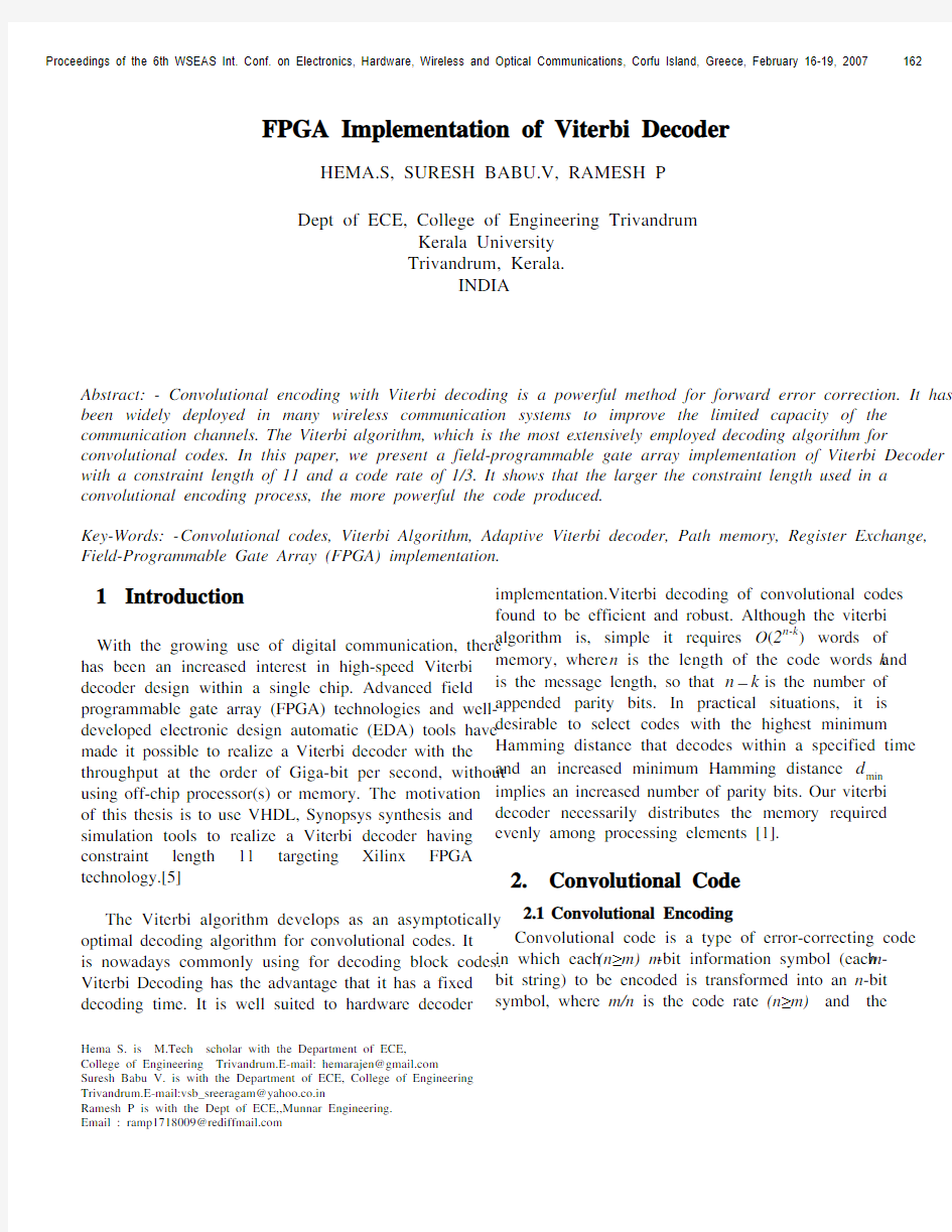
transformation is a function of the last k information symbols, where K is the constraint length of the code. To convolutionally encode data, start with k memory registers, each holding 1 input bit. Unless otherwise specified, all memory registers start with a value of 0.The encoder has n modulo-2 adders, and n generator polynomials—one for each adder (see figure1).An input bit m1is fed into the leftmost register. Using the generator polynomials and the existing values in the remaining registers, the encoder outputs n bits [1].
Figure 1: The rate ? Convolutional encoder
2.2Viterbi Algorithm
A. J. Viterbi proposed an algorithm as an ‘asymptotically optimum’ approach to the decoding of convolutional codes in memory-less noise. The Viterbi algorithm (VA) is knows as a maximum likelihood (ML)-decoding algorithm for convolutional codes. Maximum likelihood decoding means finding the code branch in the code trellis that was most likely to be transmitted. Therefore, maximum likelihood decoding is based on calculating the hamming distances for each branch forming encode word. The most likely path through the trellis will maximize this metric.[7]
Viterbi algorithm performs ML decoding by reducing its complexity. It eliminates least likely trellis path at each transmission stage and reduce decoding complexity with early rejection of unlike pathes.Viterbi algorithm gets its efficiency via concentrating on survival paths of the trellis. The Viterbi algorithm is an optimum algorithm for estimating the state sequence of a finite state process, given a set of noisy observations.[2]
The implementation of the VA consists of three parts: branch metric computation, path metric updating, and survivor sequence generation. The path metric computation unit computes a number of recursive equations. In a Viterbi decoder (VD) for an N-state convolutional code, N recursive equations are computed at each time step (N = 2k-1, k= constraint length). [12] Existing high-speed architectures use one processor per recursion equation. The main drawback of these Viterbi Decoders is that they are very expensive in terms of chip area. In current implementations, at least a single chip is dedicated to the hardware realization of the Viterbi decoding algorithm The novel scheduling scheme allows cutting back chip area dramatically with almost no loss in computation speed.[15]
3. Viterbi Decoder
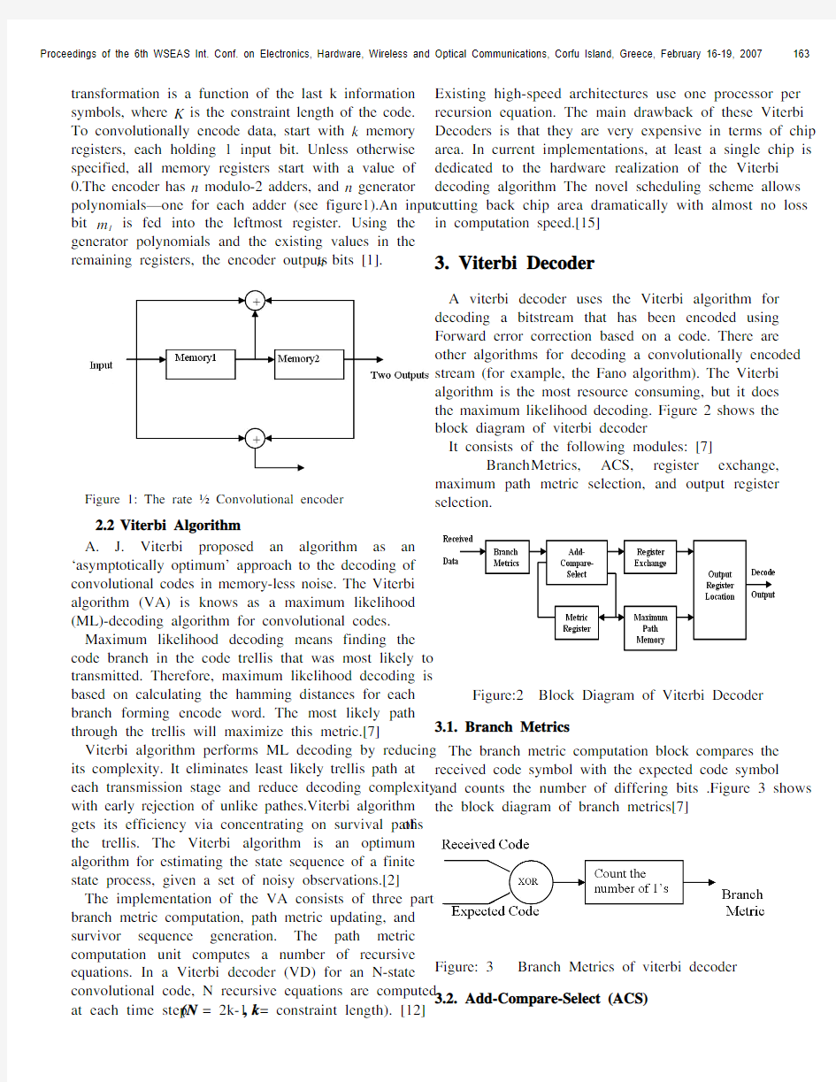
A viterbi decoder uses the Viterbi algorithm for decoding a bitstream that has been encoded using Forward error correction based on a code. There are other algorithms for decoding a convolutionally encoded stream (for example, the Fano algorithm). The Viterbi algorithm is the most resource consuming, but it does the maximum likelihood decoding. Figure 2 shows the block diagram of viterbi decoder
It consists of the following modules: [7]
Branch Metrics, ACS, register exchange, maximum path metric selection, and output register
selection.
Figure:2 Block Diagram of Viterbi Decoder
3.1. Branch Metrics
The branch metric computation block compares the received code symbol with the expected code symbol and counts the number of differing bits .Figure 3 shows
the block diagram of branch metrics[7]
Figure: 3 Branch Metrics of viterbi decoder
3.2. Add-Compare-Select (ACS)
The two adders compute the partial path metric of
each branch, the comparator compares the two partial metrics, and the selector selects an appropriate branch. The new partial path metric updates the state metric of state, and the survivor path-recording block records the survivor path.[7]
Figure 4 shows the block diagram of ACS block
Figure:4 ACS block
3.3. Path Metric Calculation and Storage The ACS circuit consisting of adders, a comparator, a selector, and several registers calculates the path metric of each convolutional code state. The number of “states” N, of a convolutional encoder which generates n encoded bits is a function of the constraint length K and input bits b .The path metric calculations just assigned the measurement functions to each state, but the actual Viterbi decisions on encoder states is based on a traceback operation to find the path of states. The important characteristic is that if every state from a current time is follow backwards through its maximum likelihood path, all of the paths converge at a point somewhere previous in time. This is how traceback decisively determines the state of the encoder at a given time, by showing that there is no better choice for an encoder state given the global maximum likelihood path.[6]
3.4 .Register-exchange and Traceback
The register-exchange approach assigns a register to each state. The register records the decoded output sequence along the path starting from the initial state to the final state, which is same as the initial state. This approach eliminates the need to traceback, since the register of the final state contains the decoded output sequence. Hence, the approach may offer a high-speed operation, but it is not power efficient due to the need to copy all the registers in a stage to the next stage.[10] The other approach called traceback records the survivor branch of each state. It is possible to traceback the survivor path provided the survivor branch of each state is known. While following the survivor path, the decoded output bit is ‘0’ (‘1’) whenever it encounters an even (odd) state. A flip-flop is assign to each state to
store the survivor branch and the flip-flop records ‘1’ (‘0’) if the survivor branch is the upper (lower) path. [6] 3.4.1) Traceback read (tb)
There are three types of operations performed inside a TB decoder:
This is one of the two read operations and consists of reading a bit and interpreting this bit in conjunction with the present state number as a pointer that indicates the previous state number (i.e. state number of the predecessor) .[4]
3.4.2) Decode read (dc)
This operation proceeds in exactly the same fashion as the traceback operation, but operates on older data, with the state number of the first decode read in a memory bank being determined by the previously completed traceback. Pointer values from this operation are the decoded values and are sent to the bit-order reversing circuit.
3.4.3) Writing new data (wr)
The decisions made by the ACS write into locations corresponding to the states. The write pointer advances forward as ACS operations move from one stage to the next in the trellis, and data are written to locations just freed by the decode read operation . 3.4.5) Selective Update and Shift Update
It is possible to form registers by collecting the flip-flops in the vertical direction or in the horizontal direction. When a register is formed in vertical direction, it is referred to as “selective update”. When a register is formed in horizontal direction, it is referred to as “shift update”. In selective update, the survivor path information is filling from the left register to the right register as the time progresses. In contrast, survivor path information is applied to the least significant bits of all the registers in “shift update”. Then all the registers perform a shift left operation. Hence, each register in the shift update method fills in survivor path information from the least significant bit toward the most significant bit.[9]
3.4.6) Survivor Path Memory
To implement the survivor path memory architecture, three types of path memory management schemes are commonly used: register-exchange (RE), trace-back (TB), and RE-TB-combined. The RE approach is suitable for fast decoders, but occupies large silicon real estate and consumes lots of power. On the other hand,
the TB path memory usually consumes less power, but is slower than its RE counterpart, or requires a clock rate higher than the decoding throughput. The RE-TB-combined approach, is a good alternative to the RE approach for high-speed applications. [7]
4. The Field Programmable Gate Array (FPGA)
A Field Programmable Gate Array (FPGA) is a semiconductor device containing programmable logic components and programmable interconnects. The programmable logic components can be programmed to duplicate the functionality of basic logic gates such as AND, OR, XOR, NOT or more complex combinational functions such as decoders or simple math functions. In most FPGAs, these programmable logic components (or logic blocks, in FPGA parlance) also include memory elements, which may be simple flip-flops or more complete blocks of memories. Each process is assigned to a different block of the FPGA and operates independently. A shared register between the processors implements the arcs, which represent the transmission of the weights and paths for each state to another processor. All systems were implementing in behavioral VHDL.A synthesis tool is used to construct the RTL level VHDL for the decoders. This synthesized unit is then simulated using a commercial simulation tool for VHDL.In VHDL the initial conditions such as the location of the weights and paths needed to update a state are readily coded and so don’t need to be calculated for each cycle of the decoding process. The received message is fan out into all the processors a bit at a time and this is the logical clock for the machine. On receiving each input bit, each processor reads the shared registers, updates the weights and paths and writes the results to the shared registers. [11]
FPGAs originally began as competitors to CPLDs and competed in a similar space, that of glue logic for PCBs. As their size, capabilities and speed increase, they began to take over larger and larger functions to the state where they are now market as competitors for full systems on chips. They now find applications in any area or algorithm that can make use of the massive parallelism offered by their architecture.[2]
The typical basic architecture consists of an array of configurable logic blocks (CLBs) and routing channels. Multiple I/O pads may fit into the height of one row or the width of one column. Generally, all the routing channels have the same width (number of wires).
An application circuit must be map into an FPGA with adequate resources. The typical basic architecture consists of an array of configurable logic blocks (CLBs) and routing channels. Multiple I/O pads may fit into the height of one row or the width of one column. Generally, all the routing channels have the same width (number of wires). [13]
FPGAs are an extremely valuable tool in learning VLSI design. While the traditional techniques of full- and semi-custom design certainly have their places for analog, high performance or complex applications, the prospect of putting “their” chip to the decisive test of a real hardware environment motivates students tremendously. [10]
To define the behavior of the FPGA the user provides a hardware description language (HDL) or a schematic design. Common HDLs are VHDL and Verilog. Then, using an electronic design automation tool, a technology-mapped netlist generates. The netlist can then be fitted to the actual FPGA architecture using a process called place-and-route, usually performed by the FPGA Company’s proprietary place-and-route software. The user will validate the map, place and route results via timing analysis, simulation, and other verification methodologies. Once the design and validation process is complete, the binary file generated (also using the FPGA company's proprietary software) is used to (re)configure the FPGA device. Figure: 5 show the design flow of FPGA. [2]
Figure: 5 Design flow of FPGA
To simplify the design of complex systems in FPGAs, there exist libraries of predefined complex functions and circuits that have been tested and optimized to speed up the design process. These predefined circuits are called IP cores, and are available from FPGA vendors and third-party IP suppliers (rarely free and typically released under proprietary licenses).
In a typical design flow, an FPGA application developer will simulate the design at multiple stages throughout the design process. Initially the RTL description in VHDL or Verilog is simulated by creating test benches to stimulate the system and observe results. Then, after the synthesis engine has mapped the design to a netlist, the netlist is translated to a gate level description where simulation is repeated to confirm the synthesis proceeded without errors. Finally, the design is laid out in the FPGA at which point propagation delays can be added and the simulation run again with these values back annotated onto the netlist.The typical FPGA logic block consists of a 4-input lookup table (LUT), and a flip-flop, as shown in Figure 6.[3]
Figure:6 Logic Block of FPGA
5. Conclusion
In this paper, a Viterbi algorithm based on the strongly connected trellis decoding of binary convolutional codes has been presented. The use of error-correcting codes has proven to be an effective way to overcome data corruption in digital communication channels. The adaptive Viterbi decoders are modeled using VHDL, and post synthesized by Xilinx Design Manager FPGA logic. The design simulations have been done based on both the VHDL codes at RTL and the VHDL codes generated by Xilinx design manager after post synthesis.
We can implement a higher performance Viterbi decoder with such as pipelining or interleaving. So in the future, with Pipeline or interleave the ACS and the trace-back and output decode block, we can make it better.
References
[1].”FPGA Design and Implementation of a Low-Power
Systolic Array-Based Adaptive Viterbi
Decoder”,IEEE Transactions on circuits and
systemsi: regular papers, vol. 52, no. 2, February
2005.
[2]. ”A Parallel Viterbi Decoder for Block Cyclic and
Convolution Codes”, Department of Electronics
and Computer Science, University of Southampton.
April 2006
[3]. ”A Dynamically Reconfigurable Adaptive Viterbi
Decoder”, International Symposium on FPGA
2002.
[4]. ”A Reconfigurable, Power-Efficient Adaptive
Viterbi Decoder”, This work was sponsored by
National Science Foundation grants.
[5]. X.Wang and S.B.Wicker,”An Artificial Neural
Net Viterbi Decoder,” IEEE
https://www.doczj.com/doc/cc6359940.html,munications,vol.44,no.2,pp.165-
171,February 1996.
[6]. D. Garrett and M. Stan, ” Low power architecture
of the soft-output Viterbi algorithm,”Electronic-
Letters, Proceeding 98 for ISLEPD 98, p 262-
267, 1998.
[7]. ”RTL implementation of Viterbi decoder”, Dept. of
Computer Engineering at Linkpings universitet.June 2006
[8]. Ranjan Bose ,“Information theory coding and
Cryptography”, McGraw-Hill.
[9]. G. Marcone and E. Zincolini. ”An efficient neural
decoder for convolutional codes.” European Trans.Telecomm.,6(4):439-445, July-August 1995.
[10]. J.G. Proakis. ”Digital Communications.”
McGraw-Hill,second edition, 1989.
[11]. A. J. Viterbi,”Convolutional codes and their
performance in communication systems,” IEEE
Trans. Commun., vol. COM-19, pp. 751 -772,Oct.,
1971.
[12]. LM Dong, SONG Wentao, LIU Xingzhao, LUO
Hanwen, XU Youyun, ZHANG Wenjun ”Neural Networks Based Parallel Viterbi Decoder by Hybrid Design” Department of Electronic Engineering, Shanghai Jiaotong University. [13]. C. B. Shung, H-D. Lin, R. Cypher, P. H. Siege1
and H. K. Thapar, ”Area-efficient architecture for the Viterbi algorithm Part 11: Applications,” IEEE Trans. Commun.,vol. 41, pp. 802-807, May 1993.
[14]. Shuji Kubota, Shuzo Kato, Member, IEEE, and
Tsunehachi Ishitani, ”Novel Viterbi Decoder VLSI Implementation and its Performance.”
IEEE Transactions on Communications, VOL. 41, NO. 8, AUGUST 1993.
[15]. Stevan M. Berber, Paul J. Secker, Zoran A.
Salcic, ”Theory and application of neural networks for 1/n rate convolutional decoders”,School of Engineering, The Department of Electrical and Computer Engineering, The University of Auckland,New Zealand.14 July 2005
(n,k,N)卷积码的维特比译码算法实现#include
2010年12月(上) Viterbi 译码的Matlab 实现 张慧 (盐城卫生职业技术学院,江苏盐城 224006) [摘要]本文主要介绍了Viterbi 译码是一种最大似然译码算法,是卷积编码的最佳译码算法。本文主要是以(2,1,2)卷积码为例,介 绍了Viterbi 译码的原理和过程,并用Matlab 进行仿真。[关键词]卷积码;Viterbi 译码 1卷积码的类型 卷积码的译码基本上可划分为两大类型:代数译码和概率译码,其中概率译码是实际中最常采用的卷积码译码方法。 2Viterbi 译码 Viterbi 译码是由Viterbi 在1967年提出的一种概率译码,其实质是最大似然译码,是卷积码的最佳译码算法。它利用编码网格图的特殊结构,降低了计算的复杂性。该算法考虑的是,去除不可能成为最大似然选择对象的网格图上的路径,即,如果有两条路径到达同一状态,则具有最佳量度的路径被选中,称为幸存路径( surviving path )。对所有状态都将进行这样的选路操作,译码器不断在网格图上深入,通过去除可能性最小的路径实现判决。较早地抛弃不可能的路径降低了译码器的复杂性。 为了更具体的理解Viterbi 译码的过程,我们以(2,1,2)卷积码为例,为简化讨论,假设信道为BSC 信道。译码过程的前几步如下:假定输入数据序列m ,码字U ,接收序列Z ,如图1所示,并假设译码器确知网格图的初始状态。 图1 时刻t 1接收到的码元是11,从状态00出发只有两种状态转移方向,00和10,如图a 所示。状态转换的分支量度是2;状态转换的分支径量度是0。时刻t 2从每个状态出发都有两种可能的分支,如图b 所示。这些分支的累积量度标识为状态量度┎a ,┎b ,┎c ,┎d ,与各自的结束状态相对应。同样地,图c 中时刻t 3从每个状态出发都有两个分支,因此,时刻时到达每个状态的路径都有两条,这两条路径中,累积路径量度较大的将被舍弃。如果这两条路径的路径量度恰好相等,则任意舍弃其中一条路径。到各个状态的幸存路径如图d 所示。译码过程进行到此时,时刻t 1和t 2之间仅有一条幸存路径,称为公共支(com-mon stem )。因此这时译码器可以判决时刻t 1和t 2之间的状态转移是00→10;因为这个状态转移是由输入比特1产生的,所以译码器输出1作为第一位译码比特。由此可以看出,用实线表示输入比特0,虚线表示输入比特1,可以为幸存路径译码带来很大的便利。注意,只有当路径量度计算进行到网格图较深处时,才产生第一位译码比特。在典型的译码器实现中,这代表了大约是约束长度5倍的译码延迟。 图2幸存路径选择 在译码过程的每—步,到达每个状态的可能路径总有两条,通过比较路径量度舍弃其中一条。图e 给出了译码过程的下一步:在时刻t 5到达各个状态的路径都有两条,其中一条被舍弃;图f 是时刻t 5的幸存路径。注意,此例中尚不能对第二位输入数据比特做出判决,因为在时刻t 2离开状态10的路径仍为两条。图g 中的时刻t 6同样有路径合并,图h 是时刻t 6的幸存路径,可见编码器输出的第二位译码比特是1,对应了时刻t 2和t 3之间的幸存路径。译码器在网格图上继续上述过程,通过不断舍弃路径直至仅剩一条,来对输入数据比特做出判决。 网格图的删减(通过路径的合并)确保了路径数不会超过状态数。对于此例的情况,可证明在图b 、d 、f 、h 中,每次删减后都只有4条路径。而对于未使用维特比算法的最大似然序列彻底比较法,其可能路径数(代表可能序列数)是序列长度的指数函数。对于分支字长为L 的二进制码字序列,共有2L 种可能的序列。下面我们用Matlab 函数viterbi (G,k,channel_output )来产生输入序列经Viterbi 译码器得到的输出序列,并将结果与输入卷积码编码器的信息序列进行比较。在这里,G =g ,k=k0,channel_output=output 。用Matlab 函数得到的译码输出为10011100110000111,这与我们经过理论分析得出的结果是一致的。 我们用subplot 函数将译码器最终的输出结果与(下转第261页) 250
编号: 《DSP技术与应用》课程论文卷积码的维特比译码的分析与实现 论文作者姓名:______ ______ 作者学号:___ ______ 所在学院: 所学专业:_____ ___ 导师姓名职称:__ _ 论文完成时间: _
目录 摘要: (1) 0 前言 (2) 1 理论基础 (2) 1.1信道理论基础 (2) 1.2差错控制技术 (3) 1.3纠错编码 (4) 1.4线性分组码 (5) 2 卷积码编码 (7) 2.1 卷积码概要 (7) 2.2 卷积码编码器 (8) 2.3卷积码的图解表示 (8) 2.4 卷积码的解析表示 (11) 3 卷积码的译码 (14) 3.1 维特比译码 (15) 3.2 代数译码 (17) 3.3 门限译码 (18) 4 维特比译码器实现 (18) 4.1 TMS320C54 系列DSP概述 (18) 4.2 Viterbi译码器的DSP实现 (19) 4.3 实现结果 (21) 5 结论 (21) 参考文献 (22) II
卷积码的维特比译码的分析与实现 摘要: 针对数据传输过程中的误码问题,本文论述了提高数据传输质量的一些编码及译码的实现问题。自P.Elias 首次提出卷积码编码以来,这一编码技术至今仍显示出强大的生命力。在与分组码同样的码率R 和设备复杂性的条件下,无论从理论上还是从实际上均己证明卷积码的性能至少不比分组码差,且实现最佳和准最佳译码也较分组码容易。目前,卷积码已广泛应用在无线通信标准中,其维特比译码则利用码树的重复性结构,对最大似然译码算法进行了简化。本文所做的主要工作: 首先对信道编码技术进行了研究,根据信道中可能出现的噪声等问题对卷积码编码方法进行了主要阐释。 其次,对卷积码维特比译码器的实现算法进行了研究,完成了译码器的软件设计。 最后,结合实例,采用DSP芯片实现卷积码的维特比译码算法的仿真和运行。 关键词: 卷积码维特比译码DSP Convolutional codes and Viterbi decoding analysis and realization Zhang Yi-Fei (School of Physics and Electronics, Henan University, Henan Kaifeng 475004, China) Abstract: Considering the error bit problem during data transmission,this thesis discussed some codings and decoders,aiming at enhancing transmission performance. From P.Elias first gave the concept of convolutional code, it has show its’ great advantage. Under the same condition and the same rate of block code, the performance of convolutional code is better than block code, and it’s easier to implement the best decoding.Convolutional codes have been widely used in wireless communication standards, the V iterbi decoding using the repetitive structure of the code tree, the maximum likelihood decoding algorithm has been simplified. Major work done in this article: First, the channel coding techniques have been studied, the main interpretation of the convolutional code encoding method according to the channel may be noise and other issues. Secondly, the convolutional code V iterbi decoder algorithm has been studied, the software design of the decoder. Finally, with examples, simulation and operation of the DSP chip convolutional codes, Viterbi decoding algorithm. 1
BUPT 卷积码编码及Viterbi译码 班级:07114 学号:070422 姓名:吴希龙 指导老师:彭岳星 邮箱:FusionBupt@https://www.doczj.com/doc/cc6359940.html,
1. 序言 卷积码最早于1955年由Elias 提出,稍后,1957年Wozencraft 提出了一种有效地译码方法即序列译码。1963年Massey 提出了一种性能稍差但是比较实用的门限译码方法,使得卷积码开始走向实用化。而后1967年Viterbi 提出了最大似然译码算法,它对存储级数较小的卷积码很容易实现,被称作Viterbi 译码算法,广泛的应用于现代通信中。 2. 卷积码编码及译码原理 2.1 卷积码编码原理 卷积码是一种性能优越的信道编码,它的编码器和解码器都比较易于实现,同时还具有较强的纠错能力,这使得它的使用越来越广泛。卷积码一般表示为(n,k,K)的形式,即将k 各信息比特编码为n 个比特的码组,K 为编码约束长度,说明编码过程中相互约束的码段个数。卷积码编码后的n 各码元不经与当前组的k 个信息比特有关,还与前K-1个输入组的信息比特有关。编码过程中相互关联的码元有K*n 个。R=k/n 是编码效率。编码效率和约束长度是衡量卷积码的两个重要参数。典型的卷积码一般选n,k 较小,但K 值可取较大(>10),以获得简单而高性能的卷积码。 卷积码的编码描述方式有很多种:冲激响应描述法、生成矩阵描述法、多项式乘积描述法、状态图描述,树图描述,网格图描述等。 2.1.1 卷积码解析表示法 卷积码的解析表示发大致可以分为离散卷积法,生成矩阵法,码多项式法。下面以离散卷积为例进行说明。 卷积码的编码器一般比较简单,为一个具有k 个输入端,n 个输出端,m 级移位寄存器的有限状态有记忆系统。下图所示为(2,1,7)卷积码的编码器。 若输入序列为u =(u 0u 1u 2u 3……), 则对应两个码字序列c ①=(c 0①c 1①c 2①c 3①……)和c ②=(c 0②c 1②c 2②c 3② ……) 相应的编码方程可写为c ①=u ?g ①,c ②=u ?g ②,c=(c ①,c ②)。 “?” 符号表示卷积运算,g ①,g ②表示编码器的两个冲激响应,即编码器的输出可以由输入序列和编码器的两个冲击响应卷积而得到,故称为卷积码。这里的冲激响应指:当输入为[1 0 0 0 0 … … ]序列时,所观察到的两个输出序列值。由于上图K 值为7,故冲激响应至
卷积码编码维特比译码实验设计报告 SUN 一、实验目的 掌握卷积码编码和维特比译码的基本原理,利用了卷积码的特性, 运用网格图和回溯以得到译码输出。 二、实验原理 1.卷积码是由连续输入的信息序列得到连续输出的已编码序列。其编码器将k个信息码元编为n个码元时,这n个码元不仅与当前段的k个信息有关,而且与前面的(m-1)段信息有关(m为编码的约束长度)。 2.一般地,最小距离d表明了卷积码在连续m段以内的距离特性,该码可以在m个连续码流内纠正(d-1)/2个错误。卷积码的纠错能力不仅与约束长度有关,还与采用的译码方式有关。 3. 维特比译码算法基本原理是将接收到的信号序列和所有可能的发送信号序列比较,选择其中汉明距离最小的序列认为是当前发送序列。卷积码的Viterbi 译码是根据接收码字序列寻找编码时通过网格图最佳路径的过程,找到最佳路径即完成了译码过程,并可以纠正接收码字中的错误比特。 4.所谓“最佳”, 是指最大后验条件概率:P( C/ R) = max [ P ( Cj/ R) ] , 一般来说, 信道模型并不使用后验条件概率,因此利用Beyes 公式、根据信道特性出结论:max[ P ( Cj/ R) ]与max[ P ( R/ Cj) ]等价。考虑到在系统实现中往往采用对数形式的运算,以求降低运算量,并且为求运算值为整数加入了修正因子a1 、a2 。令M ( R/ Cj) = log[ P ( R/ Cj) ] =Σa1 (log[ P( Rm/ Cmj ) ] + a2) 。其中, M 是组成序列的码字的个数。因此寻找最佳路径, 就变成寻找最大M( R/ Cj) , M( R/ Cj) 称为Cj 的分支路径量度,含义为发送Cj 而接收码元为R的似然度。 5.卷积码的viterbi译码是根据接收码字序列寻找编码时通过网格图最佳路径的过程,找到最佳路径即完成了译码过程并可以纠正接收码字中的错误比特。 三、实验代码 #include<> #include "" #define N 7 #include "" #include <> #include<> #define randomize() srand((unsigned)time(NULL)) encode( unsigned int *symbols, /*编码输出*/ unsigned int *data, /*编码输入*/ unsigned int nbytes, /*nbytes=n/16,n为实际输入码字的数目*/ unsigned int startstate /*定义初始化状态*/
译码主要部分 #include"stdafx.h" //#define DEBUG void deci2bin(int d, int size, int *b); int bin2deci(int *b, int size); int nxt_stat(int current_state, int input, int *memory_contents); void init_quantizer(void); void init_adaptive_quant(float es_ovr_n0); int soft_quant(float channel_symbol); int soft_metric(int data, int guess); int quantizer_table[256]; void sdvd(int g[2][K], float es_ovr_n0, long channel_length, float*channel_output_vector, int *decoder_output_matrix) { int i, j, l, ll; //循环控制变量 long t; //时间 int memory_contents[K]; //记录输入内容 int input[TWOTOTHEM][TWOTOTHEM]; //对当前状态以及下一个状态映射 int output[TWOTOTHEM][2]; //卷积码编码输出矩阵 int nextstate[TWOTOTHEM][2]; //下一个状态矩阵 int accum_err_metric[TWOTOTHEM][2]; //误差累计矩阵 int state_history[TWOTOTHEM][K * 5 + 1]; //历史状态表 int state_sequence[K * 5 + 1]; //状态序列 int *channel_output_matrix; //信道输出序列 int binary_output[2]; int branch_output[2]; //0或者1的输出分支 int m, n, number_of_states, depth_of_trellis, step, branch_metric, sh_ptr, sh_col, x, xx, h, hh, next_state, last_stop; n = 2; //1/2为卷积码传输数据的码率 m = K - 1;//寄存器个数 number_of_states = (int)pow(2.0, m);//状态个数number of states = 2^(K - 1) = 2^m depth_of_trellis = K * 5; for (i = 0; i < number_of_states; i++)
一种卷积码维特比译码算法的软件实现Ξ 张海勇1) 刘文予1) 芦东昕2) 吴 畏2) (华中科技大学电子与信息工程系1) 武汉 430074) (中兴通讯股份有限公司2) 深圳 518057) 摘 要 提出了数字通信系统中一种卷积码译码的软件实现方案,该方案应用软件技术实现了卷积码维特比译码器功能,在程序实现中充分利用了卷积码的特性,运用蝶形运算,周期性的回溯以得到译码输出。在程序设计上采用了一些宏定义等处理方法,可以提升运算速度,是一种软件方法的前向纠错编码技术。 关键词:卷积码 维特比译码算法 蝶形运算 回溯 中图分类号:TP31 A Soft w are Implementation of Viterbi Decoding Algorithm Zhang H aiyong1) Liu Wenyu1) Lu Dongxin2) Wu Wei2) (Dept.of Electronics&Information Engineering1),HUST,Wuhan430074) (ZTE Corporation2),Shenzhen518057) Abstract:A software implementation of a channel coding technology is presented,which realizes the functions of convolution2 al coding and Viterbi decoding.According to convolutional codes feature,this software uses butterfly algorithm which is defined as a macro,periodically traces back to get the decoding output,we also use some other methods in the program,can speed up the al2 gorithm,which belongs to a forward error correction coding technology. K ey w ords:convolutional code,Viterbi decoding algorithm,butterfly algorithm,trace back Class number:TP31 卷积码是由伊莱亚斯(Elias)于1954年首先提出来的。它充分利用了各组之间的相关性,本组的信息元不但决定本组的监督元,而且也参与决定以后若干组的监督元。同时在译码过程中,不但从该时刻所收到的码组中提取译码信息,而且还利用以后若干时刻内所收到的码组来提取有关信息。无论从理论上还是实际上均已证明其性能不差于分组码。在一些采用了前向纠错的系统里,如GS M/CDM A通信系统、卫星与空间通信系统里广泛采用了卷积码[1]。 卷积码译码器的设计是由高性能的复杂译码器开始的,如最初的序列译码,随着译码约束长度的增加,译码错误概率可达到非常小。后来慢慢地向低性能的简单译码器演化,对不太长的约束长度,维特比(V iterbi)算法是非常实用的。维特比算法是一种最大似然的译码方法。当编码约束度不太大(小于等于10)或者误码率要求不太高(约10-5)时[2],它的设备比较简单,用硬件译码计算速度很快。本文将给出一种用软件实现卷积码维特比译码算法的设计方法,针对译码中计算量最多的蝶形运算,采用宏定义的方式,并在计算度量长度时采用双数组计算,能够加快译码计算速度。 1 卷积码编码器的参数分析 卷积码把信源输出的信息序列以每段k0个码元进行分段,通过编码器输出长为n0的一个码段,该段(n0-k0)个校验元不仅与本段信息元有关,还与其前面m段信息元有关。卷积码可以用(n0,k0,K)表示,其中(K=m+1)为约束长度,串联的移位寄存器的数目以m表示,一个信息 Ξ收到本文时间:2004年12月2日
动态规划:卷积码的Viterbi译码算法 学院:网研院?姓名:xxx 学号:xxx一、动态规划原理 动态规划(dynamic programming)是运筹学的一个分支,是求解决策过程(decision process)最优化的数学方法。动态规划算法通常用于求解具有某种最优性质的问题。在这类问题中,可能会有许多可行解,每一个解都对应于一个值,我们希望找到具有最优值的解。动态规划算法与分治法类似,其基本思想也是将待求解问题分解成若干个子问题,先求解子问题,然后从这些子问题的解得到原问题的解。与分治法不同的是,适合于用动态规划求解的问题,经分解得到子问题往往不是互相独立的。若用分治法来解这类问题,则分解得到的子问题数目太多,有些子问题被重复计算了很多次。如果我们能够保存已解决的子问题的答案,而在需要时再找出已求得的答案,这样就可以避免大量的重复计算,节省时间。 动态规划程序设计是对解最优化问题的一种途径、一种方法,而不是一种特殊算法。不象搜索或数值计算那样,具有一个标准的数学表达式和明确清晰的解题方法。动态规划程序设计往往是针对一种最优化问题,由于各种问题的性质不同,确定最优解的条件也互不相同,因而动态规划的设计方法对不同的问题,有各具特色的解题方法,而不存在一种万能的动态规划算法,可以解决各类最优化问题。 二、卷积码的Viterbi译码算法简介 在介绍维特比译码算法之前,首先了解一下卷积码编码,它常常与维特比译码结合使用。(2,1,3)卷积码编码器是最常见的卷积码编码器,在本次实验中也使用了(2,1,3)卷积码编码器,下面介绍它的原理。 (2,1,3)卷积码是把信源输出的信息序列,以1个码元为一段,通过编码器输出长为2的一段码段。该码段的值不仅与当前输入码元有关,而且也与其之前的2个输入码元有关。如下图所示,输出out1是输入、第一个编码器存储的值和第二个编码器存储的值逻辑加操作的结果,输出out2是输入和第二个编码器存储的值逻辑加操作的结果。 (2,1,3)卷积码编码器
卷积码的维特比译码原理及仿真 摘 要 本课程设计主要解决对一个卷积码序列进行维特比(Viterbi)译码输出,并通过Matlab 软件进行设计与仿真,并进行误码率分析。 实验原理 QPSK :QPSK 是英文QuadraturePhaseShiftKeying 的缩略语简称, 意为正交相移键控,是一种数字调制方式。四相相移键控信号简称“QPSK ”。它分为绝对相移和相对相移两种。 卷积码:又称连环码,是由伊莱亚斯(P.elias)于1955年提出来的一种非分组码。积码将k 个信息比特编成n 个比特,但k 和n 通常很小,特别适合以串行形式进行传输,时延小。卷积码是在一个滑动的数据比特序列上进行模2和操作,从而生成一个比特码流。卷积码和分组码的根本区别在于,它不是把信息序列分组后再进行单独编码,而是由连续输入的信息序列得到连续输出的已编码序列。卷积码具有误码纠错的能力,首先被引入卫星和太空的通信中。NASA 标准(2,1,6)卷积码生成多项式为: 346 1345 6 2()1()1g D D D D D g D D D D D =++++=++++ 其卷积编码器为: 输入序列 + + 输出c1 输出c2 图1.1 K=7,码率为1/2的卷积码编码器
维特比译码:采用概率译码的基本思想是:把已接收序列与所有可能的发送序列做比较,选择其中码距最小的一个序列作为发送序列。如果接收到L 组信息比特,每个符号包括v 个比特。接收到的Lv 比特序列与2L 条路径进行比较,汉明距离最近的那一条路径被选择为最有可能被传输的路劲。当L 较大时,使得译码器难以实现。维特比算法则对上述概率译码做了简化,以至成为了一种实用化的概率算法。它并不是在网格图上一次比较所有可能的2kL 条路径(序列),而是接收一段,计算和比较一段,选择一段最大似然可能的码段,从而达到整个码序列是一个最大似然值得序列。 下面以图2.1的(2,1,3)卷积码编码器所编出的码为例,来说明维特比解码的方法和运作过程。为了能说明解码过程,这里给出该码的状态图,如图2.2所 示。维特比译码需要利用图来说明移码过程。根据卷积码画网格的方法,我们可以画出该码的网格图,如图2.3所示。该图设接收到的序列长度为8,所以画8个时间单位,图中分别标以0至7。这里设编码器从a 状态开始运作。该网格图的每一条路径都对应着不同的输入信息序列。由于所有可能输入信息序列共有2kL 个,因而网格图中所有可能的路径也为2L 条。这里节点a=00,b=10,c=01,d=11。 m j m j-1 m j-2 输出序列 m 1,m 2,…m j ,… y 1j y 2j 输入序列 00 a d 10 c b 11 00 11 01 01 10 图2.1 (2,1,3)卷积码编码器 图2.2 (2,1,3)卷积码状态图
卷积码编码和维特比译码的原理、性能与仿真分析 1.引言 卷积码的编码器是由一个有k位输入、n位输出,且具有m位移位寄存器构成的有限状态的有记忆系统,通常称它为时序网络。编码器的整体约束长度为v,是所有k个移位寄存器的长度之和。具有这样的编码器的卷积码称作[n,k,v]卷积码。对于一个(n,1,v)编码器,约束长度v等于存储级数m.卷积码是由k个信息比特编码成n(n>k)比特的码组,编码出的n比特码组值不仅与当前码字中的k个信息比特值有关,而且与其前面v个码组中的v*k个信息比特值有关。 卷积码有三种译码方式:序列译码、门限译码和概率译码。其中,概率译码根据最大似然译码原理在所有可能路径中求取与接收路径最相似的一条路径,具有最佳的纠错性能,维特比译码是概率译码中极重要的一种方式。 序列译码和门限译码则不一定能找出与接收路径最相似的一条路径。不同于维特比译码,门限译码与序列译码所需的计算量是可变的且对于给定信息分组的最终判决仅仅基于(m+1)个接收分组,而不是基于整个接收序列。 与维特比译码所使用的对数似然量度不同,序列译码所使用的量度为Fano量度。在接收序列受扰严重的情况下,序列译码的计算量大于维特比译码所需的固定计算量,虽然序列译码要求的平均计算次数通常小于维特比译码。在采用并行处理的情况下,维特比译码的速度会优于序列译码。在同样码率和存储级数的条件下,门限译码的性能比维特比译码低大约3dB. 维特比译码的数据输出方式有硬判决及软判决两种方式,本文选取生成多项式为561,753的(2,1,8)卷积码对硬判决的性能进行分析,并依据维特比译码的原理以及卷积码的特性,对卷积码编码和维特比译码过程在加性高斯白噪声(AWGN)信道下进行仿真,并且根据仿真结果对维特比译码(硬判决)的结果进行分析。由于卷积码的生成可以看做一个马尔科夫过程,因此,不同状态间的转移概率对描述这个过程有极关键的作用。本文则基于MATLAB对不同状态间的转移概率进行求解,从而更准确地分析维特比译码的性能。仿
译码器在数字通信中的应用 摘要:译码器可以用来实现组合电路,也可以用来实现码制转换。译码器就是把种代码转换为另一种代码的电路。随着现代电子技术的发展,译码器作为最基本的电子元器件之一,已广泛应用于数字通信系统中。 关键词:译码器,数字通信,维特比译码,Turbo码 1 引言 在数字电路中,能够实现译码功能的逻辑部件称为译码器(Decod6r)。实际上,译码器就是把一种代码转换为另一种代码的电路。译码器是一种组合逻辑电路。它的输入代码的组合将在某一个输出端产生特定的信号。译码是编码的逆过程,在编码时,每一种二进制代码状态都赋予了特定的含义,即都表示了一个确定的信号或者对象。把代码状态的特定含义翻译出来的过程称为译码,实现译码操作的电路称为译码器,或者说译码器是将输入二进制代码的状态翻译成输出信号,以表示其原来含义的电路。实际上,译码器就是把种代码转换为另一种代码的电路。随着现代电子技术的发展,译码器作为最基本的电子元器件之一,其应用领域越来越广泛,尤其是数字通信中的应用。 2原理 (1)译码器的原理 译码器的原理:用来表示输入变量状态的译码器是一种二进制译码器,输入输出代码之间的关系可由真值表表示。n个输入代码就有2n个输入状态,因此译码器就有2n个输出和输入状态相对应。每个输出的特定电位状态表示输入代码的一种组合。 (2)数字通信系统 数字通信系统是利用数字信号来传递信息的通信系统。如下图所示,数字通信主要涉及信编码和译码,信道编码与译码,同步及加密等等。 通信系统中信道编码的目的是增强数字信号的抗干扰能力。接受端的信道译码器按相应的逆规则进行解码,从中发现错误或纠正错误,提高通信系统的可靠性。纠错编码的基本思想是:在编码过程中,通过给所传输的信息设置附加的校验位,即增加其冗余度,使原来无规律或规律性不强的一组信息具有某种相关性;接收信息时再依据这种相关性译码,使编码信息具有检测或纠错性能,而用来检测或纠错的冗余码被称为纠错码。 (3)差错控制
维特比译码的介绍与仿真实现 维特比译码是将接收到的序列和所有可能的发送序列作比较,选择其中汉明距离最小的序列当作是现在的发送序列的一种算法。译码器从某个状态,例如从状态出发,每次向右延伸一个分支,并与接收数字相应分支进行比较,计算它们之间的距离,然后将计算所得距离加到被延伸路径的累积距离值中。对到达每个状态的各条路径的距离累积值进行比较,保留距离值最小的一条路径,称为幸存路径(当有两条以上取最小值时,可任取其中之一)。这种算法所保留的路径与接收序列之间的似然概率为最大,所以又称为最大似然译码。 所以,维特比译码的过程可以简单的理解为:接收端使用相同的网格图,从同一状态开始猜测发送端可能的编码序列,然后与接收到的码组比较,其中与接收到的码组最近的猜测序列即使为译码序列,也就是码距最小的序列。 设卷积码为(n, k, m) = (3, 1, 2)码,如下图:
那么对应的网格图为上图所示。 由网格图可见,沿路径每一级有4种状态a, b, c和d。每种状态只有两条路径可以到达。故4种状态共有8条到达路径。比较网格图中的这8条路径和接收序列之间的汉明距离。比较到达每个状态的两条路径的汉明距离,将距离小的一条路径保留,也就是幸存路径。这样,就剩下4条路径了。继续考察接收序列中的后继的比特,最后得出总的汉明距离最小的路径,也就是发送序列。 假设现在的发送信息位为1101 编码后的发送序列:111 110 010 100 001 011 000 接收序列:111 010 010 110 001 011 000 (红色为错码) 发送序列的约束长度为N = m + 1 = 3 最后的幸存路径画出的网格图示于下图中,图中粗线路径是距汉明离最小(等于2)的路径。 在上例中卷积码的约束长度为N = 3,需要存储和计算8条路径的参量。由此可见,维特比算法的复杂度随约束长度N按指数形式2N增长。故维特比算法适合约束长度较小(N 10)的编码。 卷积码的维特比译码是根据接收码字序列寻找编码时通过网格图最佳路径的过程,找到最佳路径即完成了译码过程,并可以纠正接收码字中的错误比特。维特比译码算法步骤如下描述: 1)根据接收码符号R,计算出相应的分支量度值BM(R/ Cj),j = 1 、2; 2)进入某一状态的2 条分支量度BM (R/ Cj)与其前状态路径量度PM累加 求和;
卷积编码和Viterbi译码 摘要 本文的目的是向读者介绍了前向纠错技术的卷积编码和Viterbi译码。前向纠错的目的(FEC)的是改善增加了一些精心设计的冗余信息,正在通过信道传输数据的通道容量。在添加这种冗余信息的过程称为信道编码。卷积编码和分组编码是两个主要的渠道形式编码。 简介 前向纠错的目的(FEC)的是改善增加了一些精心设计的冗余信息,正在通过信道传输数据的通道容量。在添加这种冗余信息的过程称为信道编码。卷积编码和分组编码是两个主要的渠道形式编码。卷积码串行数据操作,一次一个或数位。分组码操作比较大(通常,多达几百个字节的情侣)消息块。有很多有用的分组码和卷积多种,以及接收解码算法编码信息的DNA序列来恢复原来的各种数据。 卷积编码和Viterbi译码前向纠错技术,是一种特别适合于在其中一个已损坏的发射信号加性高斯白噪声(AWGN)的主要通道。你能想到的AWGN信道的噪声,其电压分布也随着时间的推移,可以说是用高斯,或正常,统计分布特征,即一钟形曲线。这个电压分布具有零均值和标准差这是一个信号与噪声比接收信号的信噪比(SNR)函数。让我们承担起接收到的信号电平是固定的时刻。这时如果信噪比高,噪声标 准偏差小,反之亦然。在数字通信,信噪比通常是衡量E b /N 的它代表噪声密度双面 能源每比特除以之一。 卷积码通常是描述使用两个参数:码率和约束长度。码率k/n,是表示为比特数为卷积编码器(十一)信道符号卷积编码器输出的编码器在给定的周期(N)的数量之比。约束长度参数,钾,表示该卷积编码器的“长度”,即有多少K位阶段提供饲料的组合逻辑,产生输出符号。 K是密切相关的参数米,这表明有多少位的输入编码器周期被保留,用于编码后第一次在卷积编码器输入的出现。的m参数可以被认为是编码器的记忆长度。在本教程中,并在此示例的源代码,我集中精力率1 / 2卷积码。 Viterbi译码是一种两个卷积编码与解码,其他类型的算法类型的顺序解码。序贯解码的优点,它可以执行得很好,长期约束卷积码的长度,但它有一个变量解码时间。
卷积码是1955年由Elias 等人提出的,是一种非常有前途的编码方法。我们在一些资料上可以找到关于分组码的一些介绍,分组码的实现是将编码信息分组单独进行编码,因此无论是在编码还是译码的过程中不同码组之间的码元无关。卷积码和分组码的根本区别在于,它不是把信息序列分组后再进行单独编码,而是由连续输 入的信息序列得到连续输出的已编码序列。即进行分组编码时,其本组中的n-k 个校验元仅与本组的k 个信息元有关,而与其它各组信息无关;但在卷积码中,其编 码器将k 个信息码元编为n 个码元时,这n 个码元不仅与当前段的k 个信息有关,而且与前面的(m -1)段信息有关(m 为编码的约束长度)。同样,在卷积码译码过程中,不仅从此时刻收到的码组中提取译码信息,而且还要利用以前或以后各时刻收到的码组中提取有关信息。而且卷积码的纠错能力随约束长度的增加而增强,差错率则随着约束长度增加而呈指数下降 。卷积码(n,k,m) 主要用来纠随机错误,它的码元与前后码元有一定的约束关系,编码复杂度可用编码约束长度m*n 来表示。一般地,最小距离d 表明了卷积码在连续m 段以内的距离特性,该码可以在m 个连续码流内纠正(d-1)/2个错误。卷积码的纠错能力不仅与约束长度有关,还与采用的译码方式有关。总之,由于n ,k 较小,且利用了各组之间的相关性,在同样的码率和设备的复杂性条件下,无论理论上还是实践上都证明:卷积码的性能至少不比分组码差。 编码原理[回目录] 以二元码为例,编码器如图。输入信息序列为u =(u 0, u 1,…),其多项式表示为u (x )=u 0+u 1x +…+u l x l +…。 编码器的连接可用多项式表示为g (1,1)(x )=1+x +x 2和 g (1,2)(x )=1+x 2,称为码的子生成多项式。它们的系数矢 量g (1,1)=(111)和g (1,2)=(101)称作码的子生成元。以子生成多项式为阵元构成的多项式矩阵G (x )= [g (1,1)(x ),g (1,2)(x )],称为码的生成多项式矩阵。由生成元构成的半无限矩阵 称为码的生成矩阵。其中(11,10,11)是由g (1,1)和g (1,2)交叉连接构成。编码器输出序列为c =u ·G ,称为码序 列,其多项式表示为c (x ),它可看作是两个子码序列c (1)(x )和c (2)(x )经过合路开关S 合成的,其中c (1)(x )=u (x )g (1,1)(x )和c (2)(x )=u (x )g (1,2)(x ),它们分别是信息序列和相应子生成元的卷积,卷积码由此得名。 在一般情况下,输入信息序列经过一个时分开关被分成k 0个子序列,分别以u (x )表示,其中i =1,2,…k 0,即u (x )=[ u (x ),…, u (x )]。编码器的结构由k 0×n 0阶生成多项式矩阵给定。输出码序列由n 0个子序列组成,即c (x )=[ c (x ), c (x ),…,c (x )],且c (x )=u (x )·G (x )。若m 是所有子生成多项式 g (x )中最高次式的次数,称这种码为(n 0,k 0,m ) 卷积码。 表示方法[回目录] 描述卷积码编码器过程的方法有很多,如矩阵法、多项式、码树和网格图等,这里我们主要介绍和卷积码编码器结构密切相关的多项式法,以及与卷积码译码密切相关的网格图法。 一种卷积码编码器 卷积码编码器
这周空时码的老师布置了一个编程的作业,有一天晚上突然兴起,熬夜到2点多,把这个程序写完了,虽然这个程序写的不算简单,于我自己毕竟是自己还是挺喜欢的,同学说我这个编程思想可以有点受C++的影响,不过我看了他写的那个,发现他在巧用矩阵方面确实比我强一点。下面我把程序贴出来,并做一些简单的说明。 %维特比算法 clear all; close all; filename=['tempdata_viterbi_v']; PAM=[-3 -1 1 3]; N=10000; %产生序列的长度 %x=[-3 3 1 -1 3 -1 -1 1 3 -3]; %输入x x_path=ceil(4*rand(1,N)); for i=1:N x(i)=PAM(x_path(i)); end y=zeros(1,length(x)+1); %输出y path=zeros(length(y),4); %路径存储 L=zeros(length(y),4); %距离存储
d=zeros(1,4); %SNR_dB=1:2:20; %count=1; %计数器 for SNR_dB=1:20 %检验输入序列 for i=1:N switch x(i) case -3 case -1 case 1 case 3 otherwise error('wrong input.'); end end %关于状态转移表(不加入噪声)y(i+1)=0.8*x(i+1)-0.6*x(i) P=[PAM;PAM;PAM;PAM]; state=(0.8*P'-0.6*P); %生成状态转移表--取原表的转置,便于计算 n=randn(1,length(x)); %噪声 sigma=sqrt(5)*10^(-SNR_dB/20);
第27卷第1期遥 测 遥 控 Vol .27,№.12006年1月Journa l of Tele m etry,Track i n g,and Co mmand January 2006 一种维特比译码改进算法的研究 刘国芳, 程乃平 (装备指挥技术学院 北京 101416) 收稿日期:2005204212 收修改稿日期:2005207208 摘 要:介绍传统维特比译码算法的基本原理;根据卷积编码的原理,结合(2,1,7)卷积码的子网表,提出一种维特比译码的改进算法,仿真结果表明,改进算法是可行的;最后通过数据分析,得出该算法与传统的译码算法相比具有存储量小、译码延迟短的优点。该算法同样适用于其它的卷积编码。 关键词:卷积码; 维待比译码; 译码算法 中图分类号:T N911.21 文献标识码:A 文章编号:CN11-1780(2006)01-0030-03 前 言 为了提高系统传输的质量,克服数据传输错误,一般采用差错控制编码,卷积编码是一种很好的纠错 编码方法。它满足线性叠加原理,且子生成元不随时间变化;与之相应的维特比算法是加性高斯白噪声信 道下卷积码的最优译码算法[1] 。 维特比译码算法是1967年V iterbi 提出的一种译卷积码的最大似然译码算法。在码的约束度较小时,它的译码效率较高、速度较快,因此广泛应用于数传系统,特别是卫星通信系统中。传统的维特比算法中的回溯算法采用通用的存储器作为存储主体,存储幸存路径的格状连接关系,通过读写存储器来完成数据的写入和回溯输出。但其译码延时较长。针对此,本文提出(2,1,7)卷积编码的维特比译码回溯算法的改进算法,该算法克服了传统算法的不足,有效地减少了存储器的存储空间,缩短了译码延迟。 1 传统的维特比译码算法的基本原理 [2,3] 维特比算法可用网格图来表示,它是一个时间序列的状态图。图1是一个简单的表示两个状态的状态转移网格图。在n -1时刻,两个可能状态x 0、x 1根据输入的信息可能转移到n 时刻的两个状态0x 、1x 。维特比算法就是通过在网格图中寻找最小路径度量值来判决最大似然状态序列,幸存路径存储就是存储具有最小路径度量值的信息。在传统的算法中,幸存路径存储器的组织采用类似指针的方法,将幸存路径分成前序状态的幸存路径和指向前序状态的指针两部分。在幸存路径存储器写满后要进行截尾译码,截图1 两状态转移网格图 尾译码的过程就是找出当前时刻n 的所有状态中具有最小路径度量值的状态,这个状态对应的路径就是最大似然路径,然后根据存储的指针找到其n -1时刻的前序状态,再根据该状态存储的指针找到其n -2时刻的前序状态,直到找到起始状态为止,它所存储的信息即为译码输出。在该算法中,幸存路径存储器所存储的内容既包括路径的信息,又包括前序状态的指针,因而需要大量的存储空间。同时,每输出一个译码结果需要回溯整个译码深度(即读L 次存储器),因而降低了译码速度。 2 改进的维特比译码算法 (2,1,7)卷积码有27-1个状态,根据其编码原理,可以得出当旧状态输入分别为0和1时对应的输 出新状态和输出值,将旧状态与新状态以及输入输出值制成表1所示的(2,1,7)卷积码的子网表。表1