wk10Chap010_market risk

of Politically Exposed Person (PEP) relationships and networks, and is customisable to identify a variety of specific third-party risks.The platform enables:−Advanced name-matching algorithms−Rich data−Secondary matching−Fewer false positives−Faster match resolution−Batch upload−Ongoing rescreening−Superior relevant media content screening Leverage LSEG World-Check, software and servicesWorld-Check One combines World-Check with the next generation of screening software. The software is built to maximise our proprietary World-Check data, capitalising on the powerof multiple secondary identifiers and additional information fields. With Enhanced Due Diligence reports and our Screening Resolution Service, organisations can focus on the recordsthat matter most.Screening software designed for World-Check−LSEG World-Check−Single name checks for manual name checking−Initial and ongoing screening of millions of records−Batch Screening−API with Zero Footprint Screening−A user interface available in multiple languages−Watchlist Screening that enables the user to upload in-house and third-party lists to screen against −Media Check AI-powered negative media screening tool, which pinpoints the media content most relevant to helping you meet your regulatory and legislative compliance requirements also available as an optional add-on via the World-Check One API−Identify Ultimate Beneficial OwnershipPowered by market-leading Dun & Bradstreet UBO data, our opt-in feature UBO Check lets you search and screen for regulatory and reputational risk with World-Check Risk Intelligence, all on one platform−Improved workflowOur enhanced case management functionality facilitates better visibility and improved breakdownof records, to help speed up the remediation process−Vessel due diligenceWith IHS Maritime data, check vessels for ownership structure and IMOs, and screen for any sanction and/or regulatory risk with World-Check all on our Vessel Check feature−Identity VerificationIdentity Check enables organisations to verify the identity of individuals and businesses through adata-based identity verification approach, utilising independent and authoritative identity data sources.World-Check One benefits More precision World-Check One enables greater customisation and control at name-matching level to screen against specific lists and data sets, or specific fields within those data sets, such as gender, nationality and date of birth.Lowering false positives When combined with the configurable name-matching algorithms and filtering technology in World-Check One, multiple secondary identifiers in World-Check help to reduce false positives.Intelligent teamwork The case management tool enables managers to define customised workflow to route cases to the right individuals and specialist teams, thereby reducing cycle times, promoting speed and efficiency, and giving teams more time to focus on investigations of the highest concern.Get more done with less World-Check One is designed to reduce the burden of daily customer screening. Its customisable searches, reduced false positives, ongoing screening capability and improved workflow reduce cycle times.Streamline the screening processOur World-Check One API facilitates the integration oflarge volumes of information and advanced functionalities into existing workflows and internal systems. Thisincreases the operational efficiency of the screeningprocess for onboarding, Know Your Customer (KYC) and third-party risk due diligence.One solution to screen multiple listsWatchlist Screening allows users to upload internaland third-party lists to World-Check One and apply thematching logic to all data sets, ensuring minimisation offalse positives and consistency of results.More precise media screeningNegative media forms part of a best practice approach to customer due diligence and ongoing risk assessment. AI delivers next-generation media screening of unstructured media, along with improved relevancy of results andworkflow integration, to enable better decision-making.Audit trail* and reporting capabilitiesWorld-Check One provides an extensive auditingcapability, with date-stamped actions for the matchresolution process. It includes detailed reports that canbe used as part of management reporting and regulatory proof of due diligence.World-Check One delivers a more efficient approachBalancing the regulatory and operational burden requires organisations to take a more targeted approach towards customer due diligence. Firms often have to do more with less. They require moreefficiency from the tools, technology and operations that support customer due diligence.*Not applicable for clients that do not require an audit trail.World-Check One leveragesWorld-CheckFind hidden risk in business relationships and human networks.World-Check provides trusted information to help businesses comply with regulations and identify potential financial crime. Since its inception, World-Check has served the KYC and third-party screening needs of the world’s largest firms, simplifying day-to-day onboarding and monitoring decisions, and helping businesses comply with anti-money laundering and countering financing of terrorism legislation. World-Check data is sourced from the public domain, deduplicated, structured into individual reports and linked to associations or human networks. Each action is underpinned by a meticulous, regulated research process.In addition to 100 percent sanctions coverage, additional risk-based information is sourced from extensive global media research by more than 400 research analysts working in over 65 languages, covering 240 countries. Information is collated from an extensive network of thousands of reputable sources, including 700+ sanction, watch, regulatory and law enforcement lists, local and international government records, country-specific data sources, international adverse electronic and physical media searches, and English and foreign language data sources.Sophisticated softwareA unified platform approach to customer due diligence.Our highly scalable solution is built for single users or large teams to support a carefully targeted approach to screening during KYC onboarding, ongoing monitoring and rescreening cycles. The system makes remediation quicker and more intelligent, and is adaptable to meet regulation changes.Additional servicesWe help organisations to optimise their resources and reduce operational cost.Screening Resolution Service – Our service highlights positive and possible matches for any customer identification programme detecting heightened risk individuals and entities, screened againstWorld-Check.By using a managed service like Screening Resolution Service, you can reduce your cost of compliance and free up departments to focus their efforts on activities such as tracking and implementing regulatory change. LSEG Due Diligence Reports – Use our Due Diligence reports to help you comply with anti-money laundering, anti-bribery and corruption regulations, or ahead of a merger, acquisition or joint venture. Y ou can also use them for third-party risk assessment, onboarding decision-making and identifying beneficial ownership structures.Using only ethical and non-intrusive research methods, LSEG is committed to principles of integrity and accountability. Subjects are not aware when we carry out an investigation, and we never misrepresent our activities. LSEG has a dedicated risk and control team that performs regular audits of the service, and external accreditation to ISAE 3000 standard through Schellman & Company, LLC.LSEG World-Check One for Salesforce – World-Check One for Salesforce connects your customer and third-party data from Salesforce with our proprietary World-Check to help you decide whether to onboard the vast majority of entities being screened or use further due diligence.Collaboration toolsEnhanced enterprise-level case management capabilities facilitate work on cases with assigned colleagues and teams when investigating risk, to ensure all decisions and discussions are captured as part of your audit trail. Secondary matchingApply secondary matching rules at list level based on your approach. Greater control enables reduced false positives. User experienceProven user interface promotes minimum user interaction.Cross-team communicationLanguage capabilities, ideal for multinational companies and team remediation.Prove due diligenceEach step of the screening process is tracked and saved for auditing purposes. T o satisfy regulatory demands, organisations can retrieve a detailed report showing the decision-making process and the individuals involved during every stage of the remediation process.World-Check One’s easy-to-use interface helps compliance teams work more efficiently.454312LDA3267049/10-23。

投资学第10版习题答案08CHAPTER 8: INDEX MODELSPROBLEM SETS1. The advantage of the index model, compared to the Markowitzprocedure, is the vastly reduced number of estimates required. In addition, the large number of estimates required for the Markowitz procedure can result in large aggregate estimation errors whenimplementing the procedure. The disadvantage of the index modelarises from the model’s assumption that return residuals areuncorrelated. This assumption will be incorrect if the index used omits a significant risk factor.2. The trade-off entailed in departing from pure indexing in favor ofan actively managed portfolio is between the probability (or thepossibility) of superior performance against the certainty of additional management fees.3. The answer to this question can be seen from the formulas for w0(equation 8.20) and w* (equation 8.21). Other things held equal, w0 is smaller the greater the residual variance of a candidate asset for inclusion in the portfolio. Further, we see that regardless of beta, when w0 decreases, so does w*. Therefore, other things equal, the greater the residual variance of an asset, the smaller itsposition in the optimal risky portfolio. That is, increased firm- specific risk reduces the extent to which an active investor will be willing to depart from an indexed portfolio.4. The total risk premium equals: + (× Market risk premium). Wecall alpha a nonmarket return premium because it is the portion of the return premium that is independent of market performance.The Sharpe ratio indicates that a higher alpha makes a securitymore desirable. Alpha, the numerator of the Sharpe ratio, is afixed number that is not affected by the standard deviation ofreturns, the denominator of the Sharpe ratio. Hence, an increase in alpha increases the Sharpe ratio. Since the portfolio alpha is the portfolio-weighted average of the securities’ alphas, then,holding all other parameters fixed, an increase in a security’s alpha results in an increase in the portfolio Sharpe ratio.5. a. To optimize this portfolio one would need:n = 60 estimates of means n = 60 estimates of variances 770,122=-n n estimates of covariances Therefore, in total: 890,1232=+n n estimatesb.In a single index model: r i r f = α i + β i (r M – r f ) + e iEquivalently, using excess returns: R i = α i + β i R M + e i The variance of the rate of return can be decomposed into the components: (l) The variance due to the common market factor:22M i σβ (2) The variance due to firm specific unanticipated events: )(σ2i e In this model: σββ),(Cov j i j i r r = The number of parameter estimates is: n = 60 estimates of the mean E (r i ) n = 60 estimates of the sensitivity coefficient β i n = 60 estimates of the firm-specific variance σ2(e i ) 1 estimate of the market mean E (r M ) 1 estimate of the market variance 2M σ Therefore, in total, 182 estimates. The single index model reduces the total number of required estimates from 1,890 to 182. In general, the number of parameter estimates is reduced from: )23( to 232+???? ??+n n n 6. a. The standard deviation of each individual stock is given by: 2/1222)](β[σi M i i e σσ+=Since βA = 0.8, βB = 1.2, σ(e A) = 30%, σ(e B) = 40%, and σM = 22%, we get:σA = (0.82× 222 + 302 )1/2 = 34.78%σB = (1.22× 222 + 402 )1/2 = 47.93%b. The expected rate of return on a portfolio is the weighted average of the expected returns of the individual securities: E(r P ) = w A × E(r A ) + w B × E(r B ) + w f × r f E(r P )= (0.30 × 13%) + (0.45 × 18%) + (0.25 × 8%) = 14% The beta of a portfolio is similarly a weighted average of the betas of the individual securities: βP = w A × βA + w B × βB + w f × β f βP = (0.30 × 0.8) + (0.45 × 1.2) + (0.25 × 0.0) = 0.78 The variance o f this portfolio is: )(σβσ2222P M P P e +=σ where 22σβM P is the systematic component and )(2P e σis the nonsystematic component. Since the residuals (e i ) are uncorrelated, the nonsystematic variance is: 2222222()()()()P A A B B f f e w e w e w e σσσσ=?+?+? = (0.302 × 302 ) + (0.452 × 402 ) + (0.252 × 0) = 405 where σ2(e A ) and σ2(e B ) are the firm-specific (nonsystematic) variances of StocksA and B, and σ2(e f ), the nonsystematic variance of T-bills, is zero. The residual standard deviation of the po rtfolio is thus: σ(e P ) = (405)1/2 = 20.12% The total variance of the portfolio is then: 47.699405)2278.0(σ222=+?=P The total standard deviation is 26.45%.7. a.The two figures depict the stocks’ security characteri stic lines (SCL). Stock A has higher firm-specific risk because the deviations of the observations from the SCL are larger for Stock A than for Stock B. Deviations are measured by the vertical distance of each observation from the SCL.b. Beta is the slope of the SCL, which is the measure ofsystematic risk. The SCL for Stock B is steeper; hence Stock B’s systematic risk is greater.c. The R 2(or squared correlation coefficient) of the SCL is the ratio of the explained variance of the stock’s return to total variance, and the total variance is the sum of the explained variance plus the unexplained variance (the stock’s residual variance): )(σσβσβ222222i M i M i e R += Since the explained variance for Stock B is greater than for Stock A (the explained variance is 22σβM B , which is greater since its beta is higher), and its residual variance 2()B e σ is smaller, its R 2 is higher than Stock A’s.d.Alpha is the intercept of the SCL with the expected return axis. Stock A has a small positive alpha whereas Stock B has a negative alpha; hence, Stock A’s alpha is larger.e.The correlation coefficient is simply the square root of R 2,so Stock B’s correlation with the market is higher.8. a.Firm-specific risk is measured by the residual standard deviation. Thus, stock A has more firm-specific risk: 10.3% > 9.1%b.Market risk is measured by beta, the slope coefficient of the regression. A has a larger beta coefficient: 1.2 > 0.8c.R 2 measures the fraction of total variance of return explained by the market return. A’s R 2 is larger than B’s: 0.576 >0.436d.Rewriting the SCL equation in terms of total return (r ) rather than excess return (R ): ()(1)A f M f A f M r r r r r r r αβαββ-=+?-?=+?-+? The intercept is now equal to: (1)1%(1 1.2)f f r r αβ+?-=+?- Since r f = 6%, the intercept would be: 1%6%(1 1.2)1% 1.2%0.2%+-=-=-。

（完整版）投资学第10版习题答案05CHAPTER 5: RISK, RETURN, AND THE HISTORICALRECORDPROBLEM SETS1. The Fisher equation predicts that the nominal rate will equal the equilibriumreal rate plus the expected inflation rate. Hence, if the inflation rate increasesfrom 3% to 5% while there is no change in the real rate, then the nominal ratewill increase by 2%. On the other hand, it is possible that an increase in theexpected inflation rate would be accompanied by a change in the real rate ofinterest. While it is conceivable that the nominal interest rate could remainconstant as the inflation rate increased, implying that the real rate decreasedas inflation increased, this is not a likely scenario.2. If we assume that the distribution of returns remains reasonably stable overthe entire history, then a longer sample period (i.e., a larger sample) increasesthe precision of the estimate of the expected rate of return; this is aconsequence of the fact that the standard error decreases as the sample sizeincreases. However, if we assume that the mean of the distribution of returnsis changing over time but we are not in a position to determine the nature ofthis change, then the expected return must be estimated from a more recentpart of the historical period. In this scenario, we must determine how far back,historically, to go in selecting the relevant sample. Here, it is likely to bedisadvantageous to use the entire data set back to 1880.3. The true statements are (c) and (e). The explanations follow.Statement (c): Let σ = the annual standard deviation of the risky investmentsand 1σ= the standard deviation of the first investment alternative over the two-year period. Then:σσ?=21Therefore, the annualized standard deviation for the first investment alternative is equal to:σσσ<=221Statement (e): The first investment alternative is more attractive to investors with lower degrees of risk aversion. The first alternative (entailing a sequence of two identically distributed and uncorrelated risky investments) is riskierthan the second alternative (the risky investment followed by a risk-freeinvestment). Therefore, the first alternative is more attractive to investors with lower degrees of risk aversion. Notice, however, that if you mistakenlybelieved that time diversification can reduce the total risk of a sequence ofrisky investments, you would have been tempted to conclude that the firstalternative is less risky and therefore more attractive to more risk-averseinvestors. This is clearly not the case; the two-year standard deviation of thefirst alternative is greater than the two-year standard deviation of the secondalternative.4. For the money market fund, your holding-period return for the next yeardepends on the level of 30-day interest rates each month when the fund rolls over maturing securities. The one-year savings deposit offers a 7.5% holding period return for the year. If you forecast that the rate on money marketinstruments will increase significantly above the current 6% yield, then themoney market fund might result in a higher HPR than the savings deposit.The 20-year Treasury bond offers a yield to maturity of 9% per year, which is 150 basis points higher than the rate on the one-year savings deposit; however, you could earn a one-year HPR much less than 7.5% on the bond if long-term interest rates increase during the year. If Treasury bond yields rise above 9%, then the price of the bond will fall, and the resulting capital loss will wipe out some or all of the 9% return you would have earned if bond yields hadremained unchanged over the course of the year.5. a. If businesses reduce their capital spending, then they are likely todecrease their demand for funds. This will shift the demand curve inFigure 5.1 to the left and reduce the equilibrium real rate of interest.b. Increased household saving will shift the supply of funds curve to theright and cause real interest rates to fall.c. Open market purchases of U.S. Treasury securities by the FederalReserve Board are equivalent to an increase in the supply of funds (ashift of the supply curve to the right). The FED buys treasuries withcash from its own account or it issues certificates which trade likecash. As a result, there is an increase in the money supply, and theequilibrium real rate of interest will fall.6. a. The “Inflation-Plus” CD is the safer investment because it guarantees thepurchasing power of the investment. Using the approximation that the realrate equals the nominal rate minus the inflation rate, the CD provides a realrate of 1.5% regardless of the inflation rate.b. The expected return depends on the expected rate of inflation over the nextyear. If the expected rate of inflation is less than 3.5% then the conventionalCD offers a higher real return than the inflation-plus CD; if the expected rateof inflation is greater than 3.5%, then the opposite is true.c. If you expect the rate of inflation to be 3% over the next year, then theconventional CD offers you an expected real rate of return of 2%, which is0.5% higher than the real rate on the inflation-protected CD. But unless youknow that inflation will be 3% with certainty, the conventional CD is alsoriskier. The question of which is the better investment then depends on yourattitude towards risk versus return. You might choose to diversify and investpart of your funds in each.d. No. We cannot assume that the entire difference between the risk-freenominal rate (on conventional CDs) of 5% and the real risk-free rate (oninflation-protected CDs) of 1.5% is the expected rate of inflation. Part of thedifference is probably a risk premium associated with the uncertaintysurrounding the real rate of return on the conventional CDs. This impliesthat the expected rate of inflation is less than 3.5% per year.7. E(r) = [0.35 × 44.5%] + [0.30 × 14.0%] + [0.35 × (–16.5%)] = 14%σ2 = [0.35 × (44.5 – 14)2] + [0.30 × (14 – 14)2] + [0.35 × (–16.5 – 14)2] = 651.175 σ = 25.52%The mean is unchanged, but the standard deviation has increased, as theprobabilities of the high and low returns have increased.8. Probability distribution of price and one-year holding period return for a 30-year U.S. Treasury bond (which will have 29 years to maturity at year-end):Economy Probability YTM Price CapitalGainCouponInterest HPRBoom 0.20 11.0% $ 74.05 -$25.95 $8.00 -17.95% Normal growth 0.50 8.0 100.00 0.00 8.00 8.00 Recession 0.30 7.0 112.28 12.28 8.00 20.289. E(q) = (0 × 0.25) + (1 × 0.25) + (2 × 0.50) = 1.25σq = [0.25 × (0 – 1.25)2 + 0.25 × (1 – 1.25)2 + 0.50 × (2 – 1.25)2]1/2 = 0.8292 10. (a) With probability 0.9544, the value of a normally distributedvariable will fall within 2 standard deviations of the mean; that is,between –40% and 80%. Simply add and subtract 2 standarddeviations to and from the mean.11. From Table 5.4, the average risk premium for the period 7/1926-9/2012 was:12.34% per year.Adding 12.34% to the 3% risk-free interest rate, the expected annual HPR for the Big/Value portfolio is: 3.00% + 12.34% = 15.34%.No. The distributions from (01/1928–06/1970) and (07/1970–12/2012) periods have distinct characteristics due to systematic shocks to the economy and subsequent government intervention. While the returns from the two periods do not differ greatly, their respective distributions tell a different story. The standard deviation for all six portfolios is larger in the first period. Skew is also positive, but negative in the second, showing a greater likelihood of higher-than-normal returns in the right tail.Kurtosis is also markedly larger in the first period.13. a%88.5,0588.070.170.080.01111or i i rn i rn rr =-=+-=-++=b. rr ≈ rn - i = 80% - 70% = 10%Clearly, the approximation gives a real HPR that is too high.14. From Table 5.2, the average real rate on T-bills has been 0.52%.a. T-bills: 0.52% real rate + 3% inflation = 3.52%b. Expected return on Big/Value:3.52% T-bill rate + 12.34% historical risk premium = 15.86%c. The risk premium on stocks remains unchanged. A premium, thedifference between two rates, is a real value, unaffected by inflation.15. Real interest rates are expected to rise. The investment activity will shiftthe demand for funds curve (in Figure 5.1) to the right. Therefore theequilibrium real interest rate will increase.16. a. Probability distribution of the HPR on the stock market and put:STOCK PUT State of theEconomyProbability Ending Price + Dividend HPR Ending Value HPR Excellent0.25 $ 131.00 31.00% $ 0.00 -100% Good0.45 114.00 14.00 $ 0.00 -100 Poor0.25 93.25 ?6.75 $ 20.25 68.75 Crash 0.05 48.00 -52.00 $ 64.00 433.33Remember that the cost of the index fund is $100 per share, and the costof the put option is $12.b. The cost of one share of the index fund plus a put option is $112. Theprobability distribution of the HPR on the portfolio is:State of the Economy Probability Ending Price + Put + DividendHPRExcellent 0.25 $ 131.00 17.0%= (131 - 112)/112 Good 0.45 114.00 1.8= (114 - 112)/112 Poor 0.25 113.50 1.3= (113.50 - 112)/112 Crash0.05 112.00 0.0 = (112 - 112)/112 c. Buying the put option guarantees the investor a minimum HPR of 0.0% regardless of what happens to the stock's price. Thus, it offers insuranceagainst a price decline.17. The probability distribution of the dollar return on CD plus call option is:State of theEconomy Probability Ending Valueof CDEnding Valueof CallCombinedValueExcellent 0.25 $ 114.00 $16.50 $130.50Good 0.45 114.00 0.00 114.00Poor 0.25 114.00 0.00 114.00Crash 0.05 114.00 0.00 114.0018.a.Total return of the bond is (100/84.49)-1 = 0.1836. With t = 10, the annualrate on the real bond is (1 + EAR) = = 1.69%.b.With a per quarter yield of 2%, the annual yield is = 1.0824, or8.24%. The equivalent continuously compounding (cc) rate is ln(1+.0824)= .0792, or 7.92%. The risk-free rate is 3.55% with a cc rate of ln(1+.0355)= .0349, or 3.49%. The cc risk premium will equal .0792 - .0349 = .0443, or4.433%.c.The appropriate formula is ,where . Using solver or goal seek, setting thetarget cell to the known effective cc rate by changing the unknown variance(cc) rate, the equivalent standard deviation (cc) is 18.03% (excel mayyield slightly different solutions).d.The expected value of the excess return will grow by 120 months (12months over a 10-year horizon). Therefore the excess return will be 120 ×4.433% = 531.9%. The expected SD grows by the square root of timeresulting in 18.03% × = 197.5%. The resulting Sharpe ratio is531.9/197.5 = 2.6929. Normsdist (-2.6929) = .0035, or a .35% probabilityof shortfall over a 10-year horizon.CFA PROBLEMS1. The expected dollar return on the investment in equities is $18,000 (0.6 × $50,000 + 0.4×?$30,000) compared to the $5,000 expected return for T-bills. Therefore, the expected risk premium is $13,000.2. E(r) = [0.2 × (?25%)] + [0.3 × 10%] + [0.5 × 24%] =10%3. E(r X) = [0.2 × (?20%)] + [0.5 × 18%] + [0.3 × 50%] =20%E(r Y) = [0.2 × (?15%)] + [0.5 × 20%] + [0.3 × 10%] =10%4. σX2 = [0.2 × (– 20 – 20)2] + [0.5 × (18 – 20)2] + [0.3 × (50 – 20)2] = 592σX = 24.33%σY2 = [0.2 × (– 15 – 10)2] + [0.5 × (20 – 10)2] + [0.3 × (10 – 10)2] = 175σY = 13.23%5. E(r) = (0.9 × 20%) + (0.1 × 10%) =19% $1,900 in returns6. The probability that the economy will be neutral is 0.50, or 50%. Given aneutral economy, the stock will experience poor performance 30% of thetime. The probability of both poor stock performance and a neutral economy is therefore: 0.30 × 0.50 = 0.15 = 15%7. E(r) = (0.1 × 15%) + (0.6 × 13%) + (0.3 × 7%) = 11.4%。

赫尔期权、期货及其他衍生产品第10版框架知识点及课后习题解析背景介绍赫尔期权、期货及其他衍生产品是一本经典的金融学教材，已经出版了多个版本。

本文将对第10版的框架知识点进行详细介绍，并对课后习题进行解析。

框架知识点第1章期权与期权市场本章主要介绍了期权的基本概念和期权市场的基本特点。

其中包括期权的定义、期权的基本特征、期权的交易方式、期权市场的参与者和期权市场的发展趋势等内容。

第2章期权定价基础本章介绍了期权定价的基本理论。

其中包括无套利定价原理、布莱克-舒尔斯期权定价模型、期权的几何布朗运动模型和完全市场假设等内容。

此外，还介绍了期权定价模型的应用和限制。

第3章期权策略与风险管理本章介绍了期权策略的基本概念和常见的期权策略类型。

其中包括购买期权、卖出期权、期权组合策略和套利策略等内容。

此外，还介绍了期权风险管理的基本方法和相关的风险指标。

第4章期货市场与期货定价本章介绍了期货市场的基本原理和期货合约的定价方法。

其中包括期货市场的特点、期货合约的基本要素、期货定价的原理和期货定价模型等内容。

此外，还介绍了期货市场的参与者和期货交易的风险管理。

第5章期货交易策略与风险管理本章介绍了期货交易策略的基本原理和常用的期货交易策略类型。

其中包括多头策略、空头策略、套利策略和市场中性策略等内容。

此外，还介绍了期货交易的风险管理方法和基本的交易技巧。

第6章期货市场的运行与监管本章介绍了期货市场的运行机制和监管体系。

其中包括期货市场的交易流程、交易所的角色和功能、期货市场的风险管理和期货市场的监管机构等内容。

此外，还介绍了期货市场的监管规则和期货市场的发展趋势。

课后习题解析第1章期权与期权市场习题1：期权是一种金融衍生品，它的特点是什么？答：期权有两个基本特点，即灵活性和杠杆效应。

灵活性指的是期权可以灵活选择行权，可以在未来的某个时间点以特定的价格购买或者卖出标的资产。

杠杆效应指的是期权的价格相对于标的资产的价格波动比较大，可以获得倍数的投资回报。

CHAPTER 7: OPTIMAL RISKY PORTFOLIOSPROBLEM SETS1.(a) and (e). Short-term rates and labor issues are factors that are common to all firms and therefore must be considered as market risk factors. The remaining three factors are unique to this corporation and are not a part of market risk.2.(a) and (c). After real estate is added to the portfolio, there are four asset classes in the portfolio: stocks, bonds, cash, and real estate. Portfolio variance now includes a variance term for real estate returns and a covariance term for real estate returns with returns for each of the other three asset classes. Therefore, portfolio risk is affected by the variance (or standard deviation) of real estate returns and thecorrelation between real estate returns and returns for each of the other asset classes. (Note that the correlation between real estate returns and returns for cash is most likely zero.)3.(a) Answer (a) is valid because it provides the definition of the minimum variance portfolio.4.The parameters of the opportunity set are:E (r S ) = 20%, E (r B ) = 12%, σS = 30%, σB = 15%, ρ = 0.10From the standard deviations and the correlation coefficient we generate the covariance matrix [note that ]:(,)S B S B Cov r r ρσσ=⨯⨯Bonds StocksBonds 22545Stocks45900The minimum-variance portfolio is computed as follows:w Min (S ) =1739.0)452(22590045225)(Cov 2)(Cov 222=⨯-+-=-+-B S B S B S B ,r r ,r r σσσw Min (B ) = 1 - 0.1739 = 0.8261The minimum variance portfolio mean and standard deviation are:E (r Min ) = (0.1739 × .20) + (0.8261 × .12) = .1339 = 13.39%σMin = 2/12222)],(Cov 2[B S B S B B S S r r w w w w ++σσ= [(0.17392 ⨯ 900) + (0.82612 ⨯ 225) + (2 ⨯ 0.1739 ⨯ 0.8261 ⨯ 45)]1/2= 13.92%5.Proportion in Stock Fund Proportion in Bond FundExpectedReturn Standard Deviation 0.00%100.00%12.00%15.00%17.3982.6113.3913.92minimum variance 20.0080.0013.6013.9440.0060.0015.2015.7045.1654.8415.6116.54tangency portfolio60.0040.0016.8019.5380.0020.0018.4024.48100.000.0020.0030.00Graph shown below.6.The above graph indicates that the optimal portfolio is the tangency portfolio with expected return approximately 15.6% and standard deviation approximately 16.5%.7.The proportion of the optimal risky portfolio invested in the stock fund is given by:222[()][()](,)[()][()][()()](,)S f B B f S B S S f B B f S S f B f S B E r r E r r Cov r r w E r r E r r E r r E r r Cov r r σσσ-⨯--⨯=-⨯+-⨯--+-⨯ [(.20.08)225][(.12.08)45]0.4516[(.20.08)225][(.12.08)900][(.20.08.12.08)45]-⨯--⨯==-⨯+-⨯--+-⨯10.45160.5484B w =-=The mean and standard deviation of the optimal risky portfolio are:E (r P ) = (0.4516 × .20) + (0.5484 × .12) = .1561 = 15.61% σp = [(0.45162 ⨯ 900) + (0.54842 ⨯ 225) + (2 ⨯ 0.4516 ⨯ 0.5484 × 45)]1/2= 16.54%8.The reward-to-volatility ratio of the optimal CAL is:().1561.080.4601.1654p fpE r r σ--==9.a.If you require that your portfolio yield an expected return of 14%, then you can find the corresponding standard deviation from the optimal CAL. The equation for this CAL is:()().080.4601p fC f C CPE r r E r r σσσ-=+=+If E (r C ) is equal to 14%, then the standard deviation of the portfolio is 13.04%.b.To find the proportion invested in the T-bill fund, remember that the mean of the complete portfolio (i.e., 14%) is an average of the T-bill rate and theoptimal combination of stocks and bonds (P ). Let y be the proportion invested in the portfolio P . The mean of any portfolio along the optimal CAL is:()(1)()[()].08(.1561.08)C f P f P f E r y r y E r r y E r r y =-⨯+⨯=+⨯-=+⨯-Setting E (r C ) = 14% we find: y = 0.7884 and (1 − y ) = 0.2119 (the proportion invested in the T-bill fund).To find the proportions invested in each of the funds, multiply 0.7884 times the respective proportions of stocks and bonds in the optimal risky portfolio:Proportion of stocks in complete portfolio = 0.7884 ⨯ 0.4516 = 0.3560Proportion of bonds in complete portfolio = 0.7884 ⨯ 0.5484 = 0.4323ing only the stock and bond funds to achieve a portfolio expected return of 14%, we must find the appropriate proportion in the stock fund (w S ) and the appropriate proportion in the bond fund (w B = 1 − w S ) as follows:0.14 = 0.20 × w S + 0.12 × (1 − w S ) = 0.12 + 0.08 × w S ⇒ w S = 0.25So the proportions are 25% invested in the stock fund and 75% in the bond fund. The standard deviation of this portfolio will be:σP = [(0.252 ⨯ 900) + (0.752 ⨯ 225) + (2 ⨯ 0.25 ⨯ 0.75 ⨯ 45)]1/2 = 14.13%This is considerably greater than the standard deviation of 13.04% achieved using T-bills and the optimal portfolio.11.a.Standard Deviation(%)0.005.0010.0015.0020.0025.00010203040Even though it seems that gold is dominated by stocks, gold might still be an attractive asset to hold as a part of a portfolio. If the correlation between gold and stocks is sufficiently low, gold will be held as a component in a portfolio, specifically, the optimal tangency portfolio.b.If the correlation between gold and stocks equals +1, then no one would holdgold. The optimal CAL would be composed of bills and stocks only. Since theset of risk/return combinations of stocks and gold would plot as a straight linewith a negative slope (see the following graph), these combinations would bedominated by the stock portfolio. Of course, this situation could not persist. If noone desired gold, its price would fall and its expected rate of return wouldincrease until it became sufficiently attractive to include in a portfolio.ll12.Since Stock A and Stock B are perfectly negatively correlated, a risk-free portfoliocan be created and the rate of return for this portfolio, in equilibrium, will be therisk-free rate. To find the proportions of this portfolio [with the proportion w Ainvested in Stock A and w B = (1 – w A) invested in Stock B], set the standarddeviation equal to zero. With perfect negative correlation, the portfolio standarddeviation is:σP = Absolute value [w AσA-w BσB]0 = 5 × w A− [10 ⨯ (1 – w A)] ⇒w A = 0.6667The expected rate of return for this risk-free portfolio is:E(r) = (0.6667 × 10) + (0.3333 × 15) = 11.667%Therefore, the risk-free rate is: 11.667%13.False. If the borrowing and lending rates are not identical, then, depending on the tastes of the individuals (that is, the shape of their indifference curves), borrowers and lenders could have different optimal risky portfolios.14.False. The portfolio standard deviation equals the weighted average of the component-asset standard deviations only in the special case that all assets are perfectly positively correlated. Otherwise, as the formula for portfolio standard deviation shows, the portfolio standard deviation is less than the weighted average of the component-asset standard deviations. The portfolio variance is a weighted sum of the elements in the covariance matrix, with the products of the portfolio proportions as weights.15.The probability distribution is:ProbabilityRate of Return0.7100%0.3−50Mean = [0.7 × 100%] + [0.3 × (-50%)] = 55%Variance = [0.7 × (100 − 55)2] + [0.3 × (-50 − 55)2] = 4725Standard deviation = 47251/2 = 68.74%16.σP = 30 = y × σ = 40 × y ⇒ y = 0.75E (r P ) = 12 + 0.75(30 − 12) = 25.5%17.The correct choice is (c). Intuitively, we note that since all stocks have the same expected rate of return and standard deviation, we choose the stock that will result in lowest risk. This is the stock that has the lowest correlation with Stock A.More formally, we note that when all stocks have the same expected rate of return, the optimal portfolio for any risk-averse investor is the global minimum variance portfolio (G). When the portfolio is restricted to Stock A and one additional stock, the objective is to find G for any pair that includes Stock A, and then select the combination with the lowest variance. With two stocks, I and J, the formula for the weights in G is:)(1)(),(Cov 2),(Cov )(222I w J w r r r r I w Min Min J I J I J I J Min -=-+-=σσσSince all standard deviations are equal to 20%:(,)400and ()()0.5I J I J Min Min Cov r r w I w J ρσσρ====This intuitive result is an implication of a property of any efficient frontier, namely, that the covariances of the global minimum variance portfolio with all other assets on the frontier are identical and equal to its own variance. (Otherwise, additional diversification would further reduce the variance.) In this case, the standard deviation of G(I, J) reduces to:1/2()[200(1)]Min IJ G σρ=⨯+This leads to the intuitive result that the desired addition would be the stock with the lowest correlation with Stock A, which is Stock D. The optimal portfolio is equally invested in Stock A and Stock D, and the standard deviation is 17.03%.18.No, the answer to Problem 17 would not change, at least as long as investors are not risk lovers. Risk neutral investors would not care which portfolio they held since all portfolios have an expected return of 8%.19.Yes, the answers to Problems 17 and 18 would change. The efficient frontier of risky assets is horizontal at 8%, so the optimal CAL runs from the risk-free rate through G. This implies risk-averse investors will just hold Treasury bills.20.Rearrange the table (converting rows to columns) and compute serial correlation results in the following table:Nominal RatesFor example: to compute serial correlation in decade nominal returns for large-company stocks, we set up the following two columns in an Excel spreadsheet. Then, use the Excel function “CORREL” to calculate the correlation for the data.Decade Previous 1930s -1.25%18.36%1940s 9.11%-1.25%1950s 19.41%9.11%1960s7.84%19.41%f 1970s 5.90%7.84%1980s 17.60% 5.90%1990s 18.20%17.60%Note that each correlation is based on only seven observations, so we cannot arrive at any statistically significant conclusions. Looking at the results, however, it appears that, with the exception of large-company stocks, there is persistent serial correlation. (This conclusion changes when we turn to real rates in the next problem.)21.The table for real rates (using the approximation of subtracting a decade’s average inflation from the decade’s average nominal return) is:Real RatesWhile the serial correlation in decade nominal returns seems to be positive, it appears that real rates are serially uncorrelated. The decade time series (although again too short for any definitive conclusions) suggest that real rates of return are independent from decade to decade.22. The 3-year risk premium for the S&P portfolio is, the 3-year risk premium for the hedge fund(1+.05)3‒1=0.1576 or 15.76%portfolio is S&P 3-year standard deviation is 0(1+.1)3‒1=0.3310 or 33.10%. . The hedge fund 3-year standard deviation is 0. S&P Sharpe ratio is 15.76/34.64 = 0.4550, and thehedge fund Sharpe ratio is 33.10/60.62 = 0.5460.23.With a ρ = 0, the optimal asset allocation isW S &P =,15.76×60.622‒33.10×(0×34.64×60.62)15.76×60.622+33.10×34.642‒[15.76+33.10]×(0×34.64×60.62)=0.5932.W Hedge =1‒0.5932=0.4068With these weights,ne iEσp=.59322×34.642+.40682×60.622+2×.5932×.4068×(0×=0.3210 or 32.10%The resulting Sharpe ratio is 22.81/32.10 = 0.7108. Greta has a risk aversion of A=3, Therefore, she will investyof her wealth in this risky portfolio. The resulting investment composition will be S&P: 0.7138 59.32 = 43.78% and Hedge: 0.7138 40.68 = 30.02%. The remaining 26% will be invested in the risk-free asset.24. With ρ = 0.3, the annual covariance is .25. S&P 3-year standard deviation is . The hedge fund 3-year standard deviation is . Therefore, the 3-yearcovariance is 0.26. With a ρ=.3, the optimal asset allocation isW S &P =,15.76×60.622‒33.10×(.3×34.64×60.62)15.76×60.622+33.10×34.642‒[15.76+33.10]×(.3×34.64×60.62)=0.5545.W Hedge =1‒0.5545=0.4455With these weights,Eσp=.55452×34.642+.44552×60.622+2×.5545×.4455×(.3×=0.3755 or 37.55%The resulting Sharpe ratio is 23.49/37.55 = 0.6256. Notice that the higher covariance results in a poorer Sharpe ratio. Greta will investyof her wealth in this risky portfolio. The resulting investment composition will be S&P: 0.5554 55.45 =30.79% and hedge: 0.5554 44.55= 24.74%. The remaining 44.46% will be invested in the risk-free asset.CFA PROBLEMS 1.a.Restricting the portfolio to 20 stocks, rather than 40 to 50 stocks, will increase the risk of the portfolio, but it is possible that the increase in risk will beminimal. Suppose that, for instance, the 50 stocks in a universe have the same standard deviation (σ) and the correlations between each pair are identical, with correlation coefficient ρ. Then, the covariance between each pair of stocks would be ρσ2, and the variance of an equally weighted portfolio would be:222ρσ1σ1σnn n P -+=The effect of the reduction in n on the second term on the right-hand side would be relatively small (since 49/50 is close to 19/20 and ρσ2 is smaller than σ2), but the denominator of the first term would be 20 instead of 50. For example, if σ = 45% and ρ = 0.2, then the standard deviation with 50 stocks would be 20.91%, and would rise to 22.05% when only 20 stocks are held. Such an increase might be acceptable if the expected return is increased sufficiently.b.Hennessy could contain the increase in risk by making sure that he maintains reasonable diversification among the 20 stocks that remain in his portfolio. This entails maintaining a low correlation among the remaining stocks. For example, in part (a), with ρ = 0.2, the increase in portfolio risk was minimal. As a practical matter, this means that Hennessy would have to spread hisportfolio among many industries; concentrating on just a few industries would result in higher correlations among the included stocks.2.Risk reduction benefits from diversification are not a linear function of the number of issues in the portfolio. Rather, the incremental benefits from additional diversification are most important when you are least diversified. Restricting Hennessy to 10 instead of 20 issues would increase the risk of his portfolio by a greater amount than would a reduction in the size of the portfolio from 30 to 20 stocks. In our example, restricting the number of stocks to 10 will increase the standard deviation to 23.81%. The 1.76% increase in standard deviation resulting from giving up 10 of 20 stocks is greater than the 1.14% increase that results from giving up 30 of 50 stocks.3.The point is well taken because the committee should be concerned with thevolatility of the entire portfolio. Since Hennessy’s portfolio is only one of six well-diversified portfolios and is smaller than the average, the concentration in fewer issues might have a minimal effect on the diversification of the total fund. Hence, unleashing Hennessy to do stock picking may be advantageous.4. d.Portfolio Y cannot be efficient because it is dominated by another portfolio.For example, Portfolio X has both higher expected return and lower standarddeviation.5. c.6. d.7. b.8. a.9. c.10.Since we do not have any information about expected returns, we focus exclusivelyon reducing variability. Stocks A and C have equal standard deviations, but thecorrelation of Stock B with Stock C (0.10) is less than that of Stock A with Stock B(0.90). Therefore, a portfolio composed of Stocks B and C will have lower total riskthan a portfolio composed of Stocks A and B.11.Fund D represents the single best addition to complement Stephenson's currentportfolio, given his selection criteria. Fund D’s expected return (14.0 percent) has the potential to increase the portfolio’s return somewhat. Fund D’s relatively lowcorrelation with his current portfolio (+0.65) indicates that Fund D will providegreater diversification benefits than any of the other alternatives except Fund B. The result of adding Fund D should be a portfolio with approximately the same expected return and somewhat lower volatility compared to the original portfolio.The other three funds have shortcomings in terms of expected return enhancement or volatility reduction through diversification. Fund A offers the potential forincreasing the portfolio’s return but is too highly correlated to provide substantialvolatility reduction benefits through diversification. Fund B provides substantialvolatility reduction through diversification benefits but is expected to generate areturn well below the current portfolio’s return. Fund C has the greatest potential to increase the portfolio’s return but is too highly correlated with the current portfolio to provide substantial volatility reduction benefits through diversification.12. a.Subscript OP refers to the original portfolio, ABC to the new stock, and NPto the new portfolio.i.E(r NP) = w OP E(r OP) + w ABC E(r ABC) = (0.9 ⨯ 0.67) + (0.1 ⨯ 1.25) = 0.728%ii.Cov = ρ⨯σOP⨯σABC = 0.40 ⨯ 2.37 ⨯ 2.95 = 2.7966 ≅ 2.80iii.σNP = [w OP2σOP2 + w ABC2σABC2 + 2 w OP w ABC(Cov OP , ABC)]1/2= [(0.9 2⨯ 2.372) + (0.12⨯ 2.952) + (2 ⨯ 0.9 ⨯ 0.1 ⨯ 2.80)]1/2= 2.2673% ≅ 2.27%b.Subscript OP refers to the original portfolio, GS to government securities, andNP to the new portfolio.i.E(r NP) = w OP E(r OP) + w GS E(r GS) = (0.9 ⨯ 0.67) + (0.1 ⨯ 0.42) = 0.645%ii.Cov = ρ⨯σOP⨯σGS = 0 ⨯ 2.37 ⨯ 0 = 0iii.σNP = [w OP2σOP2 + w GS2σGS2 + 2 w OP w GS (Cov OP , GS)]1/2= [(0.92⨯ 2.372) + (0.12⨯ 0) + (2 ⨯ 0.9 ⨯ 0.1 ⨯ 0)]1/2= 2.133% ≅ 2.13%c.Adding the risk-free government securities would result in a lower beta for thenew portfolio. The new portfolio beta will be a weighted average of theindividual security betas in the portfolio; the presence of the risk-free securitieswould lower that weighted average.d.The comment is not correct. Although the respective standard deviations andexpected returns for the two securities under consideration are equal, thecovariances between each security and the original portfolio are unknown, makingit impossible to draw the conclusion stated. For instance, if the covariances aredifferent, selecting one security over the other may result in a lower standarddeviation for the portfolio as a whole. In such a case, that security would be thepreferred investment, assuming all other factors are equal.e.i. Grace clearly expressed the sentiment that the risk of loss was more importantto her than the opportunity for return. Using variance (or standard deviation) as ameasure of risk in her case has a serious limitation because standard deviationdoes not distinguish between positive and negative price movements.ii. Two alternative risk measures that could be used instead of variance are:Range of returns, which considers the highest and lowest expected returns inthe future period, with a larger range being a sign of greater variability andtherefore of greater risk.Semivariance can be used to measure expected deviations of returns below themean, or some other benchmark, such as zero.Either of these measures would potentially be superior to variance for Grace.Range of returns would help to highlight the full spectrum of risk she isassuming, especially the downside portion of the range about which she is soconcerned. Semivariance would also be effective, because it implicitlyassumes that the investor wants to minimize the likelihood of returns fallingbelow some target rate; in Grace’s case, the target rate would be set at zero (toprotect against negative returns).13. a.Systematic risk refers to fluctuations in asset prices caused by macroeconomicfactors that are common to all risky assets; hence systematic risk is oftenreferred to as market risk. Examples of systematic risk factors include thebusiness cycle, inflation, monetary policy, fiscal policy, and technologicalchanges.Firm-specific risk refers to fluctuations in asset prices caused by factors thatare independent of the market, such as industry characteristics or firmcharacteristics. Examples of firm-specific risk factors include litigation,patents, management, operating cash flow changes, and financial leverage.b.Trudy should explain to the client that picking only the top five best ideaswould most likely result in the client holding a much more risky portfolio. Thetotal risk of a portfolio, or portfolio variance, is the combination of systematicrisk and firm-specific risk.The systematic component depends on the sensitivity of the individual assetsto market movements as measured by beta. Assuming the portfolio is welldiversified, the number of assets will not affect the systematic risk componentof portfolio variance. The portfolio beta depends on the individual securitybetas and the portfolio weights of those securities.On the other hand, the components of firm-specific risk (sometimes callednonsystematic risk) are not perfectly positively correlated with each other and,as more assets are added to the portfolio, those additional assets tend to reduceportfolio risk. Hence, increasing the number of securities in a portfolioreduces firm-specific risk. For example, a patent expiration for one companywould not affect the other securities in the portfolio. An increase in oil pricesis likely to cause a drop in the price of an airline stock but will likely result inan increase in the price of an energy stock. As the number of randomlyselected securities increases, the total risk (variance) of the portfolioapproaches its systematic variance.。

赫尔期权、期货及其他衍生产品第10版框架知识点及课后习题解析一、简介本文为赫尔期权、期货及其他衍生产品第10版的框架知识点及课后习题解析文档。

旨在帮助读者全面理解并掌握本教材中涉及的重要知识点，并通过课后习题的解析巩固所学内容。

二、框架知识点1. 期权•期权基本概念•期权合约要素•期权价格与影响因素•期权交易与结算•期权交易策略与风险管理2. 期货•期货市场与交易所•期货合约与交易机制1•期货价格与影响因素•期货交易策略与风险管理3. 其他衍生产品•互换（Swap）市场与交易•互换合约与交易机制•互换价格与影响因素•互换交易策略与风险管理4. 衍生产品交易策略•覆写（Covered Call）策略•裸写（Naked Writing）策略•敞口套利（Arbitrage）策略•期权组合策略•期货交易策略5. 风险管理•期权风险管理•期货风险管理•风险度量与序列风险三、课后习题解析1. 期权习题解析•习题1：某期权的看涨期权合约标的资产价格为$50，执行价为$55，期权价格为$3，到期日为3个月。

计算看涨期权合约是否处于实值、虚值或平值状态。

•习题2：假设某期权的看涨期权合约标的资产价格为$100，执行价为$90，到期日为6个月。

如果该看涨期权合约的价格为$8，在到期日当天标的资产价格为$110，计算期权的收益情况。

2. 期货习题解析•习题3：某期货合约的标的资产价格为$80，合约单位为100股，头寸为多头。

当期货价格上涨10%时，计算头寸的盈亏情况。

•习题4：某期货合约的标的资产价格为$100，合约单位为100股，头寸为空头。

当期货价格下跌5%时，计算头寸的盈亏情况。

3. 其他衍生产品习题解析•习题5：某互换合约的固定利率为5%，标的资产为未来6个月的黄金价格。

当前6个月黄金期货价格为$1500/盎司。

计算该互换合约的价格。

•习题6：某互换合约的固定利率为4%，标的资产为未来9个月的原油价格。

当前9个月原油期货价格为$70/桶。

如何减轻交易风险英语作文下载温馨提示:该文档是我店铺精心编制而成，希望大家下载以后，能够帮助大家解决实际的问题。

文档下载后可定制随意修改，请根据实际需要进行相应的调整和使用，谢谢!并且，本店铺为大家提供各种各样类型的实用资料，如教育随笔、日记赏析、句子摘抄、古诗大全、经典美文、话题作文、工作总结、词语解析、文案摘录、其他资料等等，如想了解不同资料格式和写法，敬请关注!Download tips: This document is carefully compiled by theeditor. I hope that after you download them,they can help yousolve practical problems. The document can be customized andmodified after downloading,please adjust and use it according toactual needs, thank you!In addition, our shop provides you with various types ofpractical materials,such as educational essays, diaryappreciation,sentence excerpts,ancient poems,classic articles,topic composition,work summary,word parsing,copyexcerpts,other materials and so on,want to know different data formats andwriting methods,please pay attention!1. Trading Risk Management: A Risky Business, Yet Essential。

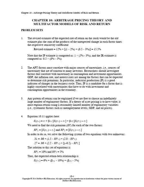
CHAPTER 10: ARBITRAGE PRICING THEORY ANDMULTIFACTOR MODELS OF RISK AND RETURN PROBLEM SETS1. The revised estimate of the expected rate of return on the stock would be the oldestimate plus the sum of the products of the unexpected change in each factor times the respective sensitivity coefficient:Revised estimate = 12% + [(1 × 2%) + (0.5 × 3%)] = 15.5%Note that the IP estimate is computed as: 1 × (5% - 3%), and the IR estimate iscomputed as: 0.5 × (8% - 5%).2. The APT factors must correlate with major sources of uncertainty, i.e., sources ofuncertainty that are of concern to many investors. Researchers should investigatefactors that correlate with uncertainty in consumption and investment opportunities.GDP, the inflation rate, and interest rates are among the factors that can be expected to determine risk premiums. In particular, industrial production (IP) is a goodindicator of changes in the business cycle. Thus, IP is a candidate for a factor that is highly correlated with uncertainties that have to do with investment andconsumption opportunities in the economy.3. Any pattern of returns can be explained if we are free to choose an indefinitelylarge number of explanatory factors. If a theory of asset pricing is to have value, itmust explain returns using a reasonably limited number of explanatory variables(i.e., systematic factors such as unemployment levels, GDP, and oil prices).4. Equation 10.11 applies here:E(r p) = r f + βP1 [E(r1 ) −r f ] + βP2 [E(r2 ) – r f]We need to find the risk premium (RP) for each of the two factors:RP1 = [E(r1 ) −r f] and RP2 = [E(r2 ) −r f]In order to do so, we solve the following system of two equations with two unknowns: .31 = .06 + (1.5 ×RP1 ) + (2.0 ×RP2 ).27 = .06 + (2.2 ×RP1 ) + [(–0.2) ×RP2 ]The solution to this set of equations isRP1 = 10% and RP2 = 5%Thus, the expected return-beta relationship isE(r P) = 6% + (βP1× 10%) + (βP2× 5%)5. The expected return for portfolio F equals the risk-free rate since its beta equals 0.For portfolio A, the ratio of risk premium to beta is (12 − 6)/1.2 = 5For portfolio E, the ratio is lower at (8 – 6)/0.6 = 3.33This implies that an arbitrage opportunity exists. For instance, you can create aportfolio G with beta equal to 0.6 (the same as E’s) by combining portfolio A and portfolio F in equal weights. The expected return and beta for portfolio G are then: E(r G) = (0.5 × 12%) + (0.5 × 6%) = 9%βG = (0.5 × 1.2) + (0.5 × 0%) = 0.6Comparing portfolio G to portfolio E, G has the same beta and higher return.Therefore, an arbitrage opportunity exists by buying portfolio G and selling anequal amount of portfolio E. The profit for this arbitrage will ber G – r E =[9% + (0.6 ×F)] − [8% + (0.6 ×F)] = 1%That is, 1% of the funds (long or short) in each portfolio.6. Substituting the portfolio returns and betas in the expected return-beta relationship,we obtain two equations with two unknowns, the risk-free rate (r f) and the factor risk premium (RP):12% = r f + (1.2 ×RP)9% = r f + (0.8 ×RP)Solving these equations, we obtainr f = 3% and RP = 7.5%7. a. Shorting an equally weighted portfolio of the ten negative-alpha stocks andinvesting the proceeds in an equally-weighted portfolio of the 10 positive-alpha stocks eliminates the market exposure and creates a zero-investmentportfolio. Denoting the systematic market factor as R M, the expected dollarreturn is (noting that the expectation of nonsystematic risk, e, is zero):$1,000,000 × [0.02 + (1.0 ×R M)] − $1,000,000 × [(–0.02) + (1.0 ×R M)]= $1,000,000 × 0.04 = $40,000The sensitivity of the payoff of this portfolio to the market factor is zerobecause the exposures of the positive alpha and negative alpha stocks cancelout. (Notice that the terms involving R M sum to zero.) Thus, the systematiccomponent of total risk is also zero. The variance of the analyst’s profit is notzero, however, since this portfolio is not well diversified.For n = 20 stocks (i.e., long 10 stocks and short 10 stocks) the investor willhave a $100,000 position (either long or short) in each stock. Net marketexposure is zero, but firm-specific risk has not been fully diversified. Thevariance of dollar returns from the positions in the 20 stocks is20 × [(100,000 × 0.30)2] = 18,000,000,000The standard deviation of dollar returns is $134,164.b. If n = 50 stocks (25 stocks long and 25 stocks short), the investor will have a$40,000 position in each stock, and the variance of dollar returns is50 × [(40,000 × 0.30)2] = 7,200,000,000The standard deviation of dollar returns is $84,853.Similarly, if n = 100 stocks (50 stocks long and 50 stocks short), the investorwill have a $20,000 position in each stock, and the variance of dollar returns is100 × [(20,000 × 0.30)2] = 3,600,000,000The standard deviation of dollar returns is $60,000.Notice that, when the number of stocks increases by a factor of 5 (i.e., from 20 to 100), standard deviation decreases by a factor of 5= 2.23607 (from$134,164 to $60,000).8. a. )(σσβσ2222e M +=88125)208.0(σ2222=+×=A50010)200.1(σ2222=+×=B97620)202.1(σ2222=+×=Cb. If there are an infinite number of assets with identical characteristics, then awell-diversified portfolio of each type will have only systematic risk since thenonsystematic risk will approach zero with large n. Each variance is simply β2 × market variance:222Well-diversified σ256Well-diversified σ400Well-diversified σ576A B C;;;The mean will equal that of the individual (identical) stocks.c. There is no arbitrage opportunity because the well-diversified portfolios allplot on the security market line (SML). Because they are fairly priced, there isno arbitrage.9. a. A long position in a portfolio (P) composed of portfolios A and B will offer anexpected return-beta trade-off lying on a straight line between points A and B.Therefore, we can choose weights such that βP = βC but with expected returnhigher than that of portfolio C. Hence, combining P with a short position in Cwill create an arbitrage portfolio with zero investment, zero beta, and positiverate of return.b. The argument in part (a) leads to the proposition that the coefficient of β2must be zero in order to preclude arbitrage opportunities.10. a. E(r) = 6% + (1.2 × 6%) + (0.5 × 8%) + (0.3 × 3%) = 18.1%b.Surprises in the macroeconomic factors will result in surprises in the return ofthe stock:Unexpected return from macro factors =[1.2 × (4% – 5%)] + [0.5 × (6% – 3%)] + [0.3 × (0% – 2%)] = –0.3%E(r) =18.1% − 0.3% = 17.8%11. The APT required (i.e., equilibrium) rate of return on the stock based on r f and thefactor betas isRequired E(r) = 6% + (1 × 6%) + (0.5 × 2%) + (0.75 × 4%) = 16% According to the equation for the return on the stock, the actually expected return on the stock is 15% (because the expected surprises on all factors are zero bydefinition). Because the actually expected return based on risk is less than theequilibrium return, we conclude that the stock is overpriced.12. The first two factors seem promising with respect to the likely impact on the firm’scost of capital. Both are macro factors that would elicit hedging demands acrossbroad sectors of investors. The third factor, while important to Pork Products, is a poor choice for a multifactor SML because the price of hogs is of minor importance to most investors and is therefore highly unlikely to be a priced risk factor. Betterchoices would focus on variables that investors in aggregate might find moreimportant to their welfare. Examples include: inflation uncertainty, short-terminterest-rate risk, energy price risk, or exchange rate risk. The important point here is that, in specifying a multifactor SML, we not confuse risk factors that are important toa particular investor with factors that are important to investors in general; only the latter are likely to command a risk premium in the capital markets.13. The formula is ()0.04 1.250.08 1.50.02.1717%E r =+×+×==14. If 4%f r = and based on the sensitivities to real GDP (0.75) and inflation (1.25),McCracken would calculate the expected return for the Orb Large Cap Fund to be:()0.040.750.08 1.250.02.040.0858.5% above the risk free rate E r =+×+×=+=Therefore, Kwon’s fundamental analysis estimate is congruent with McCracken’sAPT estimate. If we assume that both Kwon and McCracken’s estimates on the return of Orb’s Large Cap Fund are accurate, then no arbitrage profit is possible.15. In order to eliminate inflation, the following three equations must be solvedsimultaneously, where the GDP sensitivity will equal 1 in the first equation,inflation sensitivity will equal 0 in the second equation and the sum of the weights must equal 1 in the third equation.1.1.250.75 1.012.1.5 1.25 2.003.1wx wy wz wz wy wz wx wy wz ++=++=++=Here, x represents Orb’s High Growth Fund, y represents Large Cap Fund and z represents Utility Fund. Using algebraic manipulation will yield wx = wy = 1.6 and wz = -2.2.16. Since retirees living off a steady income would be hurt by inflation, this portfoliowould not be appropriate for them. Retirees would want a portfolio with a return positively correlated with inflation to preserve value, and less correlated with the variable growth of GDP. Thus, Stiles is wrong. McCracken is correct in that supply side macroeconomic policies are generally designed to increase output at aminimum of inflationary pressure. Increased output would mean higher GDP, which in turn would increase returns of a fund positively correlated with GDP.17. The maximum residual variance is tied to the number of securities (n ) in theportfolio because, as we increase the number of securities, we are more likely to encounter securities with larger residual variances. The starting point is todetermine the practical limit on the portfolio residual standard deviation, σ(e P ), that still qualifies as a well-diversified portfolio. A reasonable approach is to compareσ2(e P) to the market variance, or equivalently, to compare σ(e P) to the market standard deviation. Suppose we do not allow σ(e P) to exceed pσM, where p is a small decimal fraction, for example, 0.05; then, the smaller the value we choose for p, the more stringent our criterion for defining how diversified a well-diversified portfolio must be.Now construct a portfolio of n securities with weights w1, w2,…,w n, so that Σw i =1. The portfolio residual variance is σ2(e P) = Σw12σ2(e i)To meet our practical definition of sufficiently diversified, we require this residual variance to be less than (pσM)2. A sure and simple way to proceed is to assume the worst, that is, assume that the residual variance of each security is the highest possible value allowed under the assumptions of the problem: σ2(e i) = nσ2MIn that case σ2(e P) = Σw i2 nσM2Now apply the constraint: Σw i2 nσM2 ≤ (pσM)2This requires that: nΣw i2 ≤ p2Or, equivalently, that: Σw i2 ≤ p2/nA relatively easy way to generate a set of well-diversified portfolios is to use portfolio weights that follow a geometric progression, since the computations then become relatively straightforward. Choose w1 and a common factor q for the geometric progression such that q < 1. Therefore, the weight on each stock is a fraction q of the weight on the previous stock in the series. Then the sum of n terms is:Σw i= w1(1– q n)/(1– q) = 1or: w1 = (1– q)/(1– q n)The sum of the n squared weights is similarly obtained from w12 and a common geometric progression factor of q2. ThereforeΣw i2 = w12(1– q2n)/(1– q 2)Substituting for w1 from above, we obtainΣw i2 = [(1– q)2/(1– q n)2] × [(1– q2n)/(1– q 2)]For sufficient diversification, we choose q so that Σw i2 ≤ p2/nFor example, continue to assume that p = 0.05 and n = 1,000. If we chooseq = 0.9973, then we will satisfy the required condition. At this value for q w1 = 0.0029 and w n = 0.0029 × 0.99731,000In this case, w1 is about 15 times w n. Despite this significant departure from equal weighting, this portfolio is nevertheless well diversified. Any value of q between0.9973 and 1.0 results in a well-diversified portfolio. As q gets closer to 1, theportfolio approaches equal weighting.18. a. Assume a single-factor economy, with a factor risk premium E M and a (large)set of well-diversified portfolios with beta βP. Suppose we create a portfolio Zby allocating the portion w to portfolio P and (1 – w) to the market portfolioM. The rate of return on portfolio Z is:R Z = (w × R P) + [(1 – w) × R M]Portfolio Z is riskless if we choose w so that βZ = 0. This requires that:βZ = (w × βP) + [(1 – w) × 1] = 0 ⇒w = 1/(1 – βP) and (1 – w) = –βP/(1 – βP)Substitute this value for w in the expression for R Z:R Z = {[1/(1 – βP)] × R P} – {[βP/(1 – βP)] × R M}Since βZ = 0, then, in order to avoid arbitrage, R Z must be zero.This implies that: R P = βP × R MTaking expectations we have:E P = βP × E MThis is the SML for well-diversified portfolios.b. The same argument can be used to show that, in a three-factor model withfactor risk premiums E M, E1 and E2, in order to avoid arbitrage, we must have:E P = (βPM × E M) + (βP1 × E1) + (βP2 × E2)This is the SML for a three-factor economy.19. a. The Fama-French (FF) three-factor model holds that one of the factors drivingreturns is firm size. An index with returns highly correlated with firm size (i.e.,firm capitalization) that captures this factor is SMB (small minus big), thereturn for a portfolio of small stocks in excess of the return for a portfolio oflarge stocks. The returns for a small firm will be positively correlated withSMB. Moreover, the smaller the firm, the greater its residual from the othertwo factors, the market portfolio and the HML portfolio, which is the returnfor a portfolio of high book-to-market stocks in excess of the return for aportfolio of low book-to-market stocks. Hence, the ratio of the variance of thisresidual to the variance of the return on SMB will be larger and, together withthe higher correlation, results in a high beta on the SMB factor.b.This question appears to point to a flaw in the FF model. The model predictsthat firm size affects average returns so that, if two firms merge into a largerfirm, then the FF model predicts lower average returns for the merged firm.However, there seems to be no reason for the merged firm to underperformthe returns of the component companies, assuming that the component firmswere unrelated and that they will now be operated independently. We mighttherefore expect that the performance of the merged firm would be the sameas the performance of a portfolio of the originally independent firms, but theFF model predicts that the increased firm size will result in lower averagereturns. Therefore, the question revolves around the behavior of returns for aportfolio of small firms, compared to the return for larger firms that resultfrom merging those small firms into larger ones. Had past mergers of smallfirms into larger firms resulted, on average, in no change in the resultantlarger firms’ stock return characteristics (compared to the portfolio of stocksof the merged firms), the size factor in the FF model would have failed.Perhaps the reason the size factor seems to help explain stock returns is that,when small firms become large, the characteristics of their fortunes (andhence their stock returns) change in a significant way. Put differently, stocksof large firms that result from a merger of smaller firms appear empirically tobehave differently from portfolios of the smaller component firms.Specifically, the FF model predicts that the large firm will have a smaller riskpremium. Notice that this development is not necessarily a bad thing for thestockholders of the smaller firms that merge. The lower risk premium may bedue, in part, to the increase in value of the larger firm relative to the mergedfirms.CFA PROBLEMS1. a. This statement is incorrect. The CAPM requires a mean-variance efficientmarket portfolio, but APT does not.b.This statement is incorrect. The CAPM assumes normally distributed securityreturns, but APT does not.c. This statement is correct.2. b. Since portfolio X has β = 1.0, then X is the market portfolio and E(R M) =16%.Using E(R M ) = 16% and r f = 8%, the expected return for portfolio Y is notconsistent.3. d.4. c.5. d.6. c. Investors will take on as large a position as possible only if the mispricingopportunity is an arbitrage. Otherwise, considerations of risk anddiversification will limit the position they attempt to take in the mispricedsecurity.7. d.8. d.。