模形式理论
- 格式:pdf
- 大小:81.75 KB
- 文档页数:6
riemannzeta函数和模形式是数学领域中重要的概念,它们在数论、解析数论、自守形式等领域有着重要的作用。
本文将从理论和应用两个方面来介绍riemannzeta函数和模形式的基本概念、性质和相关的研究成果。
一、riemannzeta函数riemannzeta函数是数论中的重要函数,它被定义为复平面上的解析函数,其表达式为:\[ \zeta(s) = \sum_{n=1}^{\infty}\frac{1}{n^s} \]其中s是复数变量。
riemannzeta函数最初由黎曼在研究素数分布时引入,并在分析数论中占据着至关重要的地位。
riemannzeta函数具有许多重要的性质,比如在复平面上的解析性、黎曼函数方程等。
1.1 riemannzeta函数的解析性riemannzeta函数在复平面上的解析性是指它在定义域内是解析的,即对于复平面上的任意一点s,riemannzeta函数都有定义且在该点处有导数。
这一性质使得riemannzeta函数在复变函数论中占据着重要地位,也为研究riemannzeta函数的性质奠定了基础。
1.2 黎曼函数方程riemannzeta函数满足着著名的黎曼函数方程,即对于所有的s∈C\{1},都有:\[ \zeta(s) = 2^s\pi^{s-1}\sin(\frac{\pi s}{2})\Gamma(1-s)\zeta(1-s) \]这一函数方程表明了riemannzeta函数在复平面上的对称性,为研究riemannzeta函数的性质提供了极大的便利。
1.3 riemannzeta函数在数论中的应用riemannzeta函数在数论中有着许多重要的应用,其中最著名的莫过于黎曼假设。
黎曼假设是指所有非平凡的riemannzeta函数零点的实部都是1/2。
该假设在数论领域和素数分布领域有着深远的意义,然而至今尚未得到严格的证明。
二、模形式模形式是复变函数论中的一个重要概念,它起源于数论领域,随后发展成为一个独立的研究方向。
初中数学费马大定理的证明涉及到哪些数学分支和概念费马大定理的证明涉及到许多数学分支和概念,下面将详细介绍其中的一些主要数学分支和概念。
1. 代数几何:费马大定理的证明需要运用到代数几何的理论和方法。
代数几何是研究代数方程与几何图形之间的关系的数学分支。
在费马大定理的证明中,数学家们需要将方程a^n + b^n = c^n转化为几何图形,并通过几何的分析和研究来推导出结论。
代数几何的概念和工具在费马大定理的证明中发挥了重要的作用。
2. 数论:费马大定理是一个数论问题,涉及到了整数的性质和数学结构。
数论是研究整数及其性质的数学分支。
在费马大定理的证明中,数学家们需要研究方程a^n + b^n = c^n在整数域上的性质,探究其解的可能性。
数论的概念和理论为费马大定理的证明提供了基础和工具。
3. 模形式理论:费马大定理的证明涉及到了模形式理论的概念和方法。
模形式理论是研究特殊类型的复函数的数学分支,与费马大定理的证明有密切的联系。
数学家们利用模形式理论的工具和技巧,对费马大定理进行了深入的研究和探索,为证明提供了重要的思路和方法。
4. 椭圆曲线理论:费马大定理的证明涉及到了椭圆曲线理论的概念和技巧。
椭圆曲线理论是研究椭圆曲线及其性质的数学分支,与费马大定理的证明有重要的关联。
数学家们利用椭圆曲线理论的工具和方法,对费马大定理进行了深入的研究和分析,从而推动了证明的进展。
5. 调和分析:费马大定理的证明涉及到了调和分析的概念和技巧。
调和分析是研究周期函数的一种数学分支,与费马大定理的证明有一定的联系。
数学家们运用调和分析的方法和理论,对费马大定理进行了进一步的研究和分析,为证明提供了重要的工具和思路。
此外,费马大定理的证明还涉及到了其他数学分支和概念,如模论、解析数论、群论、模数论等。
数学家们通过运用多个数学分支的理论和方法,不断尝试和探索,才得以逐步接近费马大定理的证明目标。
总的来说,费马大定理的证明涉及到了代数几何、数论、模形式理论、椭圆曲线理论、调和分析等多个数学分支和概念。

1、概述Schur定理是裙论中的一个重要定理,它阐述了裙的中心有限指数的条件下,导裙是有限裙的结论。
本文将介绍Schur定理的定义、叙述及证明,从而深入理解该定理的内涵和应用。
2、Schur定理的定义在介绍Schur定理之前,我们先来了解一下裙的中心和导裙的概念。
(1)裙的中心:对于一个裙G,其中心Z(G)定义为所有满足对任意的g∈G都有gx=xg(其中x∈Z(G))的元素x的集合。
中心是裙中与所有元素都可交换的元素的集合。
(2)导裙:对于一个裙G,其导裙G'定义为由所有满足对任意的g,h∈G都有ghg^(-1)h^(-1)∈G'的元素组成的集合。
直观上讲,G'包含了G中“局部性质”的信息,它是G的一个重要的子裙。
有了上述概念的铺垫,我们可以正式介绍Schur定理。
Schur定理:如果一个裙的中心有限指数,则其导裙是有限裙。
3、Schur定理的叙述Schur定理的叙述是一个重要的结论,它指出了中心有限指数的裙的导裙是有限裙。
如果一个裙的中心的陪集数量是有限的,则其导裙是有限裙。
这一叙述对裙论的研究具有重要的指导意义,它为进一步研究裙的基本性质以及其结构提供了有力的支持。
4、Schur定理的证明Schur定理的证明涉及到一些裙论的基本知识和技巧,下面我们从几个重要步骤来梳理Schur定理的证明过程。
(1)引理1:设H是一个无限裙,N是H的一个有限指数的正规子裙,那么存在H的一个非平凡的正规子裙K,使得N∩K是K的有限指数的正规子裙。
(2)引理2:设Z(G)是一个有限指数的裙G的中心,那么对任意的a∈G,都有[C_G(a):C(a)∩Z(G)]<∞。
(3)引理3:设G是一个有限裙,那么G'的指数有界。
(4)证明:根据引理1和引理2,我们可以推出H的导裙G'是有限裙。
另外,根据引理3,我们可以得出G'的指数有界,从而可知G'是有限裙。
通过以上几步推理和引理,我们可以得出Schur定理的证明结论,即如果一个裙的中心有限指数,则其导裙是有限裙。

数学证明的实例分析在数学领域中,证明是非常重要的。
通过证明可以确定一个数学命题的真实性,解答各种问题,以及推进数学研究的发展。
本文将通过详细分析数学证明的实例,展示数学证明的重要性和基本方法。
实例一:费马大定理的证明费马大定理是数学史上最具盛名的问题之一,其原命题是:当整数n大于2时,关于x、y和z的方程x^n + y^n = z^n没有整数解。
曾经有数学家试图在几百年的时间里寻找证明,但直到1994年,安德鲁·怀尔斯(Andrew Wiles)才最终证明出来。
怀尔斯使用了模形式理论、代数几何和矩形陈理论等一系列高深的数学工具,通过构造性证明方法解决了费马大定理。
他首先通过建立两个椭圆曲线的等同性,从而证明了费马方程的奇特性质。
然后,他使用了模形式和Galois 表示等概念,最后在两个代数曲线的交点上应用了上面所说的矩形陈理论。
实例二:三角函数恒等式的证明三角函数恒等式是数学中常见的证明题型。
例如,我们可以考虑证明三角函数的和差公式:sin(a + b) = sin(a)cos(b) + cos(a)sin(b)。
为了证明这个恒等式,我们可以利用欧拉公式和三角函数的定义。
首先,我们将a和b表示成欧拉公式的形式,即a = α + β,b = γ + δ,其中α、β、γ、δ为实数。
然后,我们将欧拉公式代入到sin(a + b)的式子中,经过一系列化简和替换,最后可以得到sin(a + b) = sin(a)cos(b) + cos(a)sin(b),从而证明了和差公式的正确性。
实例三:数学归纳法的应用数学归纳法是一种重要的证明方法,可用于证明一类有序命题的正确性。
例如,我们可以利用数学归纳法证明1 + 2 + 3 + ... + n = n(n +1)/2。
首先,我们证明当n = 1时等式成立,即1 = 1(1 + 1)/2。
然后,我们假设当n = k时等式成立,即1 + 2 + 3 + ... + k = k(k + 1)/2。
费马四平方和定理费马四平方和定理费马四平方和定理,又称为费马猜想或费马大定理,是数学中的一个重要问题,它是由法国数学家皮埃尔·德·费马在17世纪提出的。
这个定理的内容是:任何一个大于2的自然数都可以表示成不超过4个自然数的平方和。
历史背景德·费马于1637年在他所写的《阿基米德原本》中提出了这个猜想。
他写道:“我有一种非常美妙的证明方法,但是这里没有足够的空间来容纳它。
”然而,直到他去世后,这个证明一直没有被找到。
随着时间的推移,越来越多的数学家尝试着证明这个猜想。
其中最著名的就是欧拉、拉格朗日、勒让德等人。
但他们都没有成功。
直到1908年,英国数学家哈代才发表了一篇论文,在其中给出了一个完整而严格的证明。
但是这份证明过于复杂,并且使用了20世纪初才发展起来的现代数学工具。
因此,在哈代之后,还有许多其他人尝试着给出更加简洁的证明。
其中最著名的就是苏联数学家维尔斯特拉斯在1975年给出的证明。
定理内容费马四平方和定理的内容非常简单,可以用一句话来概括:任何一个大于2的自然数都可以表示成不超过4个自然数的平方和。
换句话说,对于任意一个大于2的自然数n,都存在四个自然数a、b、c、d,使得:n = a² + b² + c² + d²这里a、b、c、d可以相等,也可以不相等。
证明方法费马四平方和定理的证明是非常复杂的。
以下是一种基于群论和模形式理论的较为简单的证明方法。
首先,假设存在某个大于2的自然数n无法表示成不超过4个自然数的平方和。
我们将这些无法表示成平方和的自然数称为“反例”。
接下来,我们考虑对每一个反例n构造一个模形式f(n)。
具体来说,我们定义:f(n) = Σ exp(2πi(a²+b²+c²+d²)n)其中Σ表示对所有满足a²+b²+c²+d²=n且a≤b≤c≤d的四元组(a,b,c,d)求和。
形式逻辑中的模型理论研究形式逻辑是一门研究推理和证明的学科,它以符号和形式化的语言为基础,通过建立逻辑系统和推理规则来分析推理的有效性和正确性。
而模型理论则是形式逻辑中的一个重要分支,它探讨的是逻辑语句在不同模型下的真值赋值情况,从而揭示了逻辑语句与现实世界之间的关系。
在形式逻辑中,一个模型是由一个非空集合和一组对集合中元素的赋值所组成的。
模型理论的研究对象是逻辑语句,通过为逻辑语句中的变量赋值,可以确定逻辑语句在不同模型下的真值。
模型理论的目标是研究逻辑语句的真值赋值规律,从而揭示逻辑语句的语义含义。
在模型理论中,一个重要的概念是满足关系。
满足关系是指在一个模型中,逻辑语句的真值赋值情况。
通过研究满足关系,可以确定逻辑语句的真值情况,从而判断逻辑语句的合法性和有效性。
满足关系可以用形式化的方式表示,例如使用真值表、真值函数等。
模型理论的研究方法主要包括语义方法和语法方法。
语义方法是通过研究逻辑语句在不同模型下的真值赋值情况,来揭示逻辑语句的语义含义。
语义方法的优点是直观、易于理解,但是缺点是计算复杂度较高。
语法方法是通过研究逻辑语句的形式和结构,来推导逻辑语句的真值赋值情况。
语法方法的优点是计算简单、效率高,但是缺点是对逻辑语句的形式和结构要求较高。
模型理论在形式逻辑中具有广泛的应用。
首先,模型理论可以用于验证逻辑系统的一致性和完备性。
通过构建逻辑系统的模型,可以验证逻辑系统中的公理和推理规则是否一致,并且可以确定逻辑系统是否完备。
其次,模型理论可以用于研究逻辑语句的语义含义。
通过研究逻辑语句在不同模型下的真值赋值情况,可以揭示逻辑语句的语义含义和逻辑结构。
最后,模型理论还可以用于研究逻辑语句的可满足性和有效性。
通过研究逻辑语句在不同模型下的真值赋值情况,可以确定逻辑语句是否可满足和有效。
总结而言,模型理论是形式逻辑中的一个重要分支,它研究的是逻辑语句在不同模型下的真值赋值情况。
通过研究满足关系和使用语义方法和语法方法,可以揭示逻辑语句的语义含义和逻辑结构。
费马引理的证明引言费马引理(Fermat’s Last Theorem)是数学史上一个著名的问题,由法国数学家皮埃尔·德·费马(Pierre de Fermat)在17世纪提出。
费马引理的内容是:对于任何大于2的正整数n,不存在满足以下方程的正整数解:a^n + b^n = c^n。
费马引理的证明是一个复杂且困难的数学问题,经历了几个世纪的努力才最终被证明。
本文将介绍费马引理的证明过程,并简要概述其中的关键思想和方法。
费马引理的证明过程费马引理的证明过程可以分为多个阶段,每个阶段都有其独特的思路和方法。
下面将逐步介绍这些阶段。
1. 初步尝试最早的证明尝试来自费马本人,他在边书中写下了“我有一个非常美妙的证明,但这里的空间太小,无法容纳。
”这句话成为了数学史上的经典之谜,也为后来的数学家们提供了巨大的启发。
2. 特殊情况的证明费马引理在特殊情况下的证明比较容易,比如当n=3时,费马引理可以被直接证明。
这个证明是由英国数学家安德鲁·怀尔斯(Andrew Wiles)在1994年完成的,他使用了复杂的代数几何工具和模形式理论。
3. 椭圆曲线方法费马引理的证明过程中,椭圆曲线方法起到了至关重要的作用。
这个方法是由法国数学家雅克·迪利涅(Jacques de Dines)和德国数学家海因里希·韦伊斯特拉斯(Heinrich Weber)提出的。
椭圆曲线方法的关键思想是将费马引理转化为椭圆曲线上的一个问题。
通过研究椭圆曲线的性质和结构,数学家们可以得到关于费马引理的有用信息。
4. 贝兹等式的应用费马引理的证明还需要用到贝兹等式(Bezout’s identity)。
贝兹等式是代数几何中的一个基本定理,它描述了两个多项式的最大公因式与它们的系数之间的关系。
通过应用贝兹等式,数学家们可以得到费马引理的一些限制条件,从而进一步缩小证明的范围。
5. 基于模形式的证明最后,费马引理的证明使用了模形式(Modular Forms)理论。

《费马大定理》教学设计教学目标:知识与技能1、了解费马大定理的产生和证明过程;2、了解类比推理是从特殊到特殊的推理;3、正确认识合情推理在数学中的重要作用;4、养成从小开始认真观察事物、分析问题、发现事物之间的联系的良好个性品质,善于发现问题,探求新知识。
过程与方法通过学习费马大定理,认识类比推理这一种合情推理的基本方法,并把它用于对问题的发现中去。
情感态度与价值观认识数学在日常生产生活中的重要作用,培养学生学数学,用数学,完善数学的正确数学意识。
教学重点:能利用类比进行简单的推理。
教学难点:由费马大定理总结出,类比推理,并用类比进行推理,做出猜想。
教具准备:与教材内容相关的资料。
课时安排:1课时教学过程:一、费马大定理1、业余数学家之王费马(Fermat,1601—1665),法国数学家,他非常喜欢数学,常常利用业余时间研究高深的数学问题,结果取得了很大的成就,被人称为“业余数学家之王”,费马凭借丰富的想象力和深刻的洞察力,提出一系列重要的数学猜想。
2、费马小猜想1640年,费尔马在研究质数性质时,发现了一个有趣的现象:当n=1时,22n+1=221+1=5;当n=2时,22n+1=222+1=17;当n=3时,22n+1=223+1=257;当n=4时,22n+1=224+1=65537;猜测:只要n是自然数, 22n+1一定是质数1732年,欧拉进行了否定3、费马小定理如果P是一个质数,那么对于任何自然数n,n P-n一定能够被P整除.这个猜想已证明是正确的,这个猜想被称为“费马小定理”,利用费马小定理,是目前最有效的鉴定质数的方法4、费马大定理1637年前后,费马在读古希腊丢番图的《算术》这本书的靠近问题8的页边处记下这样一个结论(现在的写法):同时又写下一个附加的评注:“对于该命题,我确信已发现一种奇妙的证明,可惜这里的空白太小,写不下”5、费马大定理产生的历史性背景费尔马大定理,启源于两千多年前,挑战人类三个多世纪,多次震惊全世界,耗尽人类最杰出大脑的精力,也让千千万万业余者痴迷。

一、政策制定的理论模型什么是模型模型是现实世界某些方面的简单化呈现。
它可以是:--一个实体的呈现(如飞机模型)--一种图示(如流程图)--一种公式(如S=v〃t)--一段文字表述的概念(如“桌子是由一个面板及其下面的四条木棍支撑而成的一种家具”)什么是政策分析模型政策分析模型是公共政策的一种的简单化呈现。
通常以概念的方式出现(概念模型)政策分析模型有何作用1.简化我们对公共政策的思维2.指出政策议题的重要方面3.通过将注意力在政治生活的重要特征,有助于我们进行有效的沟通4.提出公共政策中不重要的因素,加深我们的了解5.解释公共政策的要素,预测其影响人们很少能选定那些一劳永逸、自成一体、所有人都能领会的政策。
政策分析的目的不是产生某种一锤定音的政策建议,而是要帮助人们对现实可能性和期望之间有逐渐一致的认识,产生一种新型的社会相互关系与“社会心理”模式。
——米切尔〃怀特主要的政策制定理论模型1.精英模型2.团体模型3.多元模型4.完全理性模型5.有限理性模型6.渐进模型7.混合扫描模型8. 系统模型从完全理性的假设(最优)→有限理性(满意)→非理性的假设(合理)(一)精英模型代表人物及著作:1970年托马斯.戴伊(Thom as Dye)和哈蒙.齐格勒(Harmo n Zeigler)在《民主的嘲讽》中总结了前辈的精英理论基本内容:精英决策模型是将公共政策看成是反映占统治地位的精英(elite)们的价值和偏好的一种决策理论。
从政治精英到社会精英从圣西门到拉斯韦尔基本要点:社会可以划分为拥有权力的少数人,以及不拥有权力的多数人。
只有少数人才有权为社会分配价值,而群众则不能决定公共政策少数管理者并不代表多数被管理者。
精英大多从社会经济地位较高的上层阶级中选拔非精英往精英地位的流动必须缓慢而持续,以维持社会稳定并避免革命发生。
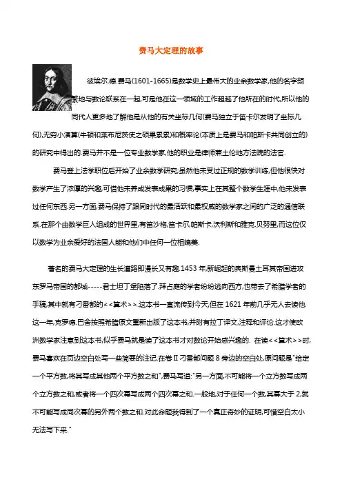
费马大定理的故事彼埃尔.德.费马(1601-1665)是数学史上最伟大的业余数学家,他的名字频繁地与数论联系在一起,可是他在这一领域的工作超越了他所在的时代,所以他的同代人更多地了解他是从他的有关坐标几何(费马独立于笛卡尔发明了坐标几何),无穷小演算(牛顿和莱布尼茨使之硕果累累)和概率论(本质上是费马和帕斯卡共同创立的)的研究中得出的.费马并不是一位专业数学家,他的职业是律师兼土伦地方法院的法官.费马登上法学职位后开始了业余数学研究;虽然他未受过正规的数学训练,但他很快对数学产生了浓厚的兴趣,可惜他未养成发表成果的习惯,事实上在其整个数学生涯中,他未发表过任何东西.另一方面,费马保持了跟同时代的最活跃和最权威的数学家之间的广泛的通信联系.在那个由数学巨人组成的世界里,有笛沙格,笛卡尔,帕斯卡,沃利斯和雅克.贝努里,而这位仅以数学为业余爱好的法国人能和他们中任何一位相媲美.著名的费马大定理的生长道路即漫长又有趣.1453年,新崛起的奥斯曼土耳其帝国进攻东罗马帝国的都城-----君士坦丁堡陷落了.拜占庭的学者纷纷逃向西方,也带去了希腊学者的手稿,其中就有刁番都的<<算术>>.这本书一直流传到今天,但在1621年前几乎无人去读他.这一年,克罗德.巴舍按照希腊原文重新出版了这本书,并附有拉丁译文,注释和评论.这才使欧洲数学家注意到这本书,似乎费马就是读了这本书才对数论开始感兴趣的. 在读<<算术>>时,费马喜欢在页边空白处写一些简要的注记.在卷II刁番都问题8旁边的空白处,原问题是"给定一个平方数,将其写成其他两个平方数之和",费马写道:"另一方面,不可能将一个立方数写成两个立方数之和,或者将一个四次幂写成两个四次幂之和.一般地,对于任何一个数,其幂大于2,就不可能写成同次幂的另外两个数之和.对此命题我得到了一个真正奇妙的证明,可惜空白太小无法写下来."用代数术语表达,刁番都问题是想求出方程:x2+y2=z2的有理数解,这已经由古希腊数学家欧几里德得到:x=2mn,y=m2-n2,z=m2+n2而费马在页边的注解断言,若n是大于2的自然数,则方程x n+y n=z n不存在有理数解.这就是我们今天称为费马大定理的由来.尽管在普通人的心目中,相信费马真的找到了一个奇妙的证明,但他毕竟是一个动人的故事,17世纪的一位业余数学爱好者证明了一个结果,他使得其后350年间的数学家起来为之奋斗了,然而却劳而无功.他的问题是如此简明,因而这个故事更富有感染力.而且永远存在费马是正确的可能性. 从费马的另一处注解中,数学史家发现了费马唯一具体的对于n=4的情形做的证明,在这个证明中,费马发明了一种"无穷递降法",他利用了整数边直角三角形的面积不可能是平方数的结论,假设方程:x4+y4=z4有一组有理解,令a=x4,b=2x2z2,c=z4+x4,d=y2xz.反复利用熟知的恒等式:(s+t)2=s2+2st+t2 得到:a2+b2=(z4-x4)2+4x4z4=z8-2x4z4+x8+4x4z4=(z4+x4)2=c2.并且有:ab/2=y42x2z2=(y2xz)2=d2于是,a2+b2=c2,并且ab/2=d2.但是这已经证明是不可能的,因此假定n=4时有解是错误的. 对于n=3的情形,后来的欧拉在1753年用了一种有缺陷的方法证明了这个命题.他使用了一种"新数",即形如a+b√-3的数系,这个数系在许多方面与整数有相似之处,两者都构成一个数环.但他并不具备整数的全部性质,欧拉证明中用到的最要紧的性质是唯一因子分解定理,对于a+b√-3数系,这个定理碰巧也成立,所以欧拉的结论是正确的.但是换成别的形式比如a+b√-5,则唯一因子分解定理就不成立了.关于对于什么样的数系唯一因子分解定理成立的理论叫做示性类理论.接着,1825年,20岁的狄利赫莱和70岁的勒让德同时证明了n=5.1832年,法国杰出的女数学家索非.热尔曼证明:若p是奇素数并使得2p+1也是素数,则费马大定理成立.1839年,拉梅证明了n=7.取得突破性进展的是德国数学家E.库莫尔,1847年,他证明了对于小于100的除了37,59和67这三个所谓非正则素数以外,费马大定理成立.在这一证明过程中,库莫尔的最重要贡献不在于费马大定理本身,而是发明了一种全新的概念-----理想数,这是一种特别有用的涉及范围极广的概念,他将引出一个更一般的概念------理想,以及整个新的数学分支-----理想论,后者的基本原理现在已经成为大学一般数学系学生的必修课.1983年,29岁的德国数学家G.法尔廷斯证明了一个结论:对于每一个大于2的指数n,费马方程x n+y n=z n至多有有限多个解.这一证明使他赢得了1986年的菲尔兹奖.他把存在无穷多个解的可能性降低到最多只可能有有限多个解,这确实是一个巨大的成就.但是,费马大定理被彻底征服的途径一定会使涉及到这一领域的所有前人出乎意外,最后的攻坚路线跟费马本人,欧拉和库莫尔等人的完全不同,他是现代数学诸多分支(椭圆曲线论,模形式理论,伽罗华表示理论,等等)综合发挥作用的结果.其中最重要的武器是椭圆曲线和模形式理论.在50年代,日本数学家谷山丰和志村五郎提出一个猜想:有理数域上的每条椭圆曲线都有同构的模形式存在(今天我们一般称之为谷山-志村猜想).所谓椭圆曲线是由椭圆积分衍化而来的,他是如下形式的三次曲线:y2=Ax3+Bx2+Cx+D 而模形式是解析数论中研究的一种函数的运算(模函数是满足某种线性变换的复变函数,而摸形式是处处全纯的摸函数运算,全纯是指函数的摸是有限的).而通过相似的格,可以将椭圆曲线与摸形式联系在一起.从60年代开始,有人将费马方程x n+y n=z n和形如y2=x(x+A)(x+B)(1)的椭圆曲线相联系,最初的着眼点是利用跟费马大定理有关的结论来证明与椭圆曲线有关的结论.1984年秋,G.弗赖在两者的联系方面迈出了关键性的一步,他参加了在德国黑森州奥波沃尔法赫小城举行的一次数学讨论会上演说中提出:假定费马大定理不成立,即存在一组非零整数a,b,c使得a n+b n=c n (n>2),那么用这组解构造出的形如(1)的椭圆曲线(在(1)中令A=a n , B=-b n ,现在称这类椭圆曲线为弗赖曲线),不可能是摸形式.而这与谷山-志村猜想矛盾.如果弗赖的结论和谷山-志村猜想都得到证明是正确的,根据反证法的逻辑可知,"假定费马大定理不成立"是错的,因而导出费马大定理正确.可惜弗赖本人未能证明自己的论断;但是在1986年,K.里贝特按照美国数学家J.P.赛尔的思想证明了弗赖的论断.于是,证明费马大定理的工作归结为去证明谷山-志村猜想.当时的数学家们普遍认为,要证明谷山-志村猜想还是很遥远的事情,但是,年轻的英国数学家安德鲁.怀尔斯对这种看法不以为然,他立即集中全部精力去证明这个猜想.经过7年的艰苦奋斗,怀尔斯于1993年6月在英国剑桥大学牛顿数学科学研究所举行的数学讨论会上,报告了他对如下结论的证明:对于有理数域上的一大类椭圆曲线(用专业术语称为半稳定的椭圆曲线),谷山-志村猜想成立.由于弗赖曲线恰好属于半稳定的椭圆曲线的范围,因此费马大定理自然地成为怀尔斯的推论.据称怀尔斯的证明长达200页.按照数学界的习惯,他的证明在得到确认之前,必须经过其他有关数学家的详细审查,尽管当时许多人相信怀尔斯的证明是经得起推敲的.好事多磨,事情并未就此了结.有关怀尔斯的证明中存在漏洞的传闻不胫而走.1993年12月4日,怀尔斯给他的同行们发出了一封电子邮件,承认他的证明中确有漏洞.数学家对待证明的态度是十分严肃的,不容半点含糊.1994年10月25日,美国俄亥俄州立大学的教授K.鲁宾以电子邮件的形式向数学界的朋友发出了谨慎而乐观的消息:"今天早上,有两篇论文已经发表,他们是:"椭圆模曲线和费马大定理",作者是安德鲁.怀尔斯;"某些赫克代数的环论性质",作者是R.泰勒和安德鲁.怀尔斯.第一篇是一篇长文,...他宣布了费马大定理的一个证明,而这个证明中关键的一步依赖于第二篇短文...."1995年7月号的"美国数学会通告"上发表了G.法尔廷斯的文章,题为"R.泰勒和A.怀尔斯对费马大定理的证明".他开宗明义,以肯定的语调宣称:"在本文题目中所提到的猜想于1994年9月终于被完整地证明了."至此,人们相信那个搅扰了数学家300多年的著名的猜想真正成为了一条定理!虽然费马大定理已经被证明了,但是也引起我们深入的哲学思考,怀尔斯是用归纳法来证明谷山-志村猜想的,即对于椭圆曲线的E-序列,对应着模形式的M-序列,并且应用了数学中高深的群论思想.那么我们要想,当年费马写在刁番都<<算术>>的空白处的"奇妙的证明"到底存在吗?无独有偶,我国的一位学者蒋春喧在怀尔斯之前就已经用初等数学的方法证明了费马大定理,并且得到了我国数论专家乐茂华和美国科学家桑蒂利的支持,想必不会是没有根据的错误论证.我们假设是正确的,那么这是否就是费马本人想到的那种"奇妙的证明"呢?对于这个问题,我们只能关注事态的发展,拭目以待最后的结果了.我至今还未找到我国学者蒋春喧的有关费马大定理的简单证明.等我找到之后会写完本篇文章,如果那位网友能帮助我找到,我将不胜感激,谢谢.获奖和评论1995-96年度数学沃尔夫(Wolf)奖由怀尔斯和朗兰兹(Robert P. Langlands)分享,于1996年3月24日在耶路撒冷由以色列总统魏兹曼颁发,奖金十万美元.沃尔夫基金会称,怀尔斯得奖是“由于对数论及相关领域的壮观贡献,由于在若干基本猜想上得到的巨大进展,由于解决了费尔马大定理". 美国数学会的报道说, 怀尔斯引入深刻的奇异的方法, 对于数论中一些长期未决的基本问题的解决作出了巨大的贡献.例如, BSD猜想, 伊瓦萨瓦(Iwasawa)理论主猜想, 和谷山丰-志村五郎(Taniyama-Shimura)猜想. 他的工作的顶峰是对令人称颂的费尔马大定理的证明, 此定理塑造了过去两个世纪大多数论的形态. 朗兰兹是60岁的著名数学家,他的“朗兰兹猜想"影响深远,博大精深.沃尔夫数学奖的历届得主都是极负盛名的数学家,如盖尔丰德,西格尔,韦伊,嘉当,陈省身,小平邦彦等. 该奖是国际上极有影响的大奖,由沃尔夫捐款在1978年设立. 也有化学,医药,农业,和艺术奖.(沃尔夫原居德国,一战前移居古巴,1961年起任古巴驻以色列大使,后留居以色列.与德国专门为费马大定理而设的沃尔夫斯克尔奖无关.).怀尔斯获美国“国家科学院奖”被宣布是奖励“他对费马大定理的证明,这是他发明了一种美丽的战略,证明了志村五郎-谷山丰猜想的一大部分才完成的;也是奖励他在追求自已的思想实现的过程中所表现出的勇气和技巧力量". 此奖是在1988年为纪念美国数学会一百周年设立的, 奖金五千美元,奖给近十年内发表的杰出数学研究. 以前的得主是朗兰兹(1989)和麦克费尔逊(1993).美国数学会在上述得奖报道中,刊登了怀尔斯过去的导师剑桥大学的蔻茨(J. Coates)的评论文章. 文章说: 怀尔斯在牛津大学毕业后, 于1974-75学年度到剑桥."他的天才很快被斯文哪尔敦--戴尔(Swinnerton-Dyer)注意到. 他因管理剑桥大学太忙, 不能作怀尔斯的研究生导师,对这我很高兴. 结果当怀尔斯1975夏开始科研时,我非常幸运地得以能指导他的数学研究第一步"."我们最后得以证明平行于伊瓦撒瓦的结果",证明了BSD猜想的秩零特殊情况."我很快认识到他具有两个显著的数学禀赋,我相信这在他以后的全部数学生涯中都起了关键的作用.第一,他优先于一切地要去证明困难的具体定理,而不愿去作优美的无所不包的猜想. 第二, 他有惊人的能力去吸收大量的极高深极抽象的机制, 并在脚踏实地的问题中贯彻直到得出巨大的成果".到1980年代中期, 怀尔斯"对于伊瓦撒瓦理论主猜想和关于希尔波特模形式的伽罗华表示的研究贡献, 已经使他成为过去150年以来对代数数论作出渊深贡献的极少数优秀数学家之一. 但是, 正象我们现在所知道的, 他并没有躺在这些桂冠上休息, 而从1986年夏他又一直默默地工作着, 朝向一个更伟大的目标.""过去35年的代数数论和算术代数几何,大多被猜想所统治, 而少有肯定的定理. 这并不是要贬毁期间证明的许多优美的定理, 只是要指出太常有的情况: 面对着那些大叠大排的猜想, 这些肯定的结果显得太拘谨, 而那些猜想的证明要留作代数数论的长期目标(例如, 椭圆曲线的BSD猜想, 或者阿庭关于他的非阿贝尔L-函数的全纯猜想). 安德鲁·怀尔斯的工作是对这种研究模式的绝妙解毒剂,也是我们时代的最响亮的警示: 我们是能够期望最终解开数论中那些最深奥的神谜的."怀尔斯的生平安德鲁.怀尔斯(Andrew Wiles)1953年4月11日生于英国剑桥.(所以他1993年6月宣布证明时,刚过四十岁生日两个多月.) 1971年入牛津大学莫顿(Merton)学院学习, 1974年获该校学士学位. 同年入剑桥大学柯雷尔(Clare)学院学习, 1980年获该校博士学位. 1977至1980年,是柯雷尔学院的“青年研究会员”和哈佛大学的“本杰明·裴尔斯助教授”. 1981年是波恩的“理论数学专门研究院”访问教授,此年稍后,为美国普林斯顿的“高等研究所”研究员. 1982年成为普林斯顿大学教授,该年春是奥赛的巴黎大学访问教授. 作为古根海姆特别研究员,他1985--86年是科学高级研究所(IHES)和高级师范学校(ENS)的访问教授. 1988至90年,是牛津大学皇家学会研究教授. 1994年,他取得现在的普林斯顿大学欧根·黑金斯数学教授职位. 怀尔斯于1989年被选为在伦敦的皇家学会研究员. 1995年获瑞典皇家科学院的数学韶克奖. 同年获费尔马奖,由保罗萨巴提尔大学和马特拉马克尼空间颁发. 1996年获沃尔夫奖,和[美国]国家科学院奖.费马大定理的玩笑很多年以前,一个叫作费马的同志在法院工作,他总是抱这么一本书--丢番图写的《算术》第三册,正如很多年以后一个叫做Jonny的人总是抱着一本Windows NT 宝典一样。
deta函数Dedekind eta函数(也称为Dedekind eta函数)是一个重要的数学函数,它在数论和代数学中都有重要应用。
在数论中,它与模形式和模曲线密切相关。
Dedekind eta函数是一个称为模函数的特殊函数,其定义如下:对于任何复数τ,Dedekind eta函数的值为:η(τ) = q^(1/24) ∏_(n=1)^∞(1 - q^n)其中q = e^(2πiτ)是模形式理论中的模函数。
该函数被证明是一个权重为1/2的模形式,并在理论物理中的玻色-菲尔米混合系统中有广泛应用。
Dedekind eta函数具有许多重要的性质,其中包括以下内容:1. Dedekind eta函数是一个奇函数,即η(-τ) = -η(τ)。
2. Dedekind eta函数的第一项系数是q^(1/24),这使得它在τ= i处为零。
3. Dedekind eta函数具有满足乘法公式的性质,即:η(τ+ 1) = e^(πi/12)η(τ)4. Dedekind eta函数还具有另一个满足乘法公式的版本,称为三重乘积公式:η(τ) = q^(1/24) ∏_(n=1)^∞(1 -q^n) = 2^(1/4)∙3^(1/24)∙Π_(n=1)^∞[1 + (-1)^n∙2^(2n-1)/(1-2^n)∙3^(n-1/2)∙q^(n-1/2)]其中Π表示乘积,q=e^(2πiτ)。
5. Dedekind eta函数具有模同余性质,即:η(τ+ m + nτ') = e^(-πimn/τ')∙e^(-2πin(τ+τ'))∙η(τ)其中m、n为任意整数,τ、τ'为任意复数。
总之,Dedekind eta函数是一个在数学中具有广泛应用的特殊函数,其定义和性质都具有深刻而重要的数学意义。
数论中的模形式与L函数数论是数学的一个重要分支,研究整数及其性质。
数论中的模形式与L函数是两个重要的概念,它们在数论研究中起着关键的作用。
一、模形式在数论中,模形式是一种特殊的函数,具有一些特定的性质。
它是从复平面到复数域的映射,可以看作是一种“函数”的推广。
模形式由一些特定的变换性质来定义,并且在数论中具有重要的应用。
数论中的模形式主要分为两类:尖点和非尖点的模形式。
尖点的模形式是指在上半平面中解析且满足一些特定的变换性质的函数。
非尖点的模形式是指在上半平面中解析但不满足特定变换性质的函数。
模形式的研究可以追溯到19世纪末20世纪初,由德国数学家狄德金和魏尔斯特拉斯首次引入。
随后,一系列的研究成果使得模形式在数论中得到了广泛的应用,尤其是与L函数的关系。
二、L函数L函数是数论中的一个重要函数,用于研究数论中的各种问题。
L 函数的定义相对较复杂,但其核心思想是将数论中的问题转化为复平面上的函数性质。
在数论中,L函数以欧拉和黎曼的名字命名。
它包含了数论中的一些重要信息,例如数论常数、素数分布等。
L函数在数论研究中起着重要的作用,它与模形式之间存在一种紧密的联系。
模形式与L函数之间的联系是数论中的一个重要研究领域,称为模形式的L函数理论。
通过分析模形式的L函数,可以得到关于模形式性质的重要结论,同时也可以推导出关于数论问题的结果。
三、模形式与L函数的应用模形式与L函数在数论中有广泛的应用。
它们的研究成果为解决众多数论问题提供了重要的方法和工具。
例如,在费马猜想的证明中,模形式与L函数的理论发挥了重要作用。
费马猜想是一个著名的数论问题,涉及到勾股数的存在性问题。
通过研究模形式的L函数,数学家们得到了关于费马猜想的一些重要结论。
此外,模形式与L函数在密码学、编码理论等领域也有着广泛的应用。
它们的理论不仅在数论中具有重要意义,同时也对其他领域的研究起到了推动作用。
综上所述,数论中的模形式与L函数是两个重要的概念,它们在数论研究中发挥着关键的作用。
数论的模形式
数论中的模形式是指一类特殊的函数,它们具有特定的变换性质。
模形式在数论与代数几何之间建立了一座桥梁,它们有广泛的应用于数论、代数几何、物理学等领域。
模形式的定义可以从多个角度进行,其中一种常见的定义是通过研究椭圆函数得到的。
椭圆函数是一类具有周期性和交换性质的函数,它们在复平面上具有特定的形式。
通过对椭圆函数进行变换,可以得到模形式。
模形式的一个重要性质是它们具有积分表示形式,即可以通过积分来表示模形式的值。
这种表示形式使得研究模形式的性质变得更加方便。
同时,模形式还具有一系列的变换性质,比如变换公式、边界条件等,这些性质使得模形式在数论中有着广泛的应用。
模形式在数论中的应用非常丰富,其中一个重要的应用是与椭圆曲线的研究相联系。
椭圆曲线是一类特殊的代数曲线,其上的点构成了一个具有特定性质的集合。
通过研究椭圆曲线的点,可以得到与模形式相关的算术结构,从而揭示了数论中一系列深刻的结果,比如费马大定理、椭圆曲线的模意义、球面上的点的等式等。
总之,数论中的模形式是一类具有特定变换性质的函数,它们在数论与代数几何之间建立了桥梁,并在数论中有着广泛的应用。
数学中的模形式在数学领域中,模形式是一种非常重要且广泛研究的数学对象。
它们具有许多精彩的特性和应用,涉及到数论、代数几何和理论物理等众多领域。
本文将简要介绍模形式的基本概念和相关性质,并探讨一些模形式在数学和其他学科中的应用。
一、模形式的概念模形式是一种特殊的解析函数,具有一定的对称性和变换性质。
它们最早由德国数学家费尔德(Karl Theodor Wilhelm Weierstrass)在19世纪提出,并由法国数学家庞加莱(Henri Poincaré)在20世纪初进一步发展和研究。
模形式的定义涉及到复变函数理论和群论等多个数学分支。
在数学中,最常见的模形式是椭圆模形式,它们是特殊类型的模形式。
椭圆模形式通常涉及到椭圆曲线、倍数关系和模空间等概念,是代数几何和数论的重要对象。
二、模形式的性质模形式具有一系列优良的性质,这些性质为它们在数学研究中的广泛应用提供了基础。
1. 模变换性质:模形式在特定的线性分数变换下具有不变性。
这种不变性是模形式表现出来的对称性,反映了复平面及其上的离散群对模形式的作用。
2. 级形式:模形式的级是指它在离散子群下的不变性。
级越高的模形式具有更多的约束条件和特殊性质,研究级较高的模形式是数论和代数几何中的重要方向之一。
3. Fourier展开:模形式可以通过Fourier级数展开,这种展开形式方便了模形式的计算和研究。
Fourier展开还揭示了模形式的周期性结构和与数论问题的关联。
4. 模空间:模空间是所有模形式构成的空间。
模空间的研究在代数几何和数论中具有重要意义,它们是模形式的几何化,提供了一种几何理解模形式的方法。
三、模形式的应用模形式在数学和其他学科中有着广泛的应用。
以下列举几个例子:1. 数论:模形式与数论之间有着紧密的联系,特别是在椭圆曲线与模形式的关系中。
模形式的理论为解决一些数论难题提供了强有力的工具和方法。
2. 物理学:模形式在理论物理学中也有着一定的应用,特别是在弦论和量子场论等领域。
高数费马定理费马定理,又称费马大定理,是数学史上的一颗明珠。
它的内容是:对于任何大于2的整数n,关于x、y、z的方程xn + yn = zn在整数域上没有解。
这个定理是由法国数学家费马于17世纪提出的,但一直未能找到完整的证明,直到1994年,英国数学家安德鲁·怀尔斯发表了一篇论文,给出了费马定理的证明。
下面我们就来了解一下费马定理的背景和证明过程。
费马定理的背景可以追溯到古希腊时代,当时的数学家们对于某些特殊的整数方程有所研究。
然而,直到费马的时代,这个问题才被提出并引起了广泛的关注。
费马本人在给朋友写信时提到了这个定理,并声称自己已经找到了简洁的证明,但他没有公开发表这个证明。
这引起了无数数学家的兴趣和挑战,他们试图寻找费马所谓的证明,但徒劳无功。
费马定理的证明是一个复杂而漫长的过程。
怀尔斯的证明主要基于椭圆曲线和模形式的理论,这些概念在数学中是相当高级和抽象的。
怀尔斯通过构造一种特殊的椭圆曲线来证明费马定理,这个曲线与方程xn + yn = zn有密切的关系。
通过研究这个椭圆曲线的性质,怀尔斯最终得出了结论:对于任何大于2的整数n,方程xn + yn = zn在整数域上没有解。
怀尔斯的证明过程非常复杂,充满了高深的数学理论和技巧。
他运用了模形式的理论,这是一种复变函数论的分支,用于研究椭圆曲线的性质。
通过这一理论的运用,怀尔斯成功地证明了费马定理,并填补了数学史上的一个重要空白。
费马定理的证明不仅仅是一个数学问题,它还涉及到数学思维的深化和数学理论的发展。
怀尔斯的证明不仅解决了费马定理这个具体问题,也为后人提供了许多新的思路和方法。
他的证明在数学界引起了巨大的反响,被誉为“20世纪最重要的数学结果之一”。
费马定理的证明不仅仅对数学有重要意义,它还对其他领域产生了广泛的影响。
例如,在密码学中,椭圆曲线密码是一种基于椭圆曲线的加密算法,它的安全性与费马定理有密切的关系。
怀尔斯的证明为椭圆曲线密码的发展提供了理论支持,使得它成为了现代密码学中最重要的算法之一。
数学费马大定理的证明思路费马大定理,又称费马猜想,是指对于任何大于2的整数n,不存在满足a^n + b^n = c^n的正整数解a、b、c。
这一问题是数学领域中的开放问题,在数学史上占据重要地位。
最初由法国数学家费马在1637年提出并在其笔记中写下:“我已有较好的证法,但此证法太大,无法容纳于此处,我恐怕再也无法找到与此相同美妙的证法了。
”然而,费马从未公布过其证明,使得数学界为之沉迷,直到1994年才由英国数学家安德鲁·怀尔斯给出了完整的证明。
费马大定理证明的思路主要分为以下几个步骤:1. 引入数学工具首先,为了证明费马大定理,需要引入一些数学工具和理论。
其中最重要的是代数、数论和解析几何等领域的数学知识。
特别是椭圆曲线和模形式的理论,它们被证明是证明费马大定理的关键。
2. 将费马大定理转化为等价问题由于费马大定理的难度相对较大,数学家们普遍采用转化为等价问题的方式来求解。
具体而言,将费马大定理转化为断言,即假设存在某个正整数n>2,使得a^n + b^n = c^n有正整数解。
然后,通过推理和逻辑推导,去掉其中的矛盾和不可能性,从而证明费马大定理。
3. 使用费马导数定理为了证明费马大定理,需要运用费马导数定理。
费马导数定理是费马在研究曲线的极值问题时发现的重要性质。
该定理指出,如果函数在某一点处取极值,且该点是函数图像的平坦点(即导数为零),那么该点也必然是该函数图像的极值点。
通过使用费马导数定理,可以对方程进行推理和变换,从而获得更多有用的信息。
4. 利用模形式理论安德鲁·怀尔斯在证明费马大定理时,运用了模形式理论。
模形式是一种数论和解析几何的重要数学对象,它具有深厚的数学基础和广泛的应用领域。
通过研究椭圆曲线和模形式的性质,怀尔斯得到了一组方程,这些方程揭示了费马大定理存在椭圆曲线的一种特殊情况。
5. 排除特殊情况在证明费马大定理时,需要考虑各种可能的特殊情况,以确保得出的结论适用于所有情况。
CHAPTER IINTRODUCTIONIntroduction to the First(1992)EditionThis book is in three sections.First,we describe in detail an algorithm based on modular symbols for computing modular elliptic curves:that is,one-dimensional factors of the Jacobian of the modular curve X0(N),which are attached to certain cusp forms for the congruence subgroupΓ0(N).In the second section,various algorithms for studying the arithmetic of elliptic curves(defined over the rationals)are described.These are for the most part not new, but they have not all appeared in book form,and it seemed appropriate to include them here. Lastly,we report on the results obtained when the modular symbols algorithm was carried out for all N≤1000.In a comprehensive set of tables we give details of the curves found, together with all isogenous curves(5113curves in all,in2463isogeny classes1).Specifically, we give for each curve the rank and generators for the points of infinite order,the number of torsion points,the regulator,the traces of Frobenius for primes less than100,and the leading coefficient of the L-series at s=1;we also give the reduction data(Kodaira symbols,and local constants)for all primes of bad reduction,and information about isogenies.For N≤200these curves can be found in the well-known tables usually referred to as “Antwerp IV”[2],as computed by Tingley[67],who in turn extended earlier tables of curves found by systematic search;our calculations agree with that list in all281cases.For values of N in the range200<N≤320Tingley computed the modular curves attached to newforms forΓ0(N)only when there was no known curve of conductor N corresponding to the newform: these appear in his thesis[67]but are unpublished.As in[2],the curves E we list for each N have the following properties.(1)They have conductor N,as determined by Tate’s algorithm[65].(2)The coefficients given are those of a global minimal model for E,and these coefficients(or,more precisely,the c4and c6invariants)agree with the numerical values obtained from the modular calculation to several decimal places:in most cases,depending on the accuracy obtained—see below—differing by no more than10−30.(3)Their traces of Frobenius agree with those of the modular curves for all primes p<1000.We have also investigated,for each curve,certain numbers related to the Birch–Swinnerton-Dyer conjecture.Let f(z)be a newform forΓ0(N)with rational Fourier coefficients,and E the elliptic curve defined over Q attached to f.The value of L(f,1)is a rational multiple of a period of f,and may be computed easily using modular symbols(see[37]and Section2.8below).We have computed this rational number in each case,andfind that it is always consistent with the Birch–Swinnerton-Dyer conjecture for E.More specifically,letΩ0(f)be the least positive real period of F andΩ(f)=2Ω0(f)orΩ0(f)according as the period lattice of f is or is not rectangular.Then wefind that L(f,1)/Ω(f)=0if(and only if)the Mordell-Weil group E(Q) 1In thefirst edition,these numbers were given as5089and2447respectively,as the curves of conductor702 were inadvertently omitted.12I.INTRODUCTIONhas positive rank,and when E(Q)isfinite wefind in each case thatL(f,1)/Ω(f)= p|N c p·|E(Q)|−2·Swith S∈N(in fact S=1in all but four cases:S=4in three cases and S=9in one case). This is consistent with the Birch–Swinnerton-Dyer conjecture if the Tate–Shafarevich group X isfinite of order S.(Here c p is the local index[E(Q p):E0(Q p)];see[58,p.362].)When L(f,1)=0,we compute the sign w of the functional equation for L(f,s),and verify that w=+1if and only if the curve has even rank.More precisely,we also compute the value of L(r)(f,1),where r is the rank,the regulator R,and the quotientS=L(r)(f,1)r!Ω(f) (c p)R|E(Q)tors|2.In all but the four cases mentioned above wefind that S=1to within the accuracy of the computation.Our algorithm uses modular symbols to compute the1-homology ofΓ0(N)\H∗where H∗is the extended upper half-plane{z∈C:Im(z)>0}∪{∞}∪Q.While similar in some respects to Tingley’s original algorithm described in[67],it also uses ideas from[37]together with some new ideas which will be described in detail below.One important advantage of our method, compared with Tingley’s,is that we do not need to consider explicitly the exact geometric shape of a fundamental region for the action ofΓ0(N)on H∗:this means that highly composite N can be dealt with in exactly the same way as,say,prime N.Of course,for prime N there are other methods,such as that of Mestre[43],which are probably faster in that case,though not apparently yielding the values of the“Birch–Swinnerton-Dyer numbers”L(f,1)/Ω(f).There is also a strong similarity between the algorithms described here and those developed by the author in his investigation of cusp forms of weight two over imaginary quadraticfields[12], [13],[15].A variant of this algorithm has also been used successfully to study modular forms forΓ0(N)with quadratic character,thus answering some questions raised by Pinch(see[48] or[49])concerning elliptic curves of everywhere good reduction over real quadraticfields.See [14]for details of this,and for a generalization toΓ1(N):one couldfind cusp forms of weight two with arbitrary character using this extension of the modular symbol method,though at present it has only been implemented for quadratic characters,as described in[14].It is not our intention in this book to discuss the theory of modular forms in any detail, though we will summarize the facts that we need,and give references to suitable texts.The theoretical construction and properties of the modular elliptic curves will also be excluded, except for a brief summary.Likewise,we will assume that the reader has some knowledge of the theory of elliptic curves,such as can be obtained from one of the growing number of excellent books on the subject.Instead we will be concentrating on computational aspects, and hope thus to complement other,more theoretical,treatments.In Chapter2we describe the various steps in the modular symbol algorithm in detail.At each step we give the theoretical foundations of the method used,with proofs or references to the literature.Included here are some remarks on our implementation of the algorithms,which might be useful to those wishing to write their own programs.At the end of this stage we have equations for the curves,together with certain other data for the associated cusp form:Hecke eigenvalues,sign of the functional equation,and the ratio L(f,1)/Ω(f).Following Chapter2,we give some worked examples to illustrate the various methods.In Chapter3we describe the algorithms we used to study the elliptic curves we found using modular symbols,including thefinding of all curves isogenous to those in the original list.INTRODUCTION TO THE SECOND(1996)EDITION3 These algorithms are more generally applicable to arbitrary elliptic curves over Q,although we do not consider questions which might arise with curves having bad reduction at very large primes.(For example,we do not consider how to factorize the discriminant in order tofind the bad primes,as in all cases in the tables this is trivially achieved by trial division).Here we compute minimal equations,local reduction types,rank and torsion,generators for the Mordell–Weil group,the regulator,and traces of Frobenius.This includes all the information published in the earlier Antwerp IV tables.Thefinal calculations,relating to the Birch–Swin-nerton-Dyer conjecture,are also described here;these combine values obtained from the cusp forms(specifically,the leading coefficient of the expansion of the L-series at s=1,and the real period)with the regulator and local factors obtained directly from the curves.Thus we can compute in each case the conjectural value S of the order of X,the Tate–Shafarevich group.Finally,in Chapter4we discuss the results of the computations for N≤1000,and introduce the tables which follow.All the computer programs used were written in Algol68(amounting to over10000lines of code in all)and run on the ICL3980computer at the South West Universities Regional Computing Centre at Bath,U.K..The author would like to express his thanks to the staffof SWURCC for their friendly help and cooperation,and also to Richard Pinch for the use of his Algol68multiple-length arithmetic package.At present,our programs are not easily portable, mainly because of the choice of Algol68as programming language,which is not very generally available.However we are currently working on a new version of the programs,written in a standard version of the object-oriented language C++,which would be easily portable.The elliptic curve algorithms themselves are currently(1991)available more readily,in a number of computer packages.2In particular,the package apecs,written in Maple and available free via anonymousfile transfer from Ian Connell of McGill University,will compute all the data we have included for each curve.(A slightly limited version of apecs,known as upecs,runs under UBASIC on MS-DOS machines).There are also elliptic curve functions available for Mathematica(Silverman’s Elliptic Curve Calculator)and in the PARI/GP package.These packages are all in the process of rapid development.An earlier version of Chapter2of this book,with the tables,has been fairly widely circulated, and several people have pointed out errors which somehow crept in to the original tables.We have made every effort to eliminate typographical errors in the tables,which were typeset directly from datafiles produced by the programs which did the calculations.Where possible, the data for each curve has been checked independently using other programs.Amongst those who have spotted earlier errors or have helped with checking,I would like to mention Richard Pinch,Harvey Rose,Ian Connell,Noam Elkies,and Wah Keung Chan;obviously there may still be some incorrect entries,but these remain solely my responsibility.Introduction to the Second(1996)EditionSince thefirst edition of this book appeared in1992,some significant advances have been made in the algorithms described and in their implementation.The second edition contains an account of these advances,as well as correcting many errors and omissions in the original text and tables.We give here a summary of the more substantial changes to the text and tables.Of course,the most significant theoretical advance of the last four years is the proof by Wiles,Taylor–Wiles and others of most cases of the Shimura–Taniyama–Weil conjecture,which almost makes the word“modular”in the title of this book redundant.However,the only effect the new results have on this work are to guarantee that every elliptic curve defined over the rationals and of conductor less than1000is isomorphic to one of those in our Table1.2See the end of the introduction for more on obtaining these packages.4I.INTRODUCTIONChapter2.Section2.1has been completely rewritten and expanded to give a much more coherent,self-contained,and(we hope)correct account of the theoretical background to the modular symbol method.The text here is based closely on some unpublished lecture notes of the author for a series of lectures he gave in Bordeaux in1995at the meeting“´Etat de la Recherche en Algorithmique Arithm´e tique”organized by the Soci´e t´e Math´e matique de France.In Section2.4,we give a self-contained treatment of the method of Heilbronn matrices for computing Hecke operators,similar to the treatment by Merel in[42],as this now forms part of our implementation.In Section2.10,we give a new method of computing periods of cusp forms,as described in[18],which is as efficient as the“indirect”method;this largely makes the indirect method redundant,but we still include it in Section2.11.Also in Section2.11,we include some tricks and shortcuts which we have developed as we pushed the computations to higher levels, which can greatly reduce the computation time needed tofind equations for the curves of conductor N,at the expense of not necessarily knowing which is the so-called“strong Weil”curve in its isogeny class.Section2.14has been rewritten to take into account the results of Edixhoven on the Manin constant(see[21]),which imply that the values of c4and c6which we compute for each curve are known a priori to be integral.This means that the values we compute are guaranteed to be correct,and eliminates the uncertainty previously existing as to whether the curves we obtain by rounding the computed values are the modular elliptic curves they are supposed to be.Section2.15is entirely new:we show how to compute the degree of the modular parametriza-tion mapϕ:X0(N)→E for a modular elliptic curve of conductor N,using our version(see [17])of a method of Zagier[69].This method is easy to implement within the modular sym-bol framework,and we have added it to our programs,so that we now compute the degree automatically for each curve wefind.The appendix to Chapter2,containing worked examples,now includes the Heilbronn matrix method,and also illustrates some of the tricks mentioned in Section2.11.Implementation changes.The implementations of all the algorithms described here have been completely rewritten in C++,to be easily portable.We use the GNU compiler gcc for this.For multiprecision arithmetic we use either the GNU package libg++or the package LiDIA.For solving the systems of linear equations giving the relations between M-symbols, we use sparse matrix routines which not only reduce memory requirements,but also speed up that part of the computations considerably.These routines were written by L.Figueiredo specifically for his work on imaginary quadraticfields(see[24])which in turn built on the author’s work in[12]and[13].Chapter3.In Section3.1we give simpler formulae for recovering the Weierstrass coefficients of a curve from the invariants c4and c6;this enables us to simplify the Kraus–Laska–Connell algorithm slightly.In Section3.4we give a slightly improved formula for the global canonical height,and include this as a separate algorithm.Section3.5now contains references to other bounds between the naive and canonical heights,and other methods for the infinite descent step,but without details.The main changes in this chapter are to Section3.6on two-descent algorithms.On the one hand,we give a better explanation of the theoretical basis for these algorithms,making the account more self-contained(though we do not include all proofs).We have also moved the discussion on testing homogeneous spaces for local and global solubility forward,as this is common to the two main algorithms(general two-descent and two-descent via2-isogeny).On the other hand,several parts of the algorithm have been subject to major improvements over the last few years,thanks to collaboration with P.Serf,S.Siksek and N.P.Smart,and theseINTRODUCTION TO THE SECOND(1996)EDITION5 are now included.Notable here are the syzygy sieve in the search for quartics,the systematic use of group structure in the2-isogeny case,and the use of quadratic sieving in searching for rational points on homogeneous spaces.We also simplify the test for equivalence of quartics and the process of recovering rational points on the curve from points on the homogeneous spaces.Many of these improvements are from the author’s paper[20],which contains some proofs omitted here.Implementation changes.As with the modular symbol algorithms,we have rewritten all the elliptic curve algorithms in C++.In the case of the program tofind isogenies,which is very sensitive to the precision used,we have written an independent implementation in PARI/GP; using this we have a check on the isogeny computations which gave the isogenous curves listed in Table1.(The standard precision version of this program,while much faster,does miss several of the isogenies,for reasons given in Section3.8.)Versions of our algorithms will shortly become generally available in two forms.First,the package LiDIA(a library of C++classes for computational number theory,developed by the LiDIA group at the Universit¨a t des Saarlandes in Germany)will include them in a coming release.Secondly,the package Magma is also in the process of implementing the algorithms.In addition to these packages and those mentioned in the original Introduction,we should also mention the package Simath,developed by H.G.Zimmer’s research group in Saarbr¨u cken, which also has a large collection of very efficient elliptic curve algorithms.See the end of this Introduction for how to obtain more information on these packages.Chapter4and Tables.The two main changes in the tables are to include all the data for N=702in Tables1–4and include the new Table5giving the degree of the modular parametrization for each strong Weil curve.The omission of level702in thefirst edition is hard to explain;in our original implementation andfile structure,it was not possible to distinguish between a level which had run successfully,but with no rational newforms found,and a level which had not yet run.The original runs were done as batch jobs on a remote mainframe computer,with manual record-keeping to keep track of which levels had run successfully.Our current implementation is much more robust in this respect.We are grateful to Henri Cohen whofirst discovered this error on comparing our data with his own tables(of modular forms of varying weight and level,computed by him together with Skoruppa and Zagier).The omission was also noted by Jacques Basmaji of Essen,who recomputed Table3independently.The new implementationfinds the newforms at each level in a consistent order.In the original runs,the order in which the newforms were found changed as the program developed. Unfortunately,we did not recompute the earlier levels with thefinal version of the program before publishing thefirst edition of the tables,and the identifying letter for each newform given in the tables has now become standard.Hence our current implementation reorders the newforms during output to agree with the order as originally published(this is necessary for 147levels in all,the largest being450).Also concerning the order and naming of the curves:the convention we normally use is that in each isogeny class thefirst curve is the strong Weil curve whose period lattice is exactly that of the corresponding newform forΓ0(N),such as11A1for example.In precisely one case,an error caused thefirst curve listed in class990H to be not the strong Weil curve but a curve isogenous to it.The strong Weil curve in this class is in fact990H3and not990H1.In the notation of Section2.11,the correct values of l+and m+to obtain the strong Weil curve 990H3are13and8,but for some reason we had used the value m+=24which leads to the 3-isogenous curve990H1.In Table1,the other corrections are:N=160has the Antwerp codes corrected,and916B1 has a spurious indication of a non-existent3-isogeny removed.In Table2,we include the generators for the curves of conductor702and positive rank,and6I.INTRODUCTIONagain correct the Antwerp code for curve160A1.We also give the generator of427C1correctly as(−3,1)rather than(−3,0)as previously,and for990H we give the generator(−35,97)of the strong Weil curve990H3rather than a generator of990H1as before.In Table3,as well as inserting the data for N=702,we correct the eigenvalues for N=100 which had been given incorrectly.In Table4,we insert the data for N=702and also for600E–600I which had been omitted by mistake.Moreover,for N=990we give the data for990H3instead of990H1as before,as this is the strong Weil curve(the only difference being thatΩhas been multiplied by3and R divided by3).Extension of the ing our new implementation of the algorithms of Chapter2,we have extended the computations of all modular elliptic curves up to conductor5077(chosen as the smallest conductor of a curve of rank3).We have also computed in each case the other data tabulated here for conductors up to1000.For reasons of space,we cannot print extended versions of the tables:as there are17598newforms(or isogeny classes)and a total of31586 curves up to5077,this would have made this book approximately six times as thick as it is at present!Instead,the data for curves whose conductors lie in the range from1001to5077(and beyond, as they become available)may be obtained by anonymousfile transfer from the author’s web site at /personal/jec/ftp/data/INDEX.html Finally,many thanks to those who have told me of misprints and other errors in the First Edition,including J.Basmaji,G.Bailey,B.Brock,F.Calegari,J.W.S.Cassels,T.Kagawa, B.Kaskel,P.Serf,S.Siksek,and N.Smart.Apologies to any whose names have been omitted. Extra thanks are also due to Nigel Smart,who read a draft of Chapter3of the Second Edition, and made useful suggestions.web and ftp sitesMore information on the packages mentioned above,and in most cases the packages them-selves,can be obtained from the following web and ftp sites.Apart from Magma they are all free.apecs(for Maple):ftp://math.mcgill.ca/pub/apecsElliptic Curve Calculator(for Mathematica):ftp:///dist/EllipticCurve LiDIA:http://www-jb.cs.uni-sb.de/LiDIAMagma:.au:8000/comp/magma mwrank:ftp:///pub/cremona/progsPARI/GP:ftp://megrez.math.u-bordeaux.fr/pub/pariSimath:http://emmy.math.uni-sb.de/~simathupecs(for UBASIC):ftp://math.mcgill.ca/pub/upecsLinks to all of these can be found at the following place,which will be updated./personal/jec/packages.html。