HST Luminosity Functions of the Globular Clusters M10, M22, and M55. A comparison with othe
- 格式:pdf
- 大小:772.51 KB
- 文档页数:14

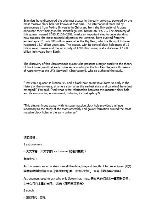
风云卫星数据和产品应用手册第1章概述1.1 FY-3A卫星概况风云三号A气象卫星(简称FY-3A)是我国的第二代太阳同步极轨气象卫星。
风云三号气象卫星将实现全球、全天候、多光谱、三维、定量对地观测。
风云三号星发射总质量为2450kg,发射尺寸:4.38m×2m×2m,卫星长期功耗1130W。
卫星本体由服务舱、推进舱与有效载荷舱组成。
服务舱采用中心承力筒和隔板结构,主要安装电源、测控、数管及姿轨控分系统的部件和设备、推进舱采用中心承筒和隔板结构,主要安装推进系统设备以及蓄电池组和放电调节器。
有效载荷舱隔板和构架结构,主要安装探测仪器的探测头部,舱内主要安装探测仪器的电子设备等。
风云三号A卫星有十一台遥感探测仪器。
遥感数据通过两个实时传输信道(HRPT和MPT)和一个延时传输信道(DPT)进行传输。
风云三号A卫星设计寿命为3年。
1.2 主要技术指标1.2.1 卫星轨道⑴轨道类型:近极地太阳同步轨道⑵轨道标称高度:831公里⑶轨道倾角:98.81°⑷入轨精度:半长轴偏差: |Δa|≤5公里轨道倾角偏差:|Δi|≤0.1°轨道偏心率≤0.003⑸标称轨道回归周期为5.79天⑹轨道保持偏心率:≤0.00013⑺交点地方时漂移:2年小于15分钟⑻卫星发射窗口:降交点地方时10:051.2.2 卫星姿态⑴姿态稳定方式:三轴稳定⑵三轴指向精度:≤0.3°⑶三轴测量精度:≤0.05°⑷三轴姿态稳定度:≤4×10⁻³ °/s1.2.3 太阳帆板对日定向跟踪1.2.4 星上记时⑴记时方式:J2000日计数和日毫秒计数⑵记时单位:1毫秒⑶时间精度(星地总精度):小于20毫秒1.2.5 遥感探测仪器性能指标1.2.5.1 可见光红外扫描辐射计(VIRR)(1)通道数、各通道波段范围、灵敏度见表1-1。
(2)空间分辨率:星下点分辨率1.1Km(3)扫描范围:±55.4°(4)扫描器转速:6线/秒(5)每条扫描线采样点数:2048(6)MTF≥0.3(7)通道配准:飞行方向/扫描方向星下点配准精度<0.5个像元(8)扫描抖动:<0.8个IFOV(9)通道信号衰减:<15%/2年(10)量化等级:10比特(11)定标精度:可见光和近红外通道:CH1、2、7、8、9 7%(反射率)CH6、10 10%(反射率)红外通道:1k(270k)。
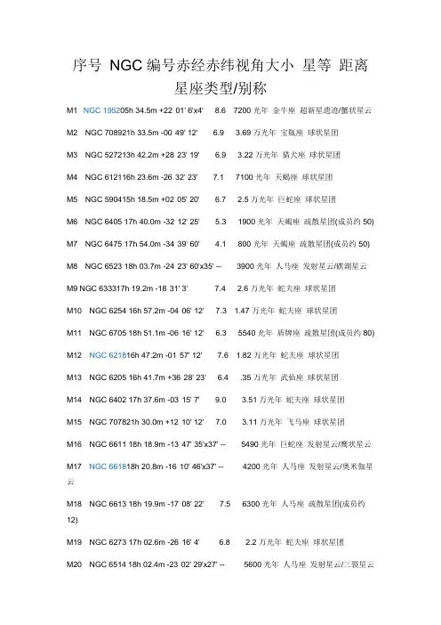
序号NGC编号赤经赤纬视角大小星等距离星座类型/别称M1 NGC 195205h 34.5m +22°01' 6'x4' 8.6 7200光年金牛座超新星遗迹/蟹状星云M2 NGC 708921h 33.5m -00°49' 12' 6.9 3.69万光年宝瓶座球状星团M3 NGC 527213h 42.2m +28°23' 19' 6.9 3.22万光年猎犬座球状星团M4 NGC 612116h 23.6m -26°32' 23' 7.1 7100光年天蝎座球状星团M5 NGC 590415h 18.5m +02°05' 20' 6.7 2.5万光年巨蛇座球状星团M6 NGC 6405 17h 40.0m -32°12' 25' 5.3 1900光年天蝎座疏散星团(成员约50) M7 NGC 6475 17h 54.0m -34°39' 60' 4.1 800光年天蝎座疏散星团(成员约50) M8 NGC 6523 18h 03.7m -24°23' 60'x35' -- 3900光年人马座发射星云/礁湖星云M9 NGC 633317h 19.2m -18°31' 3' 7.4 2.6万光年蛇夫座球状星团M10 NGC 6254 16h 57.2m -04°06' 12' 7.3 1.47万光年蛇夫座球状星团M11 NGC 6705 18h 51.1m -06°16' 12' 6.3 5540光年盾牌座疏散星团(成员约80) M12 NGC 621816h 47.2m -01°57' 12' 7.6 1.82万光年蛇夫座球状星团M13 NGC 6205 16h 41.7m +36°28' 23' 6.4 .35万光年武仙座球状星团M14 NGC 6402 17h 37.6m -03°15' 7' 9.0 3.51万光年蛇夫座球状星团M15 NGC 707821h 30.0m +12°10' 12' 7.0 3.11万光年飞马座球状星团M16 NGC 6611 18h 18.9m -13°47' 35'x37' -- 5490光年巨蛇座发射星云/鹰状星云M17 NGC 661818h 20.8m -16°10' 46'x37' -- 4200光年人马座发射星云/奥米伽星云M18 NGC 6613 18h 19.9m -17°08' 22' 7.5 6300光年人马座疏散星团(成员约12)M19 NGC 6273 17h 02.6m -26°16' 4' 6.8 2.2万光年蛇夫座球状星团M20 NGC 6514 18h 02.4m -23°02' 29'x27' -- 5600光年人马座发射星云/三裂星云40)M22 NGC 665618h 36.4m -23°54' 18' 6.3 1.03万光年人马座球状星团M23 NGC 649417h 56.9m -19°01' 25' 6.9 4500光年人马座疏散星团(成员约120)M24 NGC 660318h 18.4m -18°25' 4.5' 4.5 1.6万光年人马座星团及星云M25 NGC 472518h 31.6m -19°14' 40' 6.5 2000光年人马座疏散星团(成员约50)M26 NGC 669418h 45.2m -09°24' 9' 9.3 4900光年盾牌座疏散星团(成员约20)M27 NGC 685319h 59.6m +22°43' 8'x4' 7.6 820光年狐狸座行星状星云/哑铃星云M28 NGC 662618h 24.6m -24°52' 5' 6.8 1.5万光年人马座球状星团M29 NGC 6913 20h 24.0m +38°31' 12' 7.1 3000光年天鹅座疏散星团(成员约20)M30 NGC 709921h 40.4m -23°11' 6' 6.4 4.1万光年魔羯座球状星团M31 NGC 224 00h 42.7m +41°16' 180'x63' 4.4 230万光年仙女座星系/仙女座大星云M32 NGC 221 00h 42.7m +40°52' 8'x6' 9.2 230万光年仙女座椭圆星系M33 NGC 598 01h 33.8m +30°39' 62'x39' 6.3 250万光年三角座旋涡星系M34 NGC 1039 20h 42.0m +42°47' 30' 5.5 1390光年英仙座疏散星团(成员约60)M35 NGC 2168 06h 08.8m +24°20' 40' 5.3 2600光年双子座疏散星团(成员约120)M36 NGC 1960 05h 36.3m +34°08' 17' 6.3 4110光年御夫座疏散星团(成员约50)约200)M38 NGC 1912 05h 28.7m +35°50' 18' 7.4 4610光年御夫座疏散星团(成员约100)M39 NGC 7092 21h 32.3m +48°26' 30' 5.2 864光年天鹅座疏散星团(成员约20)M40 -- 12h 22.4m +58°05' -- 8.0 -- 大熊座双星M41 NGC 2287 06h 47.0m -20°46' 30' 5.0 2500光年大犬座疏散星团(成员约50)M42 NGC 1976 05h 35.3m -05°23' 66'x60' -- 1500光年猎户座发射星云/猎户大星云M43 NGC 1982 05h 35.5m -05°16' 20'x15' -- 1500光年猎户座发射星云M44 NGC 2632 08h 40.0m +20°00' 90' 3.7 520光年巨蟹座疏散星团/蜂巢星团M45 -- 03h 47.5m +24°07' 120'x120' 1.4 410光年金牛座疏散星团/昴星团M46 NGC 2437 07h 41.8m -14°49' 24' 6.0 6000光年船尾座疏散星团(成员约150)M47 NGC 2422 07h 36.7m -14°29' 25' 4.5 1800光年船尾座疏散星团(成员约50)M48 NGC 2548 08h 13.8m -05°48' 30' 5.3 1500光年长蛇座疏散星团(成员约80)M49 NGC 4472 12h 29.8m +08°00' 9'x7' 9.3 5900光年室女座椭圆星系M50 NGC 2323 07h 03.0m -08°21' 16' 6.9 2600光年麒麟座疏散星团(成员约100)M51 NGC 5194 13h 29.4m +47°12' 11'x8' 9.0 2100光年猎犬座旋涡星系M52 NGC 7654 23h 24.2m +61°36' 12' 7.3 3800光年仙后座疏散星团(成员约120)M53 NGC 5024 13h 12.9m +18°10' 14' 8.3 5.64万光年后发座球状星团M54 NGC 6715 18h 55.1m -30°28' 2' 7.1 4.9万光年人马座球状星团M55 NGC 6809 19h 40.0m -30°57' 10' 4.4 1.9万光年人马座球状星团M56 NGC 6779 19h 16.6m +30°11' 5' 9.6 3.3万光年天琴座球状星团M57 NGC 6720 18h 53.6m +33°02' 1.4'x1' 9.3 2300光年天琴座行星状星云/环状星云M58 NGC 4579 12h 37.7m +11°49' 3'x2' 9.2 4100万光年室女座旋涡星系M59 NGC 4621 12h 42.0m +11°39' 3'x2' 9.8 4100万光年室女座椭圆星系M60 NGC 4649 12h 43.7m +11°33' 7'x6' 9.8 5900万光年室女座椭圆星系M61 NGC 4303 12h 21.9m +04°28' 7'x2' 6.6 4100万光年室女座旋涡星系M62 NGC 6266 17h 01.2m -30°07' 6' 7.8 2.06万光年蛇夫座球状星团M63 NGC 5055 13h 15.8m +42°02' 12'x8' 9.3 2400万光年猎犬座旋涡星系M64 NGC 4826 12h 56.7m +21°41' 9'x5' 9.4 1500万光年后发座旋涡星系M65 NGC 3623 11h 18.9m +13°06' 8'x2' 9.9 2700万光年狮子座旋涡星系M66 NGC 3627 11h 20.3m +13°00' 9'x4' 9.7 2700万光年狮子座旋涡星系M67 NGC 2682 08h 51.3m +11°48' 17' 6.9 2710光年巨蟹座疏散星团(成员约80)M68 NGC 4590 12h 39.5m -26°45' 10' 8.7 3.14万光年长蛇座球状星团M69 NGC 6637 18h 31.4m -32°21' 3' 7.5 2.4万光年人马座球状星团M70 NGC 6681 18h 43.2m -32°17' 3' 7.5 6.5万光年人马座球状星团M71 NGC 6838 19h 53.7m +18°47' 6' 7.9 1.33万光年天箭座球状星团M72 NGC 6981 20h 53.5m -12°32' 2' 8.6 5.9万光年宝瓶座球状星团M73 NGC 6994 20h 59.0m -12°38' 3' 8.9 -- 宝瓶座疏散星团(不定) M74 NGC 628 01h 36.7m +15°47' 10'x10' 9.8 3700万光年双鱼座旋涡星系M75 NGC 6864 20h 06.1m -21°55' 2' 8.6 7.8万光年人马座球状星团M76 NGC 651 01h 42.4m +51°34' 2.6'x1.5' 12.2 8000光年英仙座行星状星云M77 NGC 1068 02h 42.7m -00°01' 7'x6' 9.5 4700万光年鲸鱼座塞佛特星系M78 NGC 2068 05h 46.7m +00°04' 8'x6' -- 1600光年猎户座反射星团M79 NGC 1904 05h 24.2m +24°31' 4' 8.1 4.3万光年天兔座球状星团M80 NGC 6093 16h 17.1m +22°59' 4' 6.8 3.7万光年天蟹座球状星团星系M82 NGC 3034 09h 56.2m +69°42' 11x5' 9.3 1400万光年大熊座不规则星系M83 NGC 5236 13h 37.7m -29°32' 11'x10' 8.2 1600万光年长蛇座棒旋星系M84 NGC 4374 12h 25.1m +12°53' 5'x5' 10.3 4100万光年室女座椭圆星系M85 NGC 4382 12h 25.4m +18°11' 7'x4' 9.9 4100万光年后发座椭圆星系M86 NGC 4406 12h 26.2m +12°57' 8'x7' 9.9 2000万光年室女座椭圆星系M87 NGC 4486 12h 30.8m +12°23' 7'x7' 9.6 5900万光年室女座椭圆星系M88 NGC 4501 12h 32.0m +14°25' 8'x4' 10 4100万光年后发座旋涡星系M89 NGC 4552 12h 35.7m +12°33' 2'x2' 9.5 4100万光年室女座椭圆星系M90 NGC 4569 12h 36.8m +13°10' 8'x2' 10.0 4100万光年室女座旋涡星系M91 NGC 4548 12h 35.4m +14°30' 3'x2' 11.6 4100万光年后发座棒旋星系M92 NGC 6341 17h 17.1m +43°08' 12' 6.9 2.55万光年武仙座球状星团M93 NGC 2447 07h 44.6m -23°53' 25' 6.0 3600光年船尾座疏散星团(成员约60)星系M95 NGC 3351 10h 44.0m +11°42' 6'x6' 10.4 2900万光年狮子座棒旋星系M96 NGC 3368 10h 46.8m +11°49' 7'x4' 9.9 2900万光年狮子座旋涡星系M97 NGC 3587 11h 14.9m +55°01' 3.4'x3.3' 12.0 1800光年大熊座行星状星云/夜枭星云M98 NGC 4192 12h 13.8m +14°54' 10'x3' 10.5 3600万光年后发座旋涡星系M99 NGC 4254 12h 18.8m +14°25' 5'x5' 10.2 4 100万光年后发座旋涡星系M100 NGC 4321 12h 22.9m +15°49' 7'x6' 9.9 4100万光年后发座旋涡星系M101 NGC 5457 14h 03.2m +54°21' 27'x26' 8.2 1900万光年大熊座旋涡星系M102 NGC 5866 15h 06.5m +55°46' 5'x2' 11.0 -- 天龙座旋涡星系M103 NGC 581 01h 33.1m +60°42' 7' 7.4 7990光年仙后座疏散星团(成员约30)M104 NGC 4594 12h 40.0m -11°37' 9'x4' 9.3 4600万光年室女座旋涡星系/草帽星系M105 NGC 3379 10h 47.9m +12°35' 2'x2' 9.2 3000万光年狮子座椭圆星系M106 NGC 4258 12h 19.0m +47°18' 18'x8' 9.0 2100万光年猎犬座旋涡星系M107 NGC 6171 16h 32.5m -13°03' 3' 8.9 1.98万光年蛇夫座球状星团旋涡星系M109 NGC 3992 11h 57.6m +53°22' 7'x5' 10.5 2700万光年大熊座棒旋星系M110 NGC 20500h 40.3m +41°41' 17'x10' 8.9 230万光年仙女座椭圆星系。

1.11【单选题】现在最大的地面射电望远镜口径已达( )米。
C、3052【单选题】上个世纪( )年代,人类开始使用空间望远镜,掌握了空间技术。
D、703【多选题】下列哪些学科属于现代社会六大技术学科?( )ABCA、数学B、物理学C、天文学4【判断题】在远古时代,人们通过仰观日月星辰的运行获得农耕或游牧的重要启示。
( )对5【判断题】布鲁诺是第一个用望远镜观察星空的人。
( )X1.2古人观天1【单选题】1975年山西襄汾县陶寺村发掘出的“陶寺遗址”,据考证为帝( )都城。
C、尧2【多选题】下列哪些动物曾被我国古人用来指代天上的星辰?( )ABCA、青龙B、白虎C、玄武3【判断题】1987年河南濮阳出土的古墓中出现了最早的龙图腾实物。
( )对4【判断题】圭尺是古人用来观测月亮轨迹的天文仪器。
( )X1.3斗转星移1星空有两种运动:周日运动和( )。
D、周年运动2地球自转时,除了( ),地球上的任何点都在运动。
B、南北极点3南天周日运动的“冬夜大三角”主要是由下列哪三颗星辰构成的?( ) B、南河三C、天狼星D、参宿四4在判断星空周日运动方向时,左螺旋系统只对在南半球看到的星空有效。
( )X 5星空的周日运动是地球自转的反映。
( )对1.4 寒来暑往1下列哪个星座是北半球盛夏出现的星座?( )C、天蝎座2黄赤交角的度数为( )。
C、23°26′21〃3下列哪些季节太阳光线会直射地球赤道?( )B、春C、秋4“天蝎”这个名字是由古埃及人想象出来的。
( )X5地球到太阳的距离是1.5亿公里。
( )对1.5太阳周年视运动1、太阳周年视运动方向与地球公转方向是( )。
B、一致的2、春天时,太阳在星空背景当中的运动位置是在( )。
C、双鱼座3、秋天时,太阳在星空背景当中的运动位置是在( )。
B、狮子座4、太阳的周年视运动其实不是真实的太阳运动,而是对地球公转的反映。
( )对5、太阳周年视运动显示,太阳每年旋转180°。
Scientists have discovered the brightest quasar in the early universe, powered by the most massive black hole yet known at that time. The international team led by astronomers1 from Peking University in China and from the University of Arizonaannounce their findings in the scientific journal Nature on Feb. 26. The discovery of this quasar, named SDSS J0100+2802, marks an important step in understanding how quasars, the most powerful objects in the universe, have evolved from the earliest epoch2, only 900 million years after the Big Bang, which is thought to have happened 13.7 billion years ago. The quasar, with its central black hole mass of 12 billion solar masses and the luminosity of 420 trillion suns, is at a distance of 12.8 billion light-years from Earth.The discovery of this ultraluminous quasar also presents a major puzzle to the theory of black hole growth at early universe, according to Xiaohui Fan, Regents' Professor of Astronomy at the UA's Steward4 Observatory5, who co-authored the study."How can a quasar so luminous3, and a black hole so massive, form so early in the history of the universe, at an era soon after the earliest stars and galaxies6 have just emerged?" Fan said. "And what is the relationship between this monster black hole and its surrounding environment, including its host galaxy7?"This ultraluminous quasar with its supermassive black hole provides a unique laboratory to the study of the mass assembly and galaxy formation around the most massive black holes in the early universe."词汇解析:1 astronomersn.天文学者,天文学家( astronomer的名词复数 )参考例句:Astronomers can accurately foretell the date,time,and length of future eclipses. 天文学家能精确地预告未来日食月食的日期、时刻和时长。
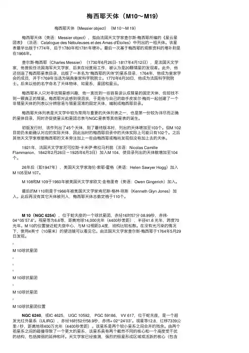
梅西耶天体(M10~M19)梅西耶天体(Messier object)(M 10~M 19)梅西耶天体(英语:Messier object),指由法国天⽂学家查尔斯·梅西耶所编的《星云星团表》(法语:Catalogue des Nébuleuses et des Amas d'Étoiles)中列出的⼀组天体。
该星表最早出版于1774年,后于1780年和1781年增补。
最后⼀次基于梅西耶的观察资料的增补则是在1966年。
查尔斯·梅西耶(Charles Messier)(1730年6⽉26⽇- 1817年4⽉12⽇),是法国天⽂学家,他曾担任法国海军天⽂学家,后来在经度局⼯作,被认为是20颗彗星的发现者。
此外,他还创造了梅西耶星表⽬录,出版了⼀本名为“梅西耶的天体”的星系⽬录,1764年,他成为皇家学会的成员,并于1769年当选为瑞典皇家科学院院⼠。
1770年6⽉30⽇,他成为法国科学院院⼠。
后来以他的名字命名了天体物体,如星系,星团和星云。
梅西耶本⼈只对寻找彗星感兴趣,他⼀直找到⼀些容易误认成彗星的固定天体,但却找不到⼀颗真正的彗星。
梅西耶对此感到很沮丧,于是他与⾃⼰的助⼿⽪埃尔·梅尚⼀起创建了⼀个⾮彗星天体的列表以分辨容易与彗星混淆的固定天体,编制成梅西耶⽬录。
梅西耶天体列表是天⽂学中较为常⽤与重要的天体列表之⼀,也是第⼀份较为详尽⽽正确的星体⽬录,同时亦促使星云和星团总表与NGC星表等其他星表的诞⽣。
初版发⾏时,该作列出了45个天体,到了最终版本时,列出的天体增加⾄103个。
但M 102⽬前仍未能确认对应的实际天体,因此当时的梅西耶⽬录中的天体实际上可能只有102个。
之后其他天⽂学家根据梅西耶的⽂本旁注加上⼀些由梅西耶或梅尚发现但没有加上去的天体。
1921年,法国天⽂学家尼可拉斯·卡⽶伊·弗拉马利翁(法语:Nicolas Camille Flammarion,1842年2⽉26⽇-1925年6⽉3⽇)加⼊M 104,使⽬录列出的天体数增加⾄104个。
跟cx330一样特殊的恒星,既没有恒星为邻,也缺少行星做伴,这颗诞生只有100万年的年轻恒星被美国航天局称为“宇宙中最孤独的恒星”。
美国航天局的钱德拉X射线天文望远镜于2009年首次发现了这一名为CX330的恒星,有关这一恒星的研究报告发表在最新一期英国《皇家天文学会月刊》上。
这颗孤独的恒星与1936年至1937年间爆发的恒星猎户座FU星类似,但CX330结构更紧凑、温度更高,也更巨大。
光年,长度单位,指光在真空中一年时间中行走的距离,即约九万四千六百亿公里。
更正式的定义为:在一儒略年的时间中(即365.25日,而每日相等于秒),在自由空间以及距离任何引力场或磁场无限远的地方,一光子所行走的距离。
因为真空中的光速是每秒299,792,458米(准确),所以一光年就等于9,460,730,472,580,800米。
(或5,786,101,150,000英里。
5,108,385,784,330,890海里或约等于9.46 × 10^15 m =9.46 拍米。
)(注:1千米(公里)=0.6214英里=0.540海里)光年一般是用来量度很大的距离,如太阳系跟另一恒星的距离。
光年不是时间的单位。
光由太阳到达地球需时约八分钟(即地球跟太阳的距离为八“光分”)。
已知距离太阳系最近的恒星为半人马座比邻星,它相距4.22光年。
我们所处的星系——银河系的直径约有七万光年。
假设有一近光速的宇宙船从银河系的一端到另一端,它将需要多于十万年的时间。
但这只是对于(相对于银河系)静止的观测者而言,船上的人员感受到的旅程实际只有数分钟。
这是由于特殊相对论中的移动时钟的时间膨胀现象。
目前天文观测范围已经扩展到200亿光年的广阔空间,它称为总星系。
与天文学中其它常用单位的换算:一秒差距等于3.26光年。
一光年等于63,240天文单位。
另外,光每秒大约行驶30万千米,每分钟行驶1800万千米,每小时行驶万千米,每天行驶万千米,每年行驶万千米。
arXiv:astro-ph/9902176v1 11 Feb 1999A&Amanuscriptno.(willbeinsertedbyhandlater)ASTRONOMY
ANDASTROPHYSICS
1.IntroductionTheHubbleSpaceTelescope(HST)allowsthederivationofcolormagnitudediagrams(CMDs)ofGalacticglobularclus-ters(GCs)whichextendtoalmostthefaintestvisiblestars,justabovethehydrogen-burninglimitforthenearestclusters(Kingetal.1998).TheseCMDscanbeusedtoextractluminosity2PiottoandZoccaliTable1.DataSet
M22HST30-9-1995F606W1100””F606W1200×3””F814W1100””F814W1200×3DUTCH15-4-1997V45””V1500””I45””I1500
M55HST4-11-1995F606W1100””F606W1200×5””F814W1100””F814W1200×5DUTCH15-4-1997V45””V1500””I45””I1500
M10HST10-10-1995F606W1100””F606W1200×9””F814W1100””F814W1200×9JKT30-5-1997V15””V45””V1500””I15””I45””I1500HSTLFsofM10,M22,andM553magnitudeswasperformedbycomparisonwiththestarsintheoverlappingHSTfields.Wefirstadoptedthecolortermob-tainedforthesametelescopesduringthepreviousnightsinthesamerun(Rosenbergetal.1999).Thezeropointshavebeencalculatedbycomparingallthenon-saturatedstarsintheWFPC2chipsthatwerealsomeasuredintheground-basedim-ages.TheuncertaintiesintheVzeropointsare0.004,0.035,and0.015magnitudes(theerrorsrefertotheerrorsonthemeandifferences)forM10,M22,andM55,respectively.Theerrorsinthe(V−I)colorsare0.006,0.055,and0.025,re-spectively.ThezeropointuncertaintiesforM22arenoticeablylargerthanfortheothertwoclusters.Thisfactisduetothesmalleroverlapinmagnitudebetweentheground-basedandtheHSTphotometries,ascanbeseeninFig.2.Thecalibra-tionoftheM22andM55CMDshasbeenfurthercheckedbycomparingthesediagramswithotherindependentlycalibratedVvs.(V−I)ground-basedCMDskindlyprovidedbyAlfredRosenberg(Rosenbergetal.1999).Thetwosetsofdataareconsistentwithintheuncertaintiesgivenabove.Shorter-exposureHSTimages(orlonger-exposureground-basedframes)aredesirableforasmootheroverlapofthetwodatasets.NotethatthisproblemdoesnotaffecttheLFpre-sentedinSection4.Indeed,azeropointerrorofafewhundredsofamagnitudeisperfectlyacceptableforaLFwithmagnitudebinsof0.5mag.
2.3.ArtificialstartestsParticularattentionwasdevotedtoestimatingthecomplete-nessofoursamples.Thecompletenesscorrectionshavebeendeterminedbystandardartificial-starexperimentsonboththeHSTandground-baseddata.Foreachcluster,weperformedtenindependentexperimentsfortheHSTimagesandfivefortheground-basedones.Inordertooptimizethecputime,inourexperimentswetriedtoaddthelargestpossiblenumberofartificialstarsinasingletest,withoutartificiallyincreasingthecrowdingoftheoriginalfield.TheartificialstarshavebeenaddedinaspatialgridsuchthattheseparationofthecentersineachstarpairwastwoPSFradiiplusonepixel.Thepositionofeachstarisfixedwithinthegrid.However,thegridwasran-domlymovedontheframeineachdifferentexperiment.Weverifiedthatinthiswaywewerenotcreatingover-crowdingbyrunninganexperimentwithhalfthenumberofartificialstars.Thefindingalgorithmadoptedtoidentifyandmeasurethearti-ficialstarswasthesameusedforthephotometryoftheoriginalimages.TheartificialstarswereaddedoneachsingleVandIframe.Foreachartificialstartest,theframetoframecoordinatetransformations(ascalculatedfromtheoriginalphotometry)havebeenusedtoensurethattheartificialstarswereaddedex-actlyinthesamepositionineachframe.WestartedbyaddingstarsinoneVframeatrandommagnitudes;thecorrespondingImagnitudeforeachstarwasobtainedusingthefiduciallineoftheinstrumentalCMD.Finally,ineachband,wescaledthemagnitudesaccordingtotheframetoframemagnitudeoffsetascalculatedfromtheoriginalphotometry.Theframesobtainedinthiswaywerestackedtogetherinordertoperformstarfind-Fig.1.CompositeCMDfor6986starsinM10.Theground-baseddataarefromtheJKTtelescope.ingandobtainthemostcompletestarlist.ThelatterwasusedtoreducethesingleframessimultaneouslywithALLFRAME,followingallthestepsandusingthesameparametersasontheoriginalimages.InordertotakeintoaccounttheeffectofthemigrationofstarstowardbrightermagnitudesintheLF(Stetson&Harris1988),wecorrectedforcompletenessusingthematrixmethoddescribedinDrukieretal.(1988).IntheLFspresentedhere,weincludeonlypointsforwhichthecompletenessfigureswere50%orhigher,sothatnoneofthecountshavebeencorrectedbymorethanafactorof2.Acomparisonbetweentheaddedmagnitudesandthemea-suredmagnitudesallowsalsoarealisticestimateofthepho-tometricerrorσpho(definedasthestandarddeviationofthedifferencesbetweenthemagnitudesaddedandthosefound)asafunctionofmagnitude.Weusethisinformationindifferentplacesinwhatfollows.3.Thecolor-magnitudediagramsTheCMDsderivedfromthephotometrydiscussedintheprevi-ousSectionarepresentedinFigs.1,2,and3.TheupperpartoftheCMDscomesfromtheground-baseddata,whilethelowerpartisfromthethreeWFcamerasoftheWFPC2.InthecaseofM22,theCMDformagnitudesfainterthanV=19.8comesfromtheWF2only:thedifferentialreddeningofthiscluster(Peter-sonandCudworth1994)makesthesequencemuchbroaderthanexpectedfromthephotometricerrors.TheMSofM22fromthethreeWFcamerasisshowninFig.4.InTable2the