LARGE SCALE PERTURBATIONS IN THE OPEN UNIVERSE

1.复杂（事物的种类、头绪等）多而杂。

——辞海In general usage, complexity tends to be used to characterize something with many parts in intricate arrangement. The study of these complex linkages is the main goal of complex systems theory.在通常的用法中，复杂往往用于描述具有错综排列的很多部件的物体。

研究这些复杂的联系是复杂系统理论的主要的目标。

——维基百科事物的种类、头绪等多而杂;具有各种不同的,而且常是数量众多的部分、因素、概念、方面或影响是相互联系的,而这种相互联系又是难于分析、解答或理解。

——百度百科Neil Johnson describes complexity science as the study of the phenomena which emerge from a collection of interacting objects.[3]Neil Johnson将复杂科学描述成相互作用物体集合所产生现象的研究［3］。

从词源上，需要认识对象的数量过于巨大，和／或这些对象的性质存在差异且其组合关系又十分纠缠时，人们主观上形成一种缺乏统一性的不协调感，称为复杂。

复杂意指难于分割、分析或解决。

［4］2.复杂性在日常说法中，复杂或复杂性和简单相对立。

但在特定的场合，复杂的反面是各部分相互独立，而复杂化才与简单相对立。

日常生活中，“复杂（Complex）”经常与“复杂的（Complicated）”混用。

但在现今的系统科学中，它们一个是成千上万个相互连结着的“排烟管”，另一个则用来形容一些所谓高度“结合”在一起的解决方案。

(Lissack & Roos, 2000) 它是指，“复杂”（Complex）与“独立自主”相对的（译者注：在于突出系统各节点间错综复杂的联系），而“复杂的”（Complicated）才与“简单”相对（译者注：解决方案其内涵令人捉摸不清，让人产生一种复杂感，但是其结构却只是简单结合，并不复杂）。

小学上册英语第5单元期末试卷(含答案)英语试题一、综合题(本题有100小题，每小题1分，共100分.每小题不选、错误，均不给分)1.The goldfish has beautiful _______ (鳞片).2. A force acting in the opposite direction of motion is known as ______ (resistance).3.My sister enjoys __________ (做手工艺).4.The jellyfish floats in the _________ (海洋).5.The fish swims _____ (slowly/quickly) in the water.6. A saturated fat has no double ______.7. A _______ is a chart that organizes elements by their properties.8.What do you call the place where you learn about history?A. MuseumB. LibraryC. SchoolD. Park答案:A9.The __________ was an important period of change in the United States. (冷战)10.What is the name of the toy that you can build with blocks?A. PuzzleB. LegoC. DollD. Car答案: B11.The playground is _______ with children.12.The _____ (树木) provide shade on hot days.13.What is the name of the ocean that is the largest?A. Atlantic OceanB. Indian OceanC. Arctic OceanD. Pacific Ocean 答案: D14.I enjoy creating games with my toy ________ (玩具名称).15.Energy can be transformed from one form to _______.16.The cake is _____ (sweet/sour).17.My brother is a __________ (广告设计师).18.The chemical formula for palmitoleic acid is ______.19.What is the capital of the United States?A. New YorkB. Washington, D.C. C. ChicagoD. Los Angeles答案:B20.The tortoise carries its house on its _________. (背上)21.The process of evaporation causes liquids to turn into ______.22.The ______ contains a lot of water vapor.23.__________ are substances that can donate protons in a reaction.24.The ancient Romans built _______ to honor their leaders. (雕像)25.I _____ (love/hate) homework.26.The __________ (探险活动) is thrilling and educational.27.My favorite color is ________.28.The antelope runs very _________. (快)29.My toy ________ can zoom around the room.30.She is ________ (interested) in science.31.The stars are _____ (bright/dim) in the sky.32.The __________ is known for its stunning beaches.33.It is ___ (sunny) today.34. A rabbit's teeth never stop ______ (生长).35. A rabbit has powerful ______ (后腿) for jumping.36. A ______ (鸡) lays eggs every day.37.I _____ (want/wanted) to go to the park.38.What do you call a young goat?A. LambB. KidC. CalfD. Foal答案:B39.The hamster stores food in its ______ (脸颊).40. A solution is homogeneous, meaning it has a _______ composition.41.I like to help my mom ________ (整理) my room.42.Which fruit is known for having seeds on the outside?A. AppleB. StrawberryC. GrapeD. Pear答案:B.Strawberry43.I am proud of myself when I __________ because it shows __________.44.The process of photosynthesis occurs in the ______ (叶子).45.The __________ (希腊神话) includes many gods and heroes.46.We have math _____ today. (class/homework/friends)47. A dolphin can recognize itself in a ________________ (镜子).48.The __________ of an animal can vary greatly between species.49.The ________ has many petals and smells great.50.What is the color of the sky on a clear day?A. GreenB. BlueC. RedD. Yellow答案:B Blue51.The ______ is known for her photography.52.What is the first letter of the alphabet?A. BB. AC. CD. D答案:B53. A __________ is a mixture that can be separated by filtration.54.The ancient Egyptians used ________ for recording their history.55.The __________ is a large area of land used for agriculture. (农田)56.The ________ (生长周期) of a plant can vary.57. A ________ can swim in the ocean.58.The capital of the Maldives is ________ (马累).59.What is the capital of Ethiopia?A. Addis AbabaB. NairobiC. KampalaD. Khartoum答案:A. Addis Ababa60.Acids can donate ______ ions in solution.61.The _____ (猴子) loves to eat fruit.62.The snail carries its ______ (壳) on its back.63._____ (离子) in soil can affect plant health.64.The __________ (水域) is home to many fish.65.Water freezes at ______ degrees Celsius.66.My brother plays in a ____ (band) with his friends.67.The chemical symbol for bismuth is __________.68. A prism bends light to create a ______.69.Every year, we celebrate ________ (新年) with fireworks and family gatherings.70.I want to create a video game about my toy ____. (玩具名称)71.The _____ (大熊猫) is a rare animal that lives in China. 大熊猫是生活在中国的一种稀有动物。

briefings in functional genomics oxford -回复“Functional Genomics in Oxford: Unleashing the Potential of Genome Research”Introduction:Functional genomics is a rapidly evolving field of study that aims to understand the functions and interactions of genes in order to unravel the mysteries of life. The University of Oxford, with its esteemed reputation in scientific research, plays a pivotal role in advancing the frontiers of functional genomics. In this article, we will delve into the exciting world of functional genomics at Oxford, exploring the key focus areas, cutting-edge techniques, and significant contributions made by researchers in thisever-expanding field.1. Understanding Functional Genomics:Functional genomics encompasses the study of how the genome regulates biological processes and influences the phenotype of an organism. At Oxford, researchers employ various approaches, including computational biology, next-generation sequencing, andhigh-throughput screening, to enhance our understanding of gene function.2. Key Focus Areas at Oxford:a. Disease Research: Advances in functional genomics have paved the way for a deeper understanding of the genetic basis of diseases. Oxford researchers employ functional genomics techniques to unravel the complex mechanisms underlying diseases such as cancer, cardiovascular disorders, and neurodegenerative conditions, with the ultimate goal of developing targeted therapeutics.b. Epigenomics: The study of epigenetic modifications, such as DNA methylation and histone modifications, is a vibrant area of research at Oxford's functional genomics laboratories. By elucidating the role of epigenetics in gene expression and disease development, researchers are discovering novel therapeutic targets and potential biomarkers for early diagnosis.c. Gene Regulation: Oxford's functional genomics researchers investigate the intricate web of gene regulation mechanisms, including transcription factors, non-coding RNA, and chromatinstructure. The elucidation of these mechanisms enhances our knowledge of gene expression control, providing insights into normal development and disease progression.d. Functional Annotation of Genomes: Identifying the functions of genes encoded within a genome is a fundamental aim of functional genomics. Oxford researchers apply computational and experimental approaches to annotate gene functions, deciphering the roles of genes in various biological processes and shedding light on the evolutionary significance of gene function divergence.3. Cutting-Edge Techniques at Oxford:a. Next-Generation Sequencing (NGS): NGS technologies have revolutionized functional genomics research at Oxford. These high-throughput sequencing techniques allow for the characterization of entire genomes, transcriptomes, and epigenomes in a cost-effective and time-efficient manner. Researchers use NGS to unravel gene expression profiles, detect genetic variants, and investigate epigenetic alterations associated with diseases.b. CRISPR-Cas9 Genome Editing: Oxford researchers spearhead breakthroughs in CRISPR-Cas9-mediated genome editing, enabling precise manipulation of the genome to study gene function. This technique has expanded the possibilities of functional genomics research, offering unprecedented opportunities to elucidate the role of specific genes in disease mechanisms and therapeutic interventions.c. Functional Screens: High-throughput functional screens allow Oxford researchers to systematically identify genes involved in specific biological processes or diseases. These screens involve large-scale genetic perturbations, such as RNA interference (RNAi) or CRISPR knockout libraries, coupled with phenotypic analyses. By identifying genes essential for specific cellular functions, functional screens contribute to our understanding of gene function and potential therapeutic targets.4. Significant Contributions by Oxford Researchers:a. The Cancer Genome Atlas (TCGA): Oxford researchers were instrumental in the international collaboration that led to the creation of TCGA, a comprehensive catalog of genomic alterationsin various cancer types. TCGA has provided crucial insights into the genetic basis of cancer, paving the way for personalized medicine approaches and targeted therapies.b. ENCODE Project: As part of the ENCODE Project, Oxford researchers contributed to the functional annotation of the human genome. This project aimed to identify all functional elements within the genome, shedding light on gene regulation, non-coding RNA, and the three-dimensional architecture of the genome.c. Single-Cell Genomics: Oxford researchers have made significant contributions to the emerging field of single-cell genomics. By studying individual cells, researchers can unravel cellular heterogeneity, identify rare cell types, and investigate gene expression dynamics at unprecedented resolution. These insights have the potential to revolutionize our understanding of development, diseases, and therapeutic interventions.Conclusion:Functional genomics research at the University of Oxford continues to push the boundaries of our understanding of gene function andits impact on health and disease. Through their focused research areas, cutting-edge techniques, and noteworthy contributions, Oxford researchers play a crucial role in unraveling the mysteries of the genome. As the field of functional genomics continues to evolve, Oxford will undoubtedly remain at the forefront of groundbreaking discoveries with far-reaching implications for human health.。

1Popularity and Performance:A Large-Scale StudyPETER KRAFFT∗,JULIA ZHENG∗,and EREZ SHMUELI,Massachusetts Institute of TechnologyNICOL´AS DELLA PENNA,Australian National UniversityJOSHUA TENENBAUM and ALEX PENTLAND,Massachusetts Institute of Technology1.INTRODUCTIONSocial scientists have long sought to understand why certain people,items,or options become morepopular than others.One seemingly intuitive theory is that inherent value drives popularity.An alter-native theory claims that popularity is driven by the rich-get-richer effect of cumulative advantage—certain options become more popular not because they are higher quality but because they are alreadyrelatively popular.Realistically,it seems likely that popularity is driven by neither one of these forcesalone but rather both together.Recently researchers have begun using large-scale online experiments to study the effect of cumu-lative advantage in realistic scenarios[Salganik et al.2006],[Muchnik et al.2013],but there havebeen no large-scale studies of the combination of these two effects.We are interested in studying acase where decision-makers observe explicit signals of both the popularity and the quality of variousoptions.We derive a model for change in popularity as a function of past popularity and past perceivedquality.Our model implies that we should expect an interaction between these two forces—popularityshould amplify the effect of quality,so that the more popular an option is,the faster we expect it toincrease in popularity with better perceived quality.We use a data set from ,an online social investment platform,to support this hypothesis.2.MODELOur model describes the evolution of popularity of an individual action a(e.g.,choosing to buy a par-ticular brand or following a particular person).We assume afixed population of N agents that all havethe option to take action a at each of a series of discrete times.That is,at each time every agent decideswhether to take action a in that time step.We assume that agents want to make good choices,wherethe action being good is defined in some suitable domain-specific way.We also assume that at the end ofeach time step,all agents observe a single new signal of the action’s quality,as well as how many otheragents took the action in that step.We denote the number of agents taking the action at time t as n tand the signal of its quality at time t as q t.We assume agents attempt to evaluate whether the action isgood using Bayesian inference.In this case users are tasked with computing the posterior distributionP(good|q1,...,q t).Further we assume that agents choose whether to take the action at a particulartime step via probability matching,which means that each agent decides whether to take the actionat round t+1with probability P(good|q1,...,q t),i.e.agents match the probability that they take ac-tion a with the probability that the action is good.This assumption of probabilistic decision-makinghas precedent in cognitive science[Vul et al.2009],animal behavior[Prez-Escudero and de Polavieja2011],and economics[Anderson and Holt1997].∗Thefirst two authors contributed equally.Collective Intelligence2014.1:2•P.Krafft et al.Then,lettingαbe an arbitrary positive constant(used as a smoothing parameter),we haveP(good|q1,...,q t)=P(q t|good,q1,...,q t−1)P(q t|q1,...,q t−1)P(good|q1,...,q t−1)≈P(q t|good,q1,...,q t−1)P(q t|q1,...,q t−1)n t−1+αN+α,where the approximation follows from an interesting observation:Since users are probability match-ing,previous popularity actually approximates the posterior distribution from the last time step,and hence P(good|q1,...,q t−1)is given by the(smoothed)proportion of agents that chose to take the action in the last time step.Finally,noting that by the same argument future popularity will estimate P(good|q1,...,q t),assum-ingαis small relative to N,and letting f(q1,...,q t)=P(q t|good,q1,...,q t−1)P(q t|q1,...,q t−1),we see that the expected change in popularity in the next time step is given byn t+1−n t≈(f(q1,...,q t)−1)·n t+f(q1,...,q t)·α.When f is a monotonically increasing function of q t,this equation implies that we should expect a synergy between popularity and quality whereby increasing the popularity of an action should amplify the boost in popularity the action would get from a new signal of high quality.3.DATAThe data set we use to test this hypothesis was provided to us by the eToro company.eToro offers a website that incorporates several different trading platforms alongside a social trading network. Individuals can trade in the commodities,stock,and currencies markets.Furthermore,traders can conduct their own trades or view and copy trades made by other users,all using real money.The data set consists of transactions from June13,2011to November20,2013from their website,. One particularly interesting feature of the site is the ability that users have to mirror other users, automatically copying all of the trades they make.Importantly,users can choose who they want to mirror by viewing various measurements of performance as well as the current popularities of those traders.Thus the number of copiers a user has in the future,i.e.the future popularity of that user, could be influenced both by explicit signals of that user’s current popularity and of that user’s quality, indicated by eToro’s performance metrics.Although we do not have access to the signals that were actually displayed to the site’s users,we attempt to reconstruct proxies of these signals for our study.For popularity,we use a reconstructed version of the number of copiers each user has based on the transactions in our data.For quality,we use a rough measurement of recent performance:the performance of a user on a particular day is that user’s average expected daily return from closed trades in the last5business days(more specifically, the average over the subset of those days on which a user had any trading activity).In this work,we use100consecutive days of data,(ranging from September09,2011until December 29,2011rather than thefirst100to ensure we have good estimates of popularity),and we reserve the remainder of the data for validation in a planned extension of the current study.This subset includes the trading activity of24,587users.4.RESULTSTo support our model and our hypothesis,we approximate f by a linear function of performance.Our hypothesis then reduces to showing that there is a positive significant interaction between past popu-larity and past performance in a linear regression of change in popularity for each user.To investigate this interaction,we use our measurements of the popularity and performance of each user on each day. The regressions we examine include data points that consist of the performance of each active user on each day,the popularities of those users on those days,and the popularities of those users on the Collective Intelligence2014.Popularity and Quality:A Large-Scale Study•1:30.000.040.080.12Low Popularity ConditionBinned Past Performance M e a n D i f f e r e n c e i n P o p u l a r i t y <=−50−25025>=50Popularity 0Popularity 112345−40−2002040Average Change in Popularity (Middle Popularity Condition)Binned Past PopularityB i n n e d P a s t P e r f o r m a n ce 0.00.51.01.52.02.5Fig.1.Left:Plot of mean change in popularity against performance (for user-day pairs with popularity zero or one and with 95%confidence Gaussian error bars on the means and regression lines fitted from raw data).To visualize the results of the regression better,we rounded performance to the nearest multiple of 25and grouped values greater than 50or less than −50with those numbers,respectively .These graphical parameters roughly balanced the bin sizes on the x-axis.The difference in slope between the two lines in the third plot displays the hypothesized interaction effect.Right:Heat map of mean change in popularity as a function of previous popularity and previous performance for users with greater than zero copiers not in the top 100most-popular group.For this plot we binned popularities greater than 5with 5,and we rounded performance to the nearest 10and grouped values less than −40or greater than 40with those numbers,respectively .The nonlinear increase in the third dimensions moving up and to the right in this plot displays the hypothesized interaction.following days.For the present analysis,we look only at the subset of day-user pairs on which the user did not lose followers.We make this restriction because once a user has more copiers,it is naturally easier for that user to lose copiers,and this effect could alone give the interaction we hope to provide evidence for.Since we are also interested in replicating the widely observed cumulative advantage marginal effect of past popularity on future popularity ,we also attempt to control for a position bias in the interface of the eToro website.Since users can rank traders by eToro’s measurements of performance or by popularity ,traders might gain followers just by being displayed prominently on the website.A position bias should not artificially introduce an interaction since users can only sort by one signal at a time,but it could induce artificial marginal effects.To do this control,we further subset the data into two groups:user-day pairs on which the user had 0or 1past popularity (i.e.,zero copiers or one copier)and user-day pairs on which users had greater than 0past popularity but on which the user was not among the top 100most popular users.We use 100as the cutoff to be conservative.Since viewing the top 100traders requires scrolling several times,we would not expect the position bias to have an effect in either of these conditions.We attempt to provide evidence for our hypothesis within each of these conditions.Our hypothesized positive interaction effect and the marginal cumulative advantage effect of pop-ularity are supported in both conditions (p <10−5for all relevant regression coefficients).Figure 1displays our results.The plot on the left in Figure 1shows that having just one copier substantially increases the rate of increase in popularity as a function of performance over having no copiers.The plot on the right shows that a similar trend holds for greater values of popularity as well.We thus conclude that,for this range of popularity values,popularity may amplify the effect of performance in determining the magnitude of increase in future popularity .Perhaps the rich get richer for good reason.Collective Intelligence 2014.1:4•P.Krafft et al.AcknowledgementsThis research was partially sponsored by the Army Research Laboratory under Cooperative Agree-ment Number W911NF-09-2-0053.Views and conclusions in this document are those of the authors and should not be interpreted as representing the policies,either expressed or implied,of the sponsors. This material is based upon work supported by the National Science Foundation Graduate Research Fellowship under Grant No.1122374.Any opinion,findings,and conclusions or recommendations ex-pressed in this material are those of the authors(s)and do not necessarily reflect the views of the National Science Foundation.REFERENCESLisa R.Anderson and Charles rmation cascades in the laboratory.The American Economic Review(1997). Lev Muchnik,Sinan Aral,and Sean Taylor.2013.Social Influence Bias:A Randomized Experiment.Science(2013).Alfonso Prez-Escudero and Gonzalo G.de Polavieja.2011.Collective Animal Behavior from Bayesian Estimation and Probability Matching.PLoS Computational Biology(2011).Matthew J.Salganik,Peter Sheridan Dodds,and Duncan J.Watts.2006.Experimental Study of Inequality and Unpredictability in an Artificial Cultural Market.(2006).Edward Vul,Noah D.Goodman,Thomas L.Griffiths,and Joshua B.Tenenbaum.2009.One and done?Optimal decisions from very few samples.In Proceedings of the31st Annual Conference of the Cognitive Science Society.Collective Intelligence2014.。

高超声速飞行器自抗扰姿态控制器设计秦昌茂;齐乃明;朱凯【期刊名称】《系统工程与电子技术》【年(卷),期】2011(33)7【摘要】针对高超声速飞行器无动力再入过程中具有强耦合、气动参数摄动及不确定性的非线性姿态模型,结合自抗扰控制中的扩张状态观测器(extended state observer,ESO)及非线性状态误差反馈律(nonlinear law state error feedback,NLSEF),分别设计了高超声速飞行器内环和外环自抗扰姿态控制器.将不确定性、耦合及参数摄动等干扰作为"总和干扰"利用扩张状态观测器进行估计并动态反馈补偿,再利用NLSEF抑制补偿残差.自抗扰控制器(active disturbance rejection control,ADRC)设计无需精确的飞行器被控模型,也无需精确的气动参数及摄动界限.仿真结果表明,控制系统能够克服干扰及气动参数大范围摄动的影响,在获取良好的动态品质和跟踪性能的同时,具有较强的鲁棒性.%For the hypersonic vehicle nonlinear attitude mode in re-entry process unpowered with a strong coupling, aerodynamic parameter perturbations and non-deterministic, combining extended state observer ( ESO) and nonlinear law state error feedback ( NLSEF) in the active disturbance rejection cotrol ( ADRC) , the hypersonic vehicle inner and outer ADRC attitude controller are designed respectively. Interferences, such as uncertainty, coupling and parameter perturbations, are regarded as "the sum of interference" , the extended state observer is used to estimate and implement dynamic feedback compensation, and then the NLSEF is used to inhibit thecompensating residual. ADRC controller is designed without a precise model of vehicle, and without precise perturbation boundaries of aerodynamic parameters. Simulation results show that the control system can overcome the impact of large-scale perturbations of interference and aerodynamic parameters, which has good dynamic qualities, tracking capabilities, and strong robustness.【总页数】4页(P1607-1610)【作者】秦昌茂;齐乃明;朱凯【作者单位】哈尔滨工业大学航天工程系,黑龙江,哈尔滨,150001;哈尔滨工业大学航天工程系,黑龙江,哈尔滨,150001;哈尔滨工业大学航天工程系,黑龙江,哈尔滨,150001【正文语种】中文【中图分类】V448【相关文献】1.高超声速飞行器自抗扰分数阶PID控制器设计 [J], 秦昌茂;齐乃明;吕瑞;朱凯2.高超声速飞行器自抗扰PID姿态控制 [J], 齐乃明;宋志国;秦昌茂3.高超声速飞行器改进自抗扰串级解耦控制器设计 [J], 齐乃明;秦昌茂;宋志国4.高超声速飞行器再入姿态改进自抗扰控制 [J], 周啟航;野邵文;向政委;齐乃明5.高超声速飞行器的自抗扰控制器设计 [J], 闫斌斌;闫杰因版权原因，仅展示原文概要，查看原文内容请购买。

大爆炸后的重子声学振荡English response:The baryon acoustic oscillations (BAO) are fluctuations in the distribution of visible baryonic matter (normal matter) in the universe. These fluctuations are caused by acoustic density waves in the primordial plasma of the early universe. The BAO signal is imprinted in the large-scale structure of the universe and can be used as a standard ruler to measure the expansion history of the universe.After the Big Bang, the universe was filled with a hot, dense plasma of electrons, protons, and photons. Small perturbations in the density of this plasma created sound waves that propagated through the plasma. When the universe was about 380,000 years old and had cooled enough for the protons and electrons to combine and form neutral hydrogen atoms, the sound waves were frozen in place. These sound waves left a characteristic scale in the distribution ofmatter, known as the baryon acoustic oscillation scale.This scale can be observed in the large-scaledistribution of galaxies and used to measure the expansion history of the universe. By studying the BAO signal in the cosmic microwave background radiation and the distributionof galaxies, scientists have been able to constrain the parameters of the standard cosmological model and shedlight on the nature of dark energy.中文回答：重子声学振荡（BAO）是宇宙中可见重子物质（正常物质）分布的波动。

; br
astro-ph/9503004 1 Mar 95
OBSERVATIONAL CONSTRAINTS
At large scales we have to normalize the resulting power spectra by means of the COBE data. There are di erent approaches to this procedure. We are using the normalization proposed by Gorski et al.10 who calculated the multipole a9 of
Figure 1: The linear perturbation spectra of the BSI model (solid line), the standard CDM model (dashed line), and a model with a cosmological term (dashdotted line).
We have compared the theoretical predictions of di erent BSI spectra with such observational data as the variances calculated from the counts in cells, the angular correlation function, the Mach numbers, or the rms mass uctuations necessary for quasar and galaxy formation12 . These data appear to favour a spectrum with = 3 and an onset of extra power at about 2 h 1 Mpc. In that case the Hubble parameter is assumed to be 50 km/s/Mpc. On the other hand, recent observations with the HST suggest a big Hubble parameter of about 75 km/s/Mpc or even higher (see the contributions of W. Freedman and T. Shanks in these proceedings). Such a high Hubble parameter requires a nonzero cosmological term. This changes the predicted multipoles of the CMB uctuations. In Fig. 2 the multipoles for the Harrison-Zeldovich and BSI spectra in a CDM model with H = 50 km/s/Mpc are shown in comparison with a model with = 0:8, = 0:2, H = 75 km/s/Mpc.

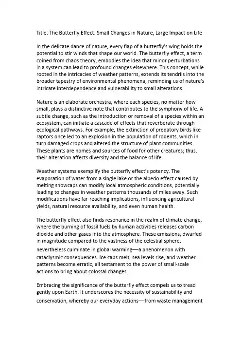
Title:The Butterfly Effect:Small Changes in Nature,Large Impact on LifeIn the delicate dance of nature,every flap of a butterfly's wing holds the potential to stir winds that shape our world.The butterfly effect,a term coined from chaos theory,embodies the idea that minor perturbations in a system can lead to profound changes elsewhere.This concept,while rooted in the intricacies of weather patterns,extends its tendrils into the broader tapestry of environmental phenomena,reminding us of nature's intricate interdependence and vulnerability to small alterations.Nature is an elaborate orchestra,where each species,no matter how small,plays a distinctive note that contributes to the symphony of life.A subtle change,such as the introduction or removal of a species within an ecosystem,can initiate a cascade of effects that reverberate through ecological pathways.For example,the extinction of predatory birds like raptors once led to an explosion in the population of rodents,which in turn damaged crops and altered the structure of plant communities. These plants are homes and sources of food for other creatures;thus, their alteration affects diversity and the balance of life.Weather systems exemplify the butterfly effect's potency.The evaporation of water from a single lake or the albedo effect caused by melting snowcaps can modify local atmospheric conditions,potentially leading to changes in weather patterns thousands of miles away.Such modifications have far-reaching implications,influencing agricultural yields,natural resource availability,and even human health.The butterfly effect also finds resonance in the realm of climate change, where the burning of fossil fuels by human activities releases carbon dioxide and other gases into the atmosphere.These emissions,dwarfed in magnitude compared to the vastness of the celestial sphere, nevertheless culminate in global warming—a phenomenon with cataclysmic consequences.Ice caps melt,sea levels rise,and weather patterns become erratic,all testament to the power of small-scale actions to bring about colossal changes.Embracing the significance of the butterfly effect compels us to tread gently upon Earth.It underscores the necessity of sustainability and conservation,whereby our everyday actions—from waste managementto energy consumption—are imbued with the understanding that they have far-reaching impacts.By choosing renewable energy sources,we can mitigate the ripple effect of fossil fuels on climate.By preserving ecosystems,we maintain the complexity of life that buffers against unforeseen changes.In conclusion,the butterfly effect is not merely a chaotic metaphor but a stark reminder of the interconnectedness of nature.Each creature,each action,and each decision we make is a thread in the vast web of life, influencing processes beyond our immediate perception.As we navigate the future,let this humbling insight guide our actions,fostering a deeper respect for the delicate balance that sustains us all.For indeed,in the realm of nature,every choice we make has the power to transform our world,just as the gentle flap of a butterfly's wings can herald the approach of a tempest.。

蝴蝶效应为话题英文作文600字全文共2篇示例，仅供读者参考蝴蝶效应为话题英文作文600字1:The butterfly effect, a concept originating from chaos theory, suggests that small changes can lead to significant outcomes in complex systems. In the context of your article, exploring this phenomenon provides a fascinating lens through which to analyze various aspects of life, ranging from the natural world to social dynamics and beyond.Introduction:The butterfly effect, coined by mathematician and meteorologist Edward Lorenz, illustrates the interconnectedness of events and the amplification of small perturbations over time. Although initially applied to weather forecasting, its implications extend far beyond meteorology.Theoretical Background:To delve deeper, it's essential to understand the mathematical underpinnings of chaos theory. At its core, chaos theory deals with systems that are highly sensitive toinitial conditions, meaning that small changes in the starting state can lead to vastly different outcomes. This sensitivity to initial conditions is exemplified by the butterfly effect.Application in Nature:In nature, the butterfly effect manifests in various ways. For instance, the flapping of a butterfly's wings in Brazil could set off a chain reaction of events that ultimately result in a tornado in Texas. This concept underscores the complexity and unpredictability of natural systems.Social Dynamics:Beyond the realm of nature, the butterfly effect is evident in social dynamics. A single action or decision by an individual can have ripple effects that reverberate throughout society. Whether it's a groundbreaking scientific discovery, a political revolution, or a viral social media post, seemingly small events can catalyze significant change.Real-World Examples:Numerous real-world examples illustrate the butterfly effect in action. Consider the case of Rosa Parks, whose refusalto give up her seat on a segregated bus sparked the Montgomery Bus Boycott and catalyzed the Civil Rights Movement. Similarly, the assassination of Archduke Franz Ferdinand of Austria set off a chain of events that led to World War I.Implications:Understanding the butterfly effect has profound implications for various fields, including economics, psychology, and even personal decision-making. It highlights the interconnectedness of systems and the need for humility in predicting outcomes. Moreover, it underscores the importance of considering the long-term consequences of our actions.Conclusion:In conclusion, the butterfly effect serves as a powerful metaphor for the interconnectedness and complexity of the world we inhabit. By embracing this concept, we gain insight into the underlying dynamics shaping our lives and the world at large. As you continue to explore this topic in your article, delve deeper into specific examples and implications toprovide a comprehensive understanding for your readers.蝴蝶效应为话题英文作文600字2:Title: The Butterfly Effect: Unraveling the Complexity of Small ActionsIntroduction:The concept of the butterfly effect, derived from chaos theory, suggests that small actions can have significant and unpredictable impacts on complex systems. It originates from the metaphorical idea that the flapping of a butterfly's wings in one part of the world could potentially cause a tornado in another part. This phenomenon underscores the interconnectedness and sensitivity of systems to initial conditions. Through exploring the butterfly effect, we gain insight into the intricacies of cause and effect relationships, highlighting the importance of understanding and managing complexity in various domains.Body:1. Origins and Development of the Butterfly Effect:The term "butterfly effect" was coined bymathematician and meteorologist Edward Lorenz in the 1960s while studying weather patterns. Lorenz's research revealed that small changes in initial conditions could lead to drastically different outcomes over time. This idea challenged traditional linear thinking and paved the way for the study of chaos theory.2. Examples of the Butterfly Effect in Nature:Nature provides numerous examples of the butterfly effect in action. For instance, the movement of a single bee pollinating flowers can have far-reaching effects on ecosystems by influencing plant reproduction and the food chain. Similarly, the introduction of a non-native species to an environment can disrupt the balance of an entire ecosystem, demonstrating how small actions can trigger cascading consequences.3. The Butterfly Effect in Human Systems:Beyond the natural world, the butterfly effect manifests in human systems as well. In economics, minor fluctuations in market conditions or consumer behavior can lead to significant fluctuations in stock prices or economic growth.Similarly, the spread of ideas and innovations can be traced back to small-scale actions that snowball into transformative societal changes.4. Applications and Implications:Recognizing the butterfly effect has practical applications in various fields. For instance, in risk management, understanding how small events can escalate into crises enables proactive measures to mitigate potential impacts. In decision-making processes, considering the long-term repercussions of seemingly insignificant choices can lead to more informed and strategic actions.5. Managing Complexity in a Butterfly Effect World:Living in a world characterized by the butterfly effect necessitates a paradigm shift in how we approach complexity. Embracing uncertainty and adopting systems thinking allows us to navigate interconnected networks with greater resilience and adaptability. By acknowledging our interconnectedness and the potential ripple effects of our actions, we can strive for more sustainable and equitable outcomes.Conclusion:The butterfly effect serves as a poignant reminder of the profound interconnectedness and unpredictability of the world around us. It challenges us to reevaluate our understanding of causality and complexity, urging us to consider the ripple effects of our actions on both natural and human systems. By embracing the lessons of the butterfly effect, we can cultivate a deeper appreciation for the power of small actions and the significance of interconnectedness in shaping our collective future.。

蝴蝶效应在现实生活中的意义英语作文Title: The Significance of the Butterfly Effect in Real LifeThe butterfly effect, a concept originating from chaos theory, illustrates the profound impact small initial changes can have on complex systems over time. In real life, this principle manifests in various aspects, shaping events and outcomes in unexpected ways.One significant realm where the butterfly effect is evident is in weather patterns. A seemingly minor alteration in atmospheric conditions, such as the flapping of abutterfly's wings, can potentially trigger a chain reaction leading to significant weather events elsewhere. This phenomenon underscores the interconnectedness of Earth's climate systems, emphasizing how seemingly insignificant actions can culminate in drastic consequences.Moreover, in social dynamics, small actions or decisions by individuals can catalyze large-scale societal shifts. For instance, a single act of kindness may inspire others to pay it forward, ultimately fostering a culture of compassion within a community. Conversely, a seemingly inconsequential choice, such as a careless remark, can escalate intoconflicts or misunderstandings with far-reaching ramifications.In economics, the butterfly effect is observable in market dynamics. A slight fluctuation in consumer behavior or investor sentiment can cascade through financial networks, influencing stock prices, consumer spending patterns, and overall market stability. This sensitivity to initial conditions underscores the unpredictability of economic systems and the importance of monitoring even the smallest perturbations.Furthermore, the butterfly effect resonates strongly in the realm of technology and innovation. A seemingly minor breakthrough in one field of science or technology cantrigger a cascade of innovations across multiple disciplines, leading to transformative advancements with wide-ranging implications for society. This interconnectedness underscores the collaborative nature of scientific progress and the importance of interdisciplinary research.On a personal level, the butterfly effect highlights the significance of individual agency and responsibility. Our everyday choices, no matter how seemingly inconsequential, contribute to shaping our own lives and the lives of those around us. Whether it be choosing to pursue a new hobby, cultivating healthy habits, or nurturing relationships, each decision sets off a chain of events that can profoundly impact our future trajectories.Moreover, the butterfly effect serves as a reminder of the interconnectedness of all living beings and ecosystems on Earth. A small change in one part of the world can have cascading effects on biodiversity, ecosystems, and theoverall health of the planet. This underscores the importance of environmental stewardship and collective action in addressing pressing global challenges such as climate change and habitat loss.In conclusion, the butterfly effect underscores the interconnectedness, complexity, and inherent unpredictability of the world we inhabit. From weather patterns to social dynamics, economics, technology, and personal choices, small initial changes can have profound and far-reaching consequences. Understanding and appreciating the significance of the butterfly effect empowers us to navigate complexity with mindfulness, responsibility, and a sense of interconnectedness with the world around us.。

2020年大学英语六级阅读理解试题及答案（卷五）Certainly no creature in the sea is odder than the common sea cucumber. All living creature，especially human beings，have their peculiarities，but everything about the little sea cucumber seems unusual. What else can be said about a bizarre animal that，among other eccentricities，eats mud，feeds almost continuously day and night but can live without eating for long periods，and can be poisonous but is considered supremely edible by gourmets?For some fifty million years，despite all its eccentricities，the sea cucumber has subsisted on its diet of mud. It is adaptable enough to live attached to rocks by its tube feet，under rocks in shallow water，or on the surface of mud flats. Common in cool water on both Atlantic and Pacific shores，it has the ability to suck up mud or sand and digest whatever nutrients are present.Sea cucumbers come in a variety of colors，ranging from black to reddish brown to sand color and nearly white. One form even has vivid purple tentacles. Usually the creatures are cucumber shaped-hence their name-and because they are typically rock inhabitants，this shape，combined with flexibility，enables them to squeeze into crevices where they are safe from predators and ocean currents.Although they have voracious appetites，eating day and night，sea cucumbers have the capacity to become quiescent and live at a lowmetabolic rate-feeding sparingly or not at all for long periods，so that the marine organisms that provide their food have a chance to multiply. If it were not for this faculty，they would devour all the food available in a short time and would probably starve themselves out of existence.But the most spectacular thing about the sea cucumber is the way it defends itself. Its major enemies are fish and crabs，when attacked，it squirts all its internal organs into water. It also casts off attached structures such as tentacles. The sea cucumber will eviscerate and regenerate itself if it is attacked or even touched; it will do the same if the surrounding water temperature is too high or if the water becomes too polluted.?1. According to the passage，why is the shape of sea cucumbers important??A. It helps them to digest their food.?B. It helps them to protect themselves from danger.?C. It makes it easier for them to move through the mud.?D. It makes them attractive to fish. ?2. The fourth paragraph of the passage primarily discusses______.?A. the reproduction of sea cucumbers?B. the food sources of sea cucumbers?C. the eating habits of sea cucumbers?D. threats to sea cucumbers' existence ?3. What can be inferred about the defence mechanisms of the sea cucumber??A. They are very sensitive to surrounding stimuli.?B. They are almost useless.?C. They require group cooperation.?D. They are similar to those of most sea creatures. ?4. Which of the following would NOT cause a sea cucumber to release its internal organs into the water??A. A touchB. Food?C. Unusually warm waterD. Pollution.【答案】1. B) 通过阅读文章可以排除选项A、C、D，因为文中没有提及，故选项B为正确答案。

1. Introduction
Now is the time to be a cosmologist. We have obtained through remarkable technological advances and heroic and ingenious experimental efforts a direct and extraordinarily detailed picture of the early Universe and maps of the distribution of matter on the largest scales in the Universe today. We have, moreover, an elegant and precisely quantitative physical model for the origin and evolution of the Universe. However, the model invokes new physics, beyond the standard model plus general relativity, not just once, but at least thrice: (1) Inflation, the physical mechanism for making the early Universe look precisely as it does, posits some new ultra-high-energy physics; we don’t know, however, what it is. (2) The growth of large-scale-structure and the dynamics of galaxies and galaxy clusters requires that we invoke the existence of collisionless particles or objects; we don’t know what this stuff is. (3) The accelerated expansion of the Universe requires the introduction of a new term, of embarrassingly small value, in Einstein’s equation, a modification of general relativity, and/or the introduction of some negative-pressure “dark energy,” again, the nature of which remains a mystery.

第一单元1.Condensed matter physics 凝聚态物理2.Atomic, molecular and optical physics 原子、分子、光学物理3.Particle and nuclear physics 粒子与原子核物理4.Astrophysics and physical cosmology 天体物理学和物理宇宙学5.Current research frontiers 当前研究前沿6.natural philosophy 哲学7.natural science 自然科学8.matter 物质9.motion 运动10.space and time 时空11.energy 能量12.force 力13.the universe 宇宙14.academic disciplines 学科15.astronomy 天文学16.chemistry 化学17.mathematics 数学18.biology 生物19.Scientific Revolution 科学革命20.interdisciplinary各学科间的21.biophysics 生物物理22.quantum chemistry 量子化学23.mechanism 机制24.avenues 渠道；大街25.advances 前进26.electromagnetism电磁学27.nuclear physics原子核物理28.domestic appliances家用电器29.nuclear weapons核武器30.thermodynamics热力学31.industrialization工业化32.mechanics力学33.calculus微积分34.the theory of classical mechanics经典力学35.the speed of light 光速36.remarkable卓越的37.chaos混沌38.quantum mechanics量子力学39.statistical mechanics 统计力学40.special relativity狭义相对论41.acoustics声学42.statics静力学43.at rest静止44.kinematics运动学45.causes原因46.dynamics动力学47.solid mechanics 固体力学48.fluid mechanics 流体力学49.continuum mechanics 连续介质力学50.hydrostatics流体静力学51.hydrodynamics流体动力学52.aerodynamics气体动力学53.pneumatics气体力学54.sound 声音55.ultrasonics超声学56.sound waves 声波57.frequency 频率58.bioacoustics生物声学59.electroacoustics电声学60.manipulation操作61.audible听得见的62.electronics电子63.visible light 可见光64.infrared红外线65.ultraviolet radiation 紫外线辐射66.reflection 反射67.refraction折射68.interference干涉69.diffraction衍射70.dispersion色散71.polarization偏振72.Heat 热度73.the internal energy内能74.Electricity 电力75.magnetism磁学76.electric current电流77.magnetic field磁场78.Electrostatics静电学79.electric charges电荷80.electrodynamics电动力学81.magnetostatics静磁学82.poles磁极83.matter and energy 物质和能量84.on the very large or very small scale 非常大或非常小的规模85.atomic and nuclear physics 原子与核物理学86.chemical elements化学元素87.The physics of elementary particles基本粒子88.high-energy physics 高能物理学89.particle accelerators 粒子加速器90.Quantum theory 量子论91.discrete离散92.subatomic原子内plementary互补94.The theory of relativity 相对论95.a frame of reference参考系96.the special theory of relativity 狭义相对论97.general theory of relativity 广义相对论98.gravitation万有引力99.universal law 普遍规律100.absolute time and space 绝对的时间和空间101.space-time 时空ponents组成103.Max Planck 普朗克104.quantum mechanics 量子力学105.probabilistic概率性106.quantum field theory量子场107.dynamical动态的108.curved弯曲的109.massive巨大的110.candidate候选111.quantum gravity 量子重力112.macroscopic宏观113.properties属性114.solids 固体115.liquids 液体116.electromagnetic force电磁力117.atom 原子118.superconducting超导119.conduction electrons 传导电子120.ferromagnetic 铁磁体121.the ferromagnetic and antiferromagnetic phases of spins铁磁和反铁磁的阶段的旋转122.atomic lattices原子晶格123.solid-state physics 固体物理124.subfields分区；子域125.nanotechnology纳米技术126.engineering工程学127.quantum treatments 量子治疗128.Atomic physics 原子物理129.electron shells电子壳层130.trap捕获131.ions离子132.collision碰撞133.nucleus原子核134.hyperfine splitting超精细分裂135.fission and fusion 分裂与融合136.Molecular physics 分子物理137.optical fields 光场138.realm范围139.properties属性140.distinct区别141.Particle physics 粒子物理142.elementary constituents基本成分143.interactions 相互作用144.detectors探测器puter programs程序146.Standard Model 标准模型147.quarks and leptons轻子-夸克148.gauge bosons规范波色子149.gluons胶子150.photons光子151.nuclear power generation核发电152.nuclear weaponsh核武器153.nuclear medicine 核医学154.magnetic resonance imaging磁共振成像155.ion implantation离子注入156.materials engineering 材料工程157.radiocarbon dating放射性碳测定年代158.geology 地质学159.archaeology考古学.160.Astrophysics天体物理学161.astronomy天文学162.stellar structure恒星结构163.stellar evolution恒星演化164.solar system太阳系165.cosmology宇宙学166.disciplines学科167.emitted射出168.celestial bodies天体169.Perturbations扰动170.interference干扰171.Physical cosmology 宇宙物理学172.Hubble diagram哈勃图173.steady state 定态，稳恒态174.Big Bang nucleo-synthesis核合成175.cosmic microwave background宇宙微波背景176.cosmological principle 宇宙论原理；宇宙论原则177.cosmic inflation宇宙膨胀178.dark energy 暗能量179.dark matter暗物质of high-temperature superconductivity 高温超导180.spintronics自旋电子学181.quantum computers 量子电脑182.the Standard Model 标准模型183.neutrinos中微子184.solar太阳185.the TeV万亿电子伏186.the super-symmetric particles 超对称粒子187.quantum gravity 量子重力188.superstring超弦189.theory and loop圈190.ultra-high energy cosmic rays高能宇宙射线,191.the baryon asymmetry重子不对称,192.the acceleration of the universe and the anomalous宇宙的加速和异常193.rotation旋转194.galaxies星系.195.turbulence动荡196.water droplets 水滴197.mechanisms of surface tension catastrophes表面紧张灾难198.heterogeneous多相的199.aerodynamics 气体力学第二单元所有的红色单词，重要的我标有星号1.classical mechanics 经典力学*2.physical laws 物理定律3.forces 力4.macroscopic 宏观的5.Projectiles 抛射体6.Spacecraft 太空飞船7.Planets 行星8.Stars 恒星9.Galaxies 星系,银河系10.gases, liquids, solids 气体,液体固体11.the speed of light 光速12.quantum mechanics 量子力学*13.the atomic nature of matter 物质的原子性质14.wave–particle duality 波粒二象性*15.special relativity 狭义相对论*16.General relativity 广义相对论*17.Newton's law of universal gravitation 牛顿万有引力*18.Newtonian mechanics 牛顿力学*grangian mechanics 拉格朗日力学*20.Hamiltonian mechanics 哈密顿力学*21.analytical mechanics 分析力学*22.as point particles 质点*23.Negligible 微不足道的可忽略的24.position, mass 位置,质量25.Forces 力26.non-zero size 不计形状27.the electron 电子*28.quantum mechanics 量子力学*29.degrees of freedom 自由度*30.Spin 旋转posite 组合的32.center of mass 质心33.the principle of locality 局部性原理34.Position 位置35.reference point 参照点(参照物)*36.in space 在空间37.Origin 原点*38.the vector 矢量39.Particle 质点*40.Function 函数41.Galilean relativity 伽利略相对性原理*42.Absolute 绝对43.time interval 时间间隔44.Euclidean geometry 欧几里得几何学45.Velocity 速度46.rate of change 变化率47.Derivative 倒数*48.Vector 矢量49.Speed 速度50.Acceleration 加速度*51.second derivative 二阶导*52.Magnitude 大小(量级)53.the direction 方向54.or both55.Deceleration 加速度56.Observer 观察者57.reference frames 参考系*58.inertial frames 惯性系*59.at rest60.in a state of uniform motion 运动状态一致61.Straight 直的62.physical laws 物理学定理63.non-inertial 非惯性系64.accelerating 加速65.fictitious forces 虚拟力(达朗贝尔力)*66.equations of motion 运动学方程*67.the distant stars 遥远的恒星68.Newton 牛顿69.force and momentum 力和动量70.Newton's second law of motion 牛顿第二定律*71.(canonical) momentum 动量* force 净力73.ordinary differential equation 常微分方程*74.the equation of motion 运动学方程*75.gravitational force 重力*76.Lorentz force 洛伦兹力*77.Electromagnetism 电磁学*78.Newton's third law 牛顿第三定律*79.opposite reaction force 反作用力80.along the line 沿直线81.displacement 位移*82.work done 做功83.scalar product 标极*84.the line integral 线积分*85.path 路径86.conservative. 守恒*87.Gravity 重力88.Hooke's law 胡克定律*89.Friction 摩擦力*90.kinetic energy 动能*91.work–energy theorem 功能关系(动能定理)*92.the change in kinetic energy 动能改变量93.gradient 梯度*94.potential energy 势能*95.Conservative 保守的,守恒的96.potential energy 势能97.total energy 总能量(机械能)*98.conservation of energy 能量守恒**99.linear momentum 线动量100.translational momentum 平移动量101.closed system 封闭系统*102.external forces 外力*103.total linear momentum 总(线)动量线动量就是动量区别于角动量104.center of mass 质心*105.Euler's first law 欧拉第一定律106.elastic collision 弹性碰撞*107.inelastic collision 非弹性碰撞*108.slingshot maneuver 弹弓机动109.Rigidity 硬度(刚性)*110.Dissipation 损耗**111.inelastic collision 非弹性碰撞112.heat or sound 热或声113.new particles 新粒子114.angular momentum 角动量*115.moment of momentum 瞬时动量*116.rotational inertia 转动惯量*117.rotational velocity 转速*118.rigid body 刚体**119.moment of inertia 惯性力矩*120.angular velocity 角速度*121.linear momentum 线动量122.Crossed 叉乘*123.Position 位置124.angular momentum 角动量125.pseudo-vector 赝矢量*126.right-hand rule 右手规则 external torque 净外力转矩128.neutron stars 中子星129.angular momentum 角动量*130.Conservation 守恒131.Gyrocompass 陀螺罗盘132.no external torque 无外力炬133.Isotropy 各向同性*134.Torque 转矩135.central force motion 中心力移动136.white dwarfs, neutron stars and black holes 白矮星,中子星,黑洞第三单元ThermodynamicsThermodynamics: 热力学；热力的Heat ：热；热力；热度Work：功macroscopic variables：肉眼可见的；宏观的，粗观的，粗显的。

小学下册英语第五单元测验卷(有答案)考试时间：80分钟（总分:100）A卷考试人：_________题号一二三四五总分得分一、综合题(共计100题共100分)1. 填空题：The __________ (历史的研究) uncovers hidden narratives.2. 选择题：Which color is a stop sign?A. BlueB. YellowC. RedD. Green3. 选择题：Which type of tree produces acorns?A. PineB. MapleC. OakD. Birch答案:C4. 听力题：We are going ________ a trip.5. 填空题：The __________ is a large expanse of tundra in the Arctic. (冻土)6. 填空题：I can ______ (分析) my progress and set new goals.7. 填空题：My friend is a __________ (探险家).8. 听力题：Astrobiology studies the possibility of ______ in the universe.9. 填空题：The tiger is a powerful _______ (捕食者).10. 选择题：What is the capital of Japan?A. TokyoB. BeijingC. SeoulD. Bangkok答案:A11. 选择题：What is the term for a group of words that expresses a complete thought?A. PhraseB. SentenceC. ClauseD. Paragraph答案: B12. 选择题：What is 3 x 4?A. 10B. 11C. 12D. 13答案: C. 1213. 选择题：What is the capital city of Italy?A. RomeB. FlorenceC. VeniceD. Milan答案:A14. 选择题：What do we call the large, wild cat that lives in Africa?A. LeopardB. TigerC. LionD. Cheetah答案: C15. 选择题：What is the term for the effect of gravity on time?A. Time DilationB. Gravitational TimeC. Temporal DistortionD. Space-Time Continuum16. 听力题：A ____ lives in water and has a smooth body.17. 听力题：Asteroids are mostly found in the ______ Belt.18. 听力题：The chemical symbol for chromium is _______.19. ts can survive in very ______ (极端) conditions. 填空题：Some pla20. 听力题：A chemical bond is formed when atoms ______.21. 选择题：What is the name of the famous river in France?A. SeineB. ThamesC. DanubeD. Rhine答案:A22. 选择题：What is the name of the famous mouse created by Walt Disney?A. Donald DuckB. GoofyC. Mickey MouseD. Pluto23. 听力题：My friend is very ________.24. 选择题：What do you call the force that pulls objects toward the Earth?a. Magnetismb. Gravityc. Frictiond. Pressure答案:B25. 填空题：The __________ is a famous city known for its museums. (巴黎)26. 填空题：The _____ (mint) plant grows quickly.27. 填空题：The ancient Egyptians used ________ to write their history.28. 听力填空题：I believe in the importance of empathy. Understanding how others feel helps us build strong connections. I practice empathy by __________ when talking to friends.29. 听力题：The children are _____ in the playground. (playing)30. 填空题：I love to watch ______ while I eat dinner.31. 填空题：A ______ (植物的生态研究) can yield important information.32. 填空题：The _____ (果树) is full of ripe fruit.33. 选择题：What is the name of the plant that grows in water and has broad leaves?A. CactusB. LilyC. FernD. Rose答案：B34. 填空题：The _______ (鱼) has colorful scales.35. 填空题：The __________ is the habitat for polar bears. (北极)36. 听力题：A _______ can be used for making dyes.37. 选择题：What is the capital of Iceland?A. ReykjavíkB. OsloD. Tallinn38. 听力题：I can ________ (adapt) to changes quickly.39. 选择题：What is 3 + 5?A. 7B. 8C. 9D. 1040. 选择题：What instrument do you blow to make music?A. PianoB. FluteC. DrumD. Violin41. 填空题：The ______ (植物的物种多样性) is crucial for resilience.42. 选择题：What do we call the area of land that is known for its unique climate and vegetation?A. BiomeB. EcosystemC. HabitatD. Region答案: A. Biome43. 填空题：A well-tended garden can be a source of fresh ______ all year round.(一个精心照料的花园可以全年提供新鲜的食材。

DOI: 10.1126/science.1224126, 366 (2012);338 Science et al.Yadong Sun Lethally Hot Temperatures During the Early Triassic GreenhouseThis copy is for your personal, non-commercial use only.clicking here.colleagues, clients, or customers by , you can order high-quality copies for your If you wish to distribute this article to othershere.following the guidelines can be obtained by Permission to republish or repurpose articles or portions of articles): October 18, 2012 (this information is current as of The following resources related to this article are available online at/content/338/6105/366.full.html version of this article at:including high-resolution figures, can be found in the online Updated information and services, /content/suppl/2012/10/17/338.6105.366.DC1.htmlcan be found at:Supporting Online Material /content/338/6105/366.full.html#related found at:can be related to this article A list of selected additional articles on the Science Web sites /content/338/6105/366.full.html#ref-list-1, 28 of which can be accessed free:cites 124 articles This article/content/338/6105/366.full.html#related-urls 1 articles hosted by HighWire Press; see:cited by This article has been registered trademark of AAAS.is a Science 2012 by the American Association for the Advancement of Science; all rights reserved. The title Copyright American Association for the Advancement of Science, 1200 New York Avenue NW, Washington, DC 20005. (print ISSN 0036-8075; online ISSN 1095-9203) is published weekly, except the last week in December, by the Science o n O c t o b e r 18, 2012w w w .s c i e n c e m a g .o r g D o w n l o a d e d f r o m10.L.Marrucci,C.Manzo,D.Paparo,Phys.Rev.Lett.96,163905(2006).11.G.Biener,A.Niv,V.Kleiner,E.Hasman,Opt.Lett.27,1875(2002).12.N.Yu et al .,Science 334,333(2011).13.M.Smit,J.van der Tol,M.Hill,Laser Photon.Rev.6,1(2012).14.C.R.Doerr,L.L.Buhl,Opt.Lett.36,1209(2011).15.K.J.Vahala,Nature 424,839(2003).16.Materials and methods are available as supplementarymaterials on Science Online.17.A.B.Matsko,A.A.Savchenkov,D.Strekalov,L.Maleki,Phys.Rev.Lett.95,143904(2005).18.D.Taillaert et al .,Jpn.J.Appl.Phys.45,6071(2006).19.R.Dorn,S.Quabis,G.Leuchs,Phys.Rev.Lett.91,233901(2003).20.Z.Bomzon,V.Kleiner,E.Hasman,Opt.Lett.26,1424(2001).21.A.Niv,G.Biener,V.Kleiner,E.Hasman,Opt.Express 14,4208(2006).22.I.Moreno,J.A.Davis,I.Ruiz,D.M.Cottrell,Opt.Express18,7173(2010).23.A.Yariv,Electron.Lett.36,321(2000).24.Y.Yu,R.O ’Dowd,IEEE Photon.Technol.Lett.14,1397(1992).25.S.Manipatruni,Q.Xu,M.Lipson,Opt.Express 15,13035(2007).davac,D.Grier,Opt.Express 12,1144(2004).Acknowledgments:We thank M.Berry and M.Dennis(Department of Physics,University of Bristol,UK),S.Barnett (Department of Physics,University of Strathclyde,UK),and M.Padgett (Department of Physics,University of Glasgow,UK)for very useful discussions and C.Railton (Merchant Venturers School of Engineering,University of Bristol,UK)for providing the finite-difference time-domain simulation tool.J.W.is funded by European Union FP7FET-OPEN project PHORBITEC.Supplementary Materials/cgi/content/full/338/6105/363/DC1Materials and Methods Supplementary Text Figs.S1to S7References (27–31)Movies S1to S425June 2012;accepted 10September 201210.1126/science.1226528Lethally Hot Temperatures During the Early Triassic GreenhouseYadong Sun,1,2*Michael M.Joachimski,3Paul B.Wignall,2Chunbo Yan,1Yanlong Chen,4Haishui Jiang,1Lina Wang,1Xulong Lai 1Global warming is widely regarded to have played a contributing role in numerous past biotic crises.Here,we show that the end-Permian mass extinction coincided with a rapid temperature rise to exceptionally high values in the Early Triassic that were inimical to life in equatorial latitudes and suppressed ecosystem recovery.This was manifested in the loss of calcareous algae,the near-absence of fish in equatorial Tethys,and the dominance of small taxa of invertebrates during the thermal maxima.High temperatures drove most Early Triassic plants and animals out of equatorial terrestrial ecosystems and probably were a major cause of the end-Smithian crisis.Anthropogenic global warming likely is contributing to the rapid loss of biolog-ical diversity currently occurring (1).Cli-mate warming also has been implicated in severe biotic crises in the geological past,but only as a corollary to more direct causes of death such asthe spread of marine anoxia (2).Here,we show that lethally hot temperatures exerted a direct control on extinction and recovery during and in the aftermath of the end-Permian mass ex-tinction.As well as the scale of the losses,the aftermath of this event is remarkable for severalreasons,such as the prolonged delay in recov-ery (3),the prevalence of small taxa (4),and the absence of coal deposits throughout the Early Triassic (5).These and several facets of low-latitude fossil records shown below,including fish,marine reptile,and tetrapod distributions,can be related to extreme temperatures in excess of tolerable thermal thresholds.Climate warming long has been implicated as one cause of the end-Permian crisis (2,6),with carbon dioxide release from Siberian eruptions and related processes providing a potential trig-ger for it (7,8).Conodont apatite oxygen isotope1State Key Laboratory of Geobiology and Environmental Geology,China University of Geosciences (Wuhan),Wuhan 430074,People ’s Republic of China.2School of Earth and En-vironment,University of Leeds,Leeds LS29JT,UK.3GeoZentrum Nordbayern,Universität Erlangen-Nürnberg,Schlossgarten 5,91054Erlangen,Germany.4Institute of Earth Sciences –Geology and Paleontology,University of Graz,Heinrichstrasse 26,A-8010Graz,Austria.*To whom correspondence should be addressed.E-mail:eeys@Fig.1.Early Triassic pa-leogeography showing reported occurrences of fish and marine reptiles in the Smithian.Note rare equatorial occurrence of both groups when ich-thyosaurs had evolved in northern climes.The global distribution of tetrapods (25)indicates occurrences almost ex-clusively in higher lati-tudes (>30°N and >40°S)throughout the Early Tri-assic,with rare exceptions in Utah (Parotosuchus sp.,paleolatitude ~10°N)and Poland (paleolatitude ~20°N),both probably of middle-late Spathian age (25,26).(Inset )Paleo-geography of Pangea and Nanpanjiang Basin after (45–47).Fish and ichthyo-saurs occurrences,see table S2.GBG,Great Bank ofGuizhou.19OCTOBER 2012VOL 338SCIENCE 366REPORTSo n O c t o b e r 18, 2012w w w .s c i e n c e m a g .o r g D o w n l o a d e d f r o mFig.2.Oxygen isotopes of conodont apatite and carbon isotopes of carbonates from the Nanpanjiang Basin.Oxygen isotopes show two thermal maxima in the late Griesbachian and late Smithian.Scanning electron microscope investigation of conodont surfaces shows microreticulation and no sign of recrystallization (supple-mentary text 3).Absolute age constraints are given in supplementary text 9;data for Meishan and Shangsi sections compiled from (9);leaf icons represent marine and terrestrial C 3plants (14).Modern equatorial SST ranges (annual mean)from (48).The error bar stands for external reproducibility of d 18O apatite measurements (2s ).The black trendline represents smoothed d 18O apatite fluctuations estimated from the upper water column taxa.Note uncertainty of correlating conodont zones with ab-solute ages.Aeg.,Aegean;Bith.,Bithynian.Conodont zonations:1,Ng.changxingensis ;2,Ng.yini ;3,Ng .meishanensis ;4,H.changxingensis ;5,H.parvus ;6,Is.staeschei ;7,Is.isarcica ;8,Ng.planata ;for genera abbreviations,see table S4.VSMOW,Vienna Standard Mean Ocean Water;VPDB,Vienna Pee Dee SCIENCEVOL 33819OCTOBER 2012367REPORTSo n O c t o b e r 18, 2012w w w .s c i e n c e m a g .o r g D o w n l o a d e d f r o mratio (d 18O)is a reliable proxy for paleoseawater temperatures (9),and conodonts suffered few genus-level losses at the end of the Permian (10),allowing continuous sampling of the same gen-era over multimillion-year intervals (11).We used d 18O apatite of conodonts from sections in the Nanpanjiang Basin,South China,to reconstruct Late Permian to Middle Triassic equatorial sea-water temperatures (Fig.1and supplementary text 1).Our main record,measured on the genus Neospathodus ,is a monitor of upper water col-umn temperatures (estimated ~70m water depth,supplementary text 2),whereas data from ex-tremely shallow water taxa (Pachycladina or Parachirognathus spp.,Platyvillosus spp.)pro-vide sea surface temperatures (SSTs).Our results show large,near-synchronous per-turbations in both carbon isotope ratios (d 13C carb )and d 18O apatite with three positive excursions observed in the Dienerian [~251.5million years ago (Ma)],early Spathian (~250.5Ma),and at the Spathian-Anisian (Early-Middle Triassic)transition (~247.5Ma).The minima in d 13C carb and d 18O apatite are measured in the Griesbachian (~252.1Ma)and the Smithian-Spathian transi-tion (~250.7Ma)(Fig.2).The d 18O apatite valuesof the analyzed conodonts taxa accord with their habitats in different water depth:Neospathodus spp.shows ~0.7per mil (‰)heavier values than those from shallow-water Pachycladina/Parachirognathus spp.and Platyvillosus spp.Deeper-water gondolellids show even heavier d 18O apatite (~0.4‰)than Neospathodus spp.(sup-plementary text 2and table S1).Latest Spathian –early Anisian oxygen isotope data from Bianyang and Guandao are more scattered and up to 1.3‰heavier compared with samples from other sec-tions.These two locations are close to the Great Bank of Guizhou (Fig.1),and such 18O enrich-ment toward platform interior is interpreted to be due to evaporation as seen on the modern Bahama Bank (12).However,most of the presented data are from distal,open-water environments and therefore present a faithful paleotemperature record (supplementary texts 3and 4).Calculation of seawater temperatures from d 18O values (supplementary text 5)reveals rapid warming across the Permian-Triassic boundary [21°to 36°C,over ~0.8million years (My);(9)],reaching a temperature maximum within the Griesbachian (~252.1Ma)followed by cooling in the Dienerian.A second rise to high temperaturesis seen in the late Smithian (~250.7Ma),followed by relatively stable temperatures in the Spathian,cooling at the end of this stage and stabilization in the early Middle Triassic (Fig.2).The late Smithian Thermal Maximum (LSTM)marks the hottest interval of entire Early Triassic,when up-per water column temperatures approached 38°C with SSTs possibly exceeding 40°C (Fig.3).The entire Early Triassic record shows tem-peratures consistently in excess of modern equa-torial annual SSTs.These results suggest that equatorial temperatures may have exceeded a tolerable threshold both in the oceans and on land.For C 3plants,photorespiration predom-inates over photosynthesis at temperatures in excess of 35°C (13),and few plants can survive temperatures persistently above 40°C (14).Sim-ilarly,for animals,temperatures in excess of 45°C cause protein damage that are only tem-porarily alleviated by heat-shock protein produc-tion (15).However,for most marine animals,the critical temperature is much lower,because metabolic oxygen demand increases with tem-perature while dissolved oxygen decreases (16).This causes hypoxaemia and the onset of an-aerobic mitochondrial metabolism that isonlyFig.3.Early Triassic diversity of major marine groups and temperature trends showing inverse relationship:Peak diversity corresponds to cool climate conditions around the Dienerian-Smithian boundary,early Spathian,and early Anisian (named cooling events I to III),whereas low diversity in Griesbachian and Smithian correlates with peak temperatures.Diversity of marine groups from (37–39,49–52);fish and marine reptile only show the general presence of taxa;no quantitative diversity data are available (sup-plementary text 6).Floral data (28–30,42)show the loss of equatorial conifer-dominated forests above the Permian-Triassic (PT)boundary,with the earlier reappearance of this forest type at high latitudes.Gray band represents the first-order seawater temperatures trend (upper water column,~70-m water depth)estimated by this study;red trend line represents possible SST derived from shallow water taxa.Same stratigraphic scheme as Fig.2.19OCTOBER 2012VOL 338SCIENCE368REPORTSo n O c t o b e r 18, 2012w w w .s c i e n c e m a g .o r g D o w n l o a d e d f r o msustainable for short periods (17).As a conse-quence,marine animals cannot long survive tem-peratures above 35°C,particularly those with a high performance and high oxygen demand,such as cephalopods (16).Extreme equatorial warmth should have left a distinct signature in the Early Triassic fossil records,a proposition that we examine here.The fossil fish record is exceptionally good in the Early Triassic,with many well-preserved faunas known from locations such as Madagas-car,Greenland,and British Columbia (supple-mentary text 6).This is related to the widespread distribution of anoxic facies (18)that provide ex-cellent preservational conditions for such fossils.However,our compilation of fish occurrences re-veals that they are very rare in equatorial locales,especially during the late Griesbachian and the Smithian,despite being common at higher lati-tudes at these times (fig.S1and table S2).This rarity is extraordinary because Early Triassic units,such as the dysoxic-anoxic Daye Forma-tion of South China,are widespread (supple-mentary text 7)and yet do not yield a fossil fish fauna.The general absence of ichthyofauna in equatorial regions coincides with the temperature maxima reconstructed from the d 18O apatite record,and we interpret this coincidence as recording equatorial exclusion because of inhospitably high temperatures.In contrast,invertebrates remain common in these intervals (19),especially sessile mollusks with their better adapted oxyconform-ing metabolism allowing them to cope with syn-ergistic stresses of high temperature and low oxygen (17,20).Like fish,marine reptiles also exhibit high aerobic activity and are likely to have had a relatively low oxygen-limited thermal tolerance.Examining Early Triassic marine rep-tile (ichthyosaur)occurrences reveals that they too are not found in equatorial waters until the middle-late Spathian (supplementary text 6),~1to 2My after their first appearance in higher latitudes during the Smithian (21,22).Other notable absences from equatorial oceans are cal-careous algae,whose outage spans the entire end-Permian –early Spathian interval although they are present in higher latitudes [e.g.,Spitsbergen,(23)].Their equatorial absence (supplementary text 8)likely reflects inhibiting temperatures,whereas the abundance of calcimicrobial carbon-ates in shelf waters,one of the stand-out features of the Early Triassic (24),was possible because of the much higher temperature tolerance of cyano-bacterial photosynthesis (16).Critically high temperatures may also have excluded terrestrial animal life from equatorial Pangea,and with SSTs approaching 40°C the land temperatures are likely to have fluctuated to even higher levels.Our compilation of tetra-pod fossil occurrences reveals them to be gen-erally absent between 30°N and 40°S in the Early Triassic (Fig.1),with rare exceptions (25,26);this is a stark contrast to Middle and Late Triassic occurrences,when they occur at all latitudes (fig.S1).This equatorial “tetrapod gap ”doesnot reflect an absence of suitable strata for their preservation.For example,the Buntsandstein of Europe is one of the best known and most in-tensively investigated terrestrial formations of the Early Triassic;tetrapods are exceptionally rare in the lower part (Induan)and only become common in middle and upper units (late Early Triassic to Middle Triassic)(27).The tetrapod gap of equatorial Pangea coincides with an end-Permian to Middle Triassic global “coal gap ”that indicates the loss of peat swamps (5).Peat for-mation,a product of high plant productivity,was only reestablished in the Anisian and then only in high southern latitudes (5),although gym-nosperm forests appeared earlier (in the Early Spathian),but again only in northern and south-ern higher latitudes (28,29).In equatorial Pangea,the establishment of conifer-dominated forests was not until the end of the Spathian (30),and the first coals at these latitudes did not appear until the Carnian ~15My after their end-Permian disappearance (5).These signals suggest equa-torial temperatures exceeded the thermal toler-ance for many marine vertebrates at least during two thermal maxima,whereas terrestrial equato-rial temperatures were sufficiently severe to sup-press plant and animal abundance during most of the Early Triassic.Thermal tolerance is likely to decrease for organisms with larger body sizes (31).Nonlethal effects of temperature increase include smaller adult size,which,in conjunction with increased juvenile mortality at higher temperatures (32,33),will produce a fossil record dominated by small individuals.This is a well-known phenomenon in the Early Triassic marine fossil record and has been termed the Lilliput effect (4).We suggest that this effect is a response to high tempera-tures and that it should be most clearly seen in equatorial assemblages,especially during the Griesbachian and Smithian thermal maxima.This prediction is confirmed by data from equatorial marine fossils where small body and trace fossil assemblages are confined to these intervals (34,35).Low oxygen levels also are known to cause small size in marine invertebrates (36),but,although marine dysoxia was a global phenomenon in the Early Triassic (18),the restriction of the Lilliput effect to equatorial latitudes indicates that this was primarily a temperature-controlled phenomenon.The relation between global warming and extinction can be examined in the Early Triassic.The rapid temperature rise across the Permian-Triassic boundary coincides with mass extinction,although absolute temperatures at the time of crisis were only modest [<30°C (9)].Together with temperature rise,synergistic factors,such as spread of anoxia,may also play important roles in marine extinction (2,18).However,the sub-sequent loss of many Permian holdover taxa later in the Griesbachian (conodonts,radiolarian,and brachiopods)may reflect lethal temperatures fol-lowed by temporary recovery and radiation in the cooler Dienerian (Fig.3).The clearest temperature-extinction link is with the LSTM and the end-Smithian event that saw major losses among many marine groups,including bivalves,cono-donts,and ammonoids (37–39).Contemporane-ous losses among tetrapods on land (25)suggest that this was a crisis that affected a broad di-versity of ecosystems.The ultimate driving factor behind the end-Permian warming long has been attributed to greenhouse gas emissions,either from volcano-genic (8)or thermogenic sources (40).Both are expected to leave a negative excursion in the d 13C record,and this is the case for both the end Permian –Griesbachian and Smithian intervals (Fig.2),although it has yet to be demonstrated that a second pulse of Siberian volcanism oc-curred in the Smithian.However,to maintain high temperatures for the ~5My of the Early Triassic requires strong,persistent greenhouse conditions.High temperatures also could greatly enhance the activity of decomposers (e.g.,fungi and bacteria),resulting in the release of large amounts of terrestrial light carbon into the at-mosphere (41)and consequently forming oligo-trophic,humus-poor soils as observed in modern Amazon rainforests and in Early Triassic soils of Australia and Antarctica (42).Together with global suspension of peat formation,elevated de-composition rates may have led to a significant reduction in organic carbon burial on land fur-ther contributing to higher atmospheric CO 2levels (43).High and oscillating temperatures in the Early Triassic likely controlled the pace and nature of recovery in the aftermath of the end-Permian mass extinction as shown by an inverse relation-ship between the temperature and biodiversity changes,the temporary loss of both marine and terrestrial vertebrates,and the reduced size of the remaining invertebrates.SSTs derived from d 18O data offer no evidence that a climate ther-mostat may ameliorate tropical warming by re-distributing warmth to the poles (44).Rather,extreme global warming may progressively force taxa to vacate the tropics and move to higher lat-itudes or become extinct.Marine organisms ex-hibiting low oxygen-dependent thermal tolerance,such as vertebrates,are the first to leave.References and Notes1.M.Bálint et al .,Nat.Clim.Change 1,313(2011).2.A.Hallam,P.B.Wignall,Mass Extinctions and Their Aftermath (Oxford Univ.Press,Oxford,1997).3.J.L.Payne et al .,Science 305,506(2004).4.R.J.Twitchett,Palaeogeogr.Palaeoclimatol.Palaeoecol.252,132(2007).5.G.J.Retallack,J.J.Veevers,R.Morante,Geol.Soc.Am.Bull.108,195(1996).6.D.L.Kidder,T.R.Worsley,Palaeogeogr.Palaeoclimatol.Palaeoecol.203,207(2004).7.M.K.Reichow et al .,Earth Planet.Sci.Lett.277,9(2009).8.S.V.Sobolev et al .,Nature 477,312(2011).9.M.M.Joachimski et al .,Geology 40,195(2012).10.D.L.Clark,W.Cheng-Yuan,C.J.Orth,J.S.Gilmore,Science 233,984(1986).rmation on materials and methods is available onScience Online.12.T.D.Frank,Data report:Geochemistry of Miocenesediments,Site 1006and 1007,Leeward margin,Great SCIENCEVOL 33819OCTOBER 2012369REPORTSo n O c t o b e r 18, 2012w w w .s c i e n c e m a g .o r g D o w n l o a d e d f r o mBahama Bank,in Proceedings of the Ocean Drilling Program,Scientific Results ,P.K.Swart,G.P.Eberli,M.J.Malone,J.F.Sarg,Eds.(Ocean Drilling Program,College Station,TX,2000),vol.166,pp.137–143.13.J.Berry,O.Bjorkman,Annu.Rev.Plant Physiol.31,491(1980).14.R.J.Ellis,Nature 463,164(2010).15.G.N.Somero,Annu.Rev.Physiol.57,43(1995).16.H.O.Pörtner,Comp.Biochem.Physiol.132,739(2002).17.H.O.Pörtner,Naturwissenschaften 88,137(2001).18.P.B.Wignall,R.J.Twitchett,Spec.Pap.Geol.Soc.Am.356,395(2002).19.T.Galfetti et al .,Sediment.Geol.204,36(2008).20.H.-O.Pörtner,J.Exp.Biol.213,881(2010).21.J.M.Callaway,D.B.Brinkman,Can.J.Earth Sci.26,1491(1989).22.C.B.Cox,D.G.Smith,Geol.Mag.110,405(1973).23.P.B.Wignall,R.Morante,R.Newton,Geol.Mag.135,47(1998).24.A.H.Knoll,R.K.Bambach,J.L.Payne,S.Pruss,W.W.Fischer,Earth Planet.Sci.Lett.256,295(2007).25.S.G.Lucas,Palaeogeogr.Palaeoclimatol.Palaeoecol.143,347(1998).26.M.Borsuk-Bia łynicka,E.Cook,S.E.Evans,T.Marya ń,Acta Palaeontol.Pol.44,167(1999).27.H.-D.Sues,N.C.Fraser,Triassic Life on Land (Columbia Univ.Press,New York,2010).28.T.Galfetti et al .,Geology 35,291(2007).29.E.Schneebeli-Hermann et al .,Palaeogeogr.Palaeoclimatol.Palaeoecol.339–341,12(2012).30.C.V.Looy,W.A.Brugman,D.L.Dilcher,H.Visscher,Proc.Natl.Acad.Sci.U.S.A.96,13857(1999).31.H.O.Pörtner,R.Knust,Science 315,95(2007).32.M.J.Angilletta,Thermal Adaptation-A Theoretical andEmpirical Synthesis (Oxford Univ.Press,New York,2009).33.J.A.Sheridan,D.Bickford,Nat.Clim.Change 1,401(2011).34.B.Metcalfe,R.J.Twitchett,N.Price-Lloyd,Palaeogeogr.Palaeoclimatol.Palaeoecol.308,171(2011).35.R.J.Twitchett,Palaeogeogr.Palaeoclimatol.Palaeoecol.154,27(1999).36.G.Chapelle,L.S.Peck,Nature 399,114(1999).37.S.M.Stanley,Proc.Natl.Acad.Sci.U.S.A.106,15264(2009).38.M.J.Orchard,Palaeogeogr.Palaeoclimatol.Palaeoecol.252,93(2007).39.J.Chen,in Mass Extinction and Recovery:Evidences fromthe Palaeozoic and Triassic of South China ,J.Rong,Z.Fang,Eds.(Univ.of Science and Technology of China Press,Heifei,2004),vol.II,pp.647–700.40.H.Svensen et al .,Earth Planet.Sci.Lett.277,490(2009).41.S.M.Stanley,Proc.Natl.Acad.Sci.U.S.A.107,19185(2010).42.G.J.Retallack,E.S.Krull,Aust.J.Earth Sci.46,785(1999).43.W.Broecker,S.Peacock,Global Biogeochem.Cycles 13,1167(1999).44.M.Huber,Science 321,353(2008).45.A.M.Ziegler,M.L.Hulver,D.B.Rowley,in Late Glacialand Postglacial Environmental Changes –Quaternary,Carboniferous-Permian and Proterozoic ,I.P.Martini,Ed.(Oxford Univ.Press,New York,1997),pp.111–146.46.G.Muttoni et al .,Geoarabia 14,17(2009).47.D.J.Lehrmann et al .,Palaios 18,138(2003).48.R.A.Locarnini et al .,World Ocean Atlas 2009,Volume 1:Temperature ,S.Levitus,Ed.[National Oceanic and Atmospheric Administration (NOAA)Atlas NESDros.Inf.Serv.68,ernment Printing Office,Washington,DC,2010].49.H.Song et al .,Geology 39,739(2011).50.D.Sun,S.Shen,in Mass Extinction and Recovery:Evidencesfrom the Palaeozoic and Triassic of South China ,J.Rong,Z.Fang,Eds.(Univ.of Science and Technology of China Press,Heifei,China,2004),vol.II,pp.543–570.51.H.Pan,D.H.Erwin,Palaeoworld 4,249(1994).52.L.O'Dogherty et al .,Geodiversitas 31,213(2009).Acknowledgments:D.Lutz,F.Nenning,B.Yang,and X.Liu are acknowledged for lab and field assistance.This study was supported by Chinese 973Program (2011CB808800)and the Natural Science Foundation of China (41172024and40830212).Y.S.acknowledges China University of Geosciences and China Scholarship Council for split-site Ph.D.at Wuhan,Leeds,and Erlangen.Supplementary Materials/cgi/content/full/338/6105/366/DC1Materials and Methods Supplementary Text Fig.S1Tables S1to S4References (53–150)1May 2012;accepted 4September 201210.1126/science.1224126A Complete Terrestrial Radiocarbon Record for 11.2to 52.8kyr B.P.Christopher Bronk Ramsey,1*Richard A.Staff,1Charlotte L.Bryant,2Fiona Brock,1Hiroyuki Kitagawa,3Johannes van der Plicht,4,5Gordon Schlolaut,6Michael H.Marshall,7Achim Brauer,6Henry mb,7Rebecca L.Payne,8Pavel E.Tarasov,9Tsuyoshi Haraguchi,10Katsuya Gotanda,11Hitoshi Yonenobu,12Yusuke Yokoyama,13Ryuji Tada,13Takeshi Nakagawa 8Radiocarbon (14C)provides a way to date material that contains carbon with an age up to ~50,000years and is also an important tracer of the global carbon cycle.However,the lack of a comprehensive record reflecting atmospheric 14C prior to 12.5thousand years before the present (kyr B.P.)has limited the application of radiocarbon dating of samples from the Last Glacial period.Here,we report 14C results from Lake Suigetsu,Japan (35°35′N,135°53′E),which provide a comprehensive record of terrestrial radiocarbon to the present limit of the 14C method.The time scale we present in this work allows direct comparison of Lake Suigetsu paleoclimatic data with other terrestrial climatic records and gives information on the connection between global atmospheric and regional marine radiocarbon levels.Lake Suigetsu contains annually laminated sediments that preserve both paleoclimate proxies and terrestrial plant macrofossils that are suitable for radiocarbon dating.The lake ’spotential to provide an important archive of at-mospheric radiocarbon (14C)was realized in 1993(1).However,the single SG93sediment core then recovered included missing intervals be-tween successive sections (2).This,together with the difficulty of visual varve counting,resulted in inconsistency between the SG93and other 14C calibration records (3).The SG06core-set re-covered in 2006consists of four parallel cores that together avoid any such sedimentary gaps (4).Here,we report 65114C measurements cov-ering the period between 11.2and 52.8thousand years before the present (kyr B.P .)tied to a time scale derived from varve counting and temporal constraints from other ing visual mark-ers,we applied a composite depth (CD)scale to all cores,including SG93.We also define an event-free depth (EFD),which is the CD with substan-tial macroscopic event layers (such as turbidites and tephras)removed.Accelerator mass spectrometry radiocarbon dating (5)has been conducted on terrestrial plant macrofossils selected from the SG06cores to cover the full 14C time range,from the present to the detection limit of the 14C method (0to 41m CD)(table S1).The results already reported from the control period (0to 12.2kyr B.P .)(6),covered by the tree-ring –derived calibration curve (7),act to demonstrate the integrity of the sediments and to anchor the floating SG06varve chronology,because varves do not extend into the Holocene.The varve-based chronology for SG06(5,8,9)provides our best estimate of the true age of the cores for the period ~10.2to 40.0kyr B.P .,based only on information from the site.It provides good relative chronological precision and has the advantage of being independent of other dating techniques.However,the cumulative counting un-certainty inevitably increases with age (~6%at 40kyr B.P .).The full varve chronology (Fig.1A and table S1)has been extrapolated on the basis of EFD to cover the period 40to 53kyr B.P .To better constrain the uncertainties in the varve chronology,we can directly compare the Suigetsu data set and other archives that provide information on atmospheric 14C and associated independent ages.The two most useful records for this purpose are the Bahamas speleothem GB89-25-3(10)and the Hulu Cave speleothem H82(11),both of which have extensive 14C-and U-Th –based chronologies.In both cases,we would ex-pect the radiocarbon in the speleothems to respond to changes in atmospheric 14C content,despite the groundwater containing a dead-carbon fraction (DCF)from dissolved carbonates.Estimated DCF for these speleothems was 2075T 270radiocarbon1University of Oxford,Oxford,UK.2Natural Environment Re-search Council Radiocarbon Facility,Scottish Universities Environmental Research Centre,East Kilbride,UK.3Nagoya University,Nagoya,Japan.4University of Groningen,Groningen,Netherlands.5University of Leiden,Leiden,Netherlands.6GeoForschungsZentrum German Research Centre for Geosci-ences,Potsdam,Germany.7Aberystwyth University,Aberystwyth,UK.8University of Newcastle,Newcastle upon Tyne,UK.9Free University Berlin,Berlin,Germany.10Osaka City University,Osaka,Japan.11Chiba University of Commerce,Chiba,Japan.12Naruto University of Education,Naruto,Japan.13University of Tokyo,Tokyo,Japan.*To whom correspondence should be addressed.E-mail:christopher.ramsey@19OCTOBER 2012VOL 338SCIENCE370REPORTSo n O c t o b e r 18, 2012w w w .s c i e n c e m a g .o r g D o w n l o a d e d f r o m。

关联波动英语Correlation FluctuationsThe concept of correlation fluctuations is a fundamental aspect of statistical physics and plays a crucial role in understanding the behavior of complex systems. In this essay, we will delve into the intricacies of correlation fluctuations, their significance, and their applications in various fields.Correlation is a statistical measure that quantifies the relationship between two or more variables. It describes the degree to which the variables are linearly related, with a value ranging from -1 to 1. When the variables are perfectly correlated, the correlation coefficient is either 1 (positive correlation) or -1 (negative correlation). In contrast, a correlation coefficient of 0 indicates that the variables are completely uncorrelated.Correlation fluctuations, on the other hand, refer to the variations in the correlation coefficient over time or across different realizations of a system. These fluctuations can arise due to various factors, such as the inherent randomness in the system, the finite size of the system, or the presence of external perturbations.One of the primary reasons why correlation fluctuations are important is their ability to reveal the underlying dynamics and interactions within a complex system. In many physical, biological, and social systems, the correlations between different variables are not constant but rather exhibit fluctuations over time or across different realizations. These fluctuations can provide valuable insights into the system's behavior, the nature of its interactions, and the mechanisms driving its evolution.For example, in the study of financial markets, correlation fluctuations between different asset prices can be used to identify patterns, detect market anomalies, and develop more effective trading strategies. In neuroscience, the study of correlation fluctuations in neural activity can shed light on the functional connectivity and information processing within the brain. In ecology, correlation fluctuations between different species populations can help researchers understand the complex dynamics of ecosystems and the impact of environmental changes.Furthermore, the study of correlation fluctuations has led to the development of powerful theoretical frameworks, such as the theory of critical phenomena and the theory of complex networks. These frameworks have enabled researchers to understand the universal behavior of systems near critical points, where small perturbationscan lead to large-scale changes, and to uncover the collective dynamics of interconnected systems.One of the key concepts in the study of correlation fluctuations is the notion of long-range correlations. In many complex systems, the correlations between different variables exhibit long-range or power-law decay, meaning that the correlations persist over large spatial or temporal scales. The presence of long-range correlations is often a signature of the system's complex and collective behavior, and it can have profound implications for the system's dynamics and response to external perturbations.The study of correlation fluctuations has also been instrumental in the development of new experimental and computational techniques. For instance, the use of advanced statistical methods, such as detrended fluctuation analysis and multifractal analysis, has enabled researchers to quantify and characterize the complex patterns of correlation fluctuations in a wide range of systems. Additionally, the increasing availability of large-scale data and the advancements in computational power have facilitated the analysis of correlation fluctuations in complex systems with unprecedented detail and precision.In conclusion, the study of correlation fluctuations is a vibrant and interdisciplinary field of research that has far-reaching implicationsfor our understanding of complex systems. By unraveling the intricate patterns of correlation fluctuations, researchers can gain valuable insights into the underlying dynamics and interactions that govern the behavior of physical, biological, and social systems. As the field continues to evolve, we can expect to see even more exciting discoveries and advancements that will deepen our understanding of the complex world around us.。

小学下册英语第六单元真题(含答案)考试时间：90分钟（总分:110）A卷一、综合题(共计100题共100分)1. 填空题：The ________ was a major event in the history of England.2. 填空题：My favorite fruit is _______ (西瓜).3. 听力题：The chemical formula for calcium phosphate is __________.4. 选择题：What do you call the time when the sun sets?A. DawnB. NoonC. DuskD. Midnight答案:C5. 填空题：The _____ (mint) plant grows quickly.6. 选择题：What do we call the place where we can see animals?A. ZooB. AquariumC. FarmD. Garden7. 填空题：The __________ is beautiful when covered with snow. (大地)8. 选择题：Which planet is known as the Red Planet?A. VenusB. EarthC. MarsD. Mercury答案: C9. 选择题：What do we call the part of the plant that absorbs water and nutrients from the soil?A. StemB. LeafC. RootD. Flower答案：C10. 填空题：I love to ______ (与他人分享) my insights.11. 填空题：Does your __________ (玩具名) have __________ (功能)?12. 选择题：What do we call the process of taking care of plants?A. GardeningB. FarmingC. HorticultureD. All of the above13. 填空题：I want to travel to ________ (不同国家) when I grow up. I want to see ________ (名胜古迹).14. 选择题：What is 100 divided by 4?A. 20B. 25C. 30D. 35答案:A. 2515. 填空题：The ______ (植物的生长方式) can differ significantly.16. 听力题：Sodium chloride is the chemical name for ______.When I travel, I like to take ______ (照片) to remember the places I’ve been. It’s nice to look back and see those memories.18. 选择题：What is the name of the first artificial satellite launched into space?A. VoyagerB. SputnikC. ApolloD. Challenger19. 听力题：The process of combining elements is called __________.20. 听力题：The capital of Serbia is __________.21. 填空题：The ______ (植物的适应性) is vital in changing climates.22. 选择题：What do you call the largest country in the world?A. CanadaB. United StatesC. RussiaD. China答案:C23. 听力题：A _______ is a reaction that occurs in the atmosphere.24. 听力题：The chemical formula for propane is __________.25. 选择题：What is the name of the imaginary line that goes around the Earth?A. EquatorB. LatitudeC. LongitudeD. Meridian答案:A26. 听力题：The ________ (puppet) is controlled by strings.Planting in groups can create a more dynamic and visually appealing ______. (成群种植可以创造出更具活力和视觉吸引力的景观。